New Evolutionary Algorithm for Optimizing Hydropower Generation Considering Multireservoir Systems

Abstract

In recent decades, solving complex real-life optimization problems has attracted the full attention of researchers. Dam and reservoir operation rules are considered one of the most complicated optimization engineering problems. In fact, the operation rules of dams and reservoirs are multisystematic and highly stochastic and have highly nonlinear system constraints due to the direct influence of environmental conditions: Therefore, these rules are considered highly complex optimization problems. Recently, metaheuristic methods inferred from nature have been broadly utilized to elucidate the way optimal solutions are provided for several complex optimization engineering applications, and these methods have achieved interesting results. The major advantage of these metaheuristic methods over conventional methods is the unnecessity to identify a particular initial condition, convexity, continuity, or differentiability. The present study investigated the potential of using a new metaheuristic method (i.e., the crow algorithm (CA)) to provide optimal operations for multireservoir systems, with the aim of optimally improving hydropower generation. A multireservoir system in China was considered to examine the performance of the proposed optimization algorithm for several operation scenarios. The results obtained the average hydropower generation by considering all examined operation scenarios based on the operation rule achieved using the CA, which outperformed the other metaheuristic methods. In addition, compared to other metaheuristic methods, the proposed CA lessened the time required to search for the optimal solution. In conclusion, the proposed CA has high potential for achieving optimal solutions to complex optimization problems associated with dam and reservoir operations.

1. Introduction

Increased population growth and industrial demands have caused an urgent need for not only the better planning of energy resources but also optimal generation rules [1]. Hydropower energy production is one of the real challenges for decision-makers and policymakers. Generated hydropower from hydropower plants attached to dams and reservoirs should be operated to supply the electrical hydropower required for population and industrial demands [2]. Electrical hydropower generation becomes a more vital problem when deficit events occur due to inappropriate operation rules: Thus, developing optimal operations for dams and reservoirs is essential [3].

One of the most important resources in the field of hydropower generation is that hydropower can be generated from water flow via hydropower plants attached to dams. A reservoir’s water storage upstream of the dam is operated based on different demands, such as irrigation and domestic, industrial, and environmental hydropower demands. Therefore, there is a need to develop operation rules for dam and reservoir systems to ensure the reliable production of hydropower generation. On the other hand, the upper bound of hydropower generation is limited to the full capacity of the hydropower plant. An operation rule that could achieve reliable and less probable risk to the hydropower generation pattern near full capacity is considered optimal [4].

Recently, researchers have applied several mathematical models to improve operation rules for the planning and management of hydropower production in dam and reservoir systems. The optimal generation of hydropower could be defined within the framework of an optimization problem [3]. Therefore, optimization algorithms, such as metaheuristic and evolutionary algorithms, could be used to search for the better operation of dam and reservoir systems to maximize the generation of hydropower. In fact, one or some objective functions are defined for these problems with the aim of increasing hydropower generation in hydropower plants based on released water from upstream dams [5]. Thus, released water from upstream dams is considered to be an unknown variable or decision variable, where the accurate determination of this variable has an effect on hydropower generation [6,7]. A real problem based on a multireservoir system with the aim of increasing hydropower generation is defined in this study with many complex constraints: This type of problem can be attractive for decision- and policymakers. This multireservoir system is in a chain sequence: In addition, three different scenarios are considered in this study to examine the proposed crow algorithm (CA) as an optimizer. The aim of the problem is maximizing hydropower generation based on the decision variable (i.e., reservoir capacity) during dry years (1963–1964), wet years (1951–1952), and normal years (1985–1986).

2. Review and Motivation

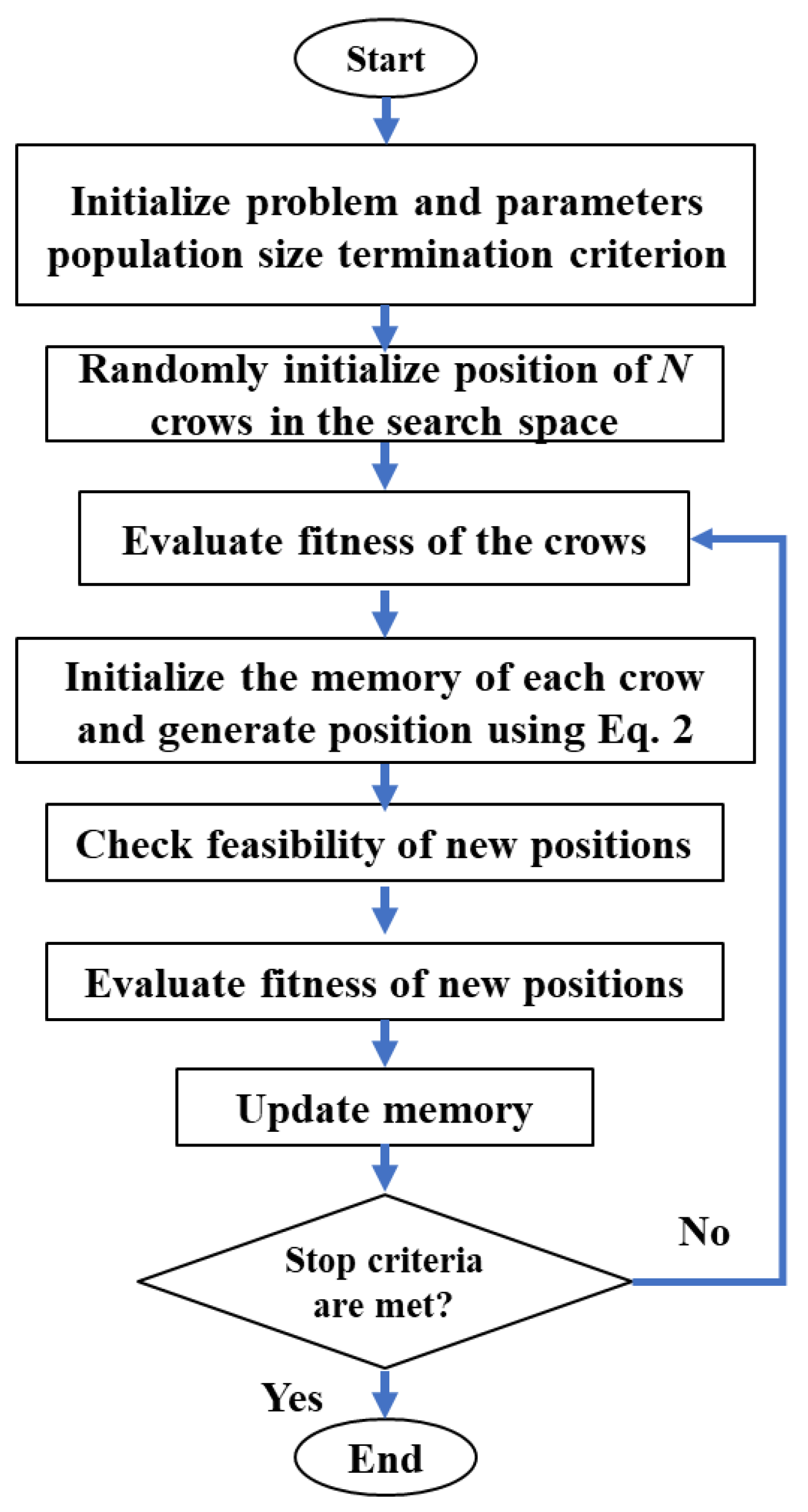
Hydropower production based on a multireservoir system is a complex problem when considering nonlinear objective functions and different constraints. Therefore, the extraction of an optimal solution and hydropower management based on released water from upstream dams are real challenges. Thus, solving such problems causes other researchers to try and understand different strategies for these complex problems. Several efforts have been developed to achieve optimal hydropower generation by utilizing different metaheuristic algorithms.

An optimization model has been developed to achieve reservoir operations with the aim of increasing hydropower generation while considering the environmental demand supply. The improved genetic algorithm (GA) was used for reservoir operations, and different flows in river regimes were considered for the optimization process. Nonlinear rule curves based on the GA were extracted for hydropower production, and the improved algorithm based on the elitism concept achieved more hydropower generation without trapping local optimal solutions [8,9,10]. Then, Arunkumar and Jothiprakash [11] used the improved particle swarm optimization (PSO) to increase hydropower production in multireservoir systems. The new PSO was generated based on the modification of acceleration coefficients in the PSO. The minimum required water amount for environmental demands was supplied, and the hydropower generated reached hydropower plant capacity based on the new PSO. In addition, an improved PSO was used for maximizing hydropower production and minimizing irrigation deficits at a large scale in China. The results indicated that the improved PSO based on the correction of the inertia coefficient had faster convergence over other versions of the PSO. Additionally, hydropower production based on an improved PSO reached hydropower plant capacity [12]. Furthermore, multireservoir operations based on a hybrid PSO and GA optimized performance with the aim of increasing hydropower production. The results indicated that the new hybrid algorithm could achieve more hydropower generation and faster convergence by covering the weak points of the GA and PSO based on increasing the diversity in the population [13,14].

The Bat algorithm has been used for increasing the annual benefit based on hydropower production in multireservoir systems and hydropower plants [15]. Released water was considered to be the decision variable, and the results indicated that the generated benefit based on hydropower production via the Bat algorithm had more value than the benefits via the GA and PSO. The Bat algorithm was performed based on the echolocation ability during a Bat’s life.

In recent years, Haddad et al. [16] have used the water cycle algorithm (WCA) for a 10-reservoir system, and the results indicated that the new algorithm decreased computation time with the inception of water-drop movement into the environment: Additionally, released water was considered to be the decision variable, and storage was considered to be the state decision. The position of water drops in rivers and seas was considered the decision variable for this algorithm. The biography-based optimization algorithm (BBA) has been used for the optimization of a four-reservoir system, and the aim of the problem was increasing the generated benefit based on generated hydropower [17]. Moreover, the firefly algorithm (FA) has been applied to multireservoir systems with the aim of increasing hydropower production [18]. In addition, the monarch butterfly (MBF) algorithm and krill algorithm (KA) have been applied for optimized hydropower generation based on the optimal operation rule for either single or multiple dam and reservoir systems [7,19].

The inception of swarm intelligence has caused algorithms to be directed toward the best solution to a problem with a minimum computation time. Problems with one or several objective functions can be simultaneously solved with such algorithms. For example, an increase in the reliability index, as a percent of the hydropower supply, and a decrease in the vulnerability index, as a percent of the shortage in hydropower production, can be simultaneously defined as two objective functions. These algorithms are highly adopted, which allows all effective variables influencing the system, such as hydraulic or hydrological constraints, to be defined within these algorithms. In other words, the algorithms can be adapted based on the system problem with a specific condition. The convergence procedure and global solution achieved within the optimization process are very important for the system under study. To some extent, the system is required to be operated in real-time: Therefore, a fast convergence rate is needed. In addition, when the system is highly nonlinear and stochastic in nature, a searching procedure for the optimal solution might be trapped in a suboptimal solution. Accordingly, there is a need to look for an optimization algorithm that could have the potential to encounter a high convergence rate and stochastic search procedure within its mathematical process. In addition, the algorithm should encounter advanced operators that could have a high chance of achieving a global solution within the searching domain.

In optimization theory, crows are the searchers: The environment can be considered the search space, and random storing positions can be taken as feasible solutions. The source that is best among all food sources is taken as the global solution, and the objective function is defined by the quality of the food source. By simulating the intelligence behavior of crows, the crow algorithm (CA) attempts to find the optimal solution to various optimization problems.

The novelty of the current research paper is not only the investigation of the potential of a new optimization algorithm, but also the application of the algorithm in a relatively complex reservoir system with multidimensional features for multireservoir systems under different climate condition scenarios. In fact, most of the previous research efforts have focused on the optimization algorithms’ performance, considering single reservoirs under single scenarios of climate change [10,11,12,13,14,15,16,17]: In addition, the evaluation of those optimization algorithms was basically based on common performance indices that might provide improper judgment on the real model performance. In fact, there are a few statistical indices that are usually used for evaluating the performance of optimization algorithms, such as reliability, resilience, and vulnerability. Reliability is the probability that the reservoir can supply the volume of water specified by the demand target in any given year. Resilience, on the other hand, is taken to be the conditional probability of experiencing a period of no failure (no water deficit) given that a failure occurred in the previous time period. The use of the resiliency measure allows the concept of resilience, which is the ability of the system to recover from a failure, to be more fully expressed. The final measure of performance is the vulnerability of the system. Vulnerability is the maximum deficit experienced in any one year. Meanwhile, in the current research, different indexes for comparing different algorithms have been proposed.

In this context, the present study attempts to investigate multireservoir performance under different climate conditions considering different reservoirs’ inflow scenarios (dry, wet, and normal conditions). Most of the existing research works have shown the superiority of the proposed optimization algorithms for single reservoir systems under a normal scenario only, which might be insufficient and inadequate for generalization to all cases of reservoir systems and under different scenarios of climate conditions.

3. Crow Algorithm

The CA, as a new evolutionary algorithm, is used in studies as a proposed optimization algorithm for dam and reservoir operations. Askarzadeh [20] has applied the CA to different benchmark functions and engineering optimization problems. The results indicated that the CA, based on two important parameters (flight length and awareness probability), could avoid trapping in the local solution, and the convergence rate was higher compared to those in other algorithms. Furthermore, Oliva et al. [21] applied the CA to an image processing application and achieved results that indicated that the CA outperformed other algorithms by obtaining a better image quality. However, the algorithm has some random parameters for which an accurate determination of these parameters is needed for accurate sensitivity, and the algorithm also has successful applications in the optimization of mathematical functions and structural engineering, but with some issues in power engineering.

The main advantage of the crow algorithm is that the updating mechanism employs a multidirectional search that advances and improves the diversity of solutions and can lead to avoiding being stuck in a local solution to enhance the possibility of achieving a global solution. This is often a prefect and optimal alternative among the available optimization algorithms in use, especially when dealing with more complex nonlinear and multimodal problems. The crow algorithm has been applied in several fields, such as civil engineering [22,23], medical science [24], and environmental science [25].

On the other hand, in the crow algorithm, a crucial influence on algorithm performance refers to the calculation of the hiding places of a crow. A basic implementation of this metaheuristic technique assumes a fixed value of the flight length that cannot be changed during iterations. As a result, the main drawback of this technique appears in the flight length value that the algorithm needs to cover the overall search space in finding the optimal solution. A small value of the flight length explores the solutions inside the line segment, and a large value of the flight length explores the solutions outside the line segment. Thus, this leads to using trial and error in assuming the initialization parameters.

Crows are known as being one of the largest bird species: Therefore, the ratio of their brain size to their body size is significant. The self-awareness of crows has been proven in different experiments [20]. Their powerful memories of different locations and faces is one of the most important characteristics of crows. Crows observe and follow other crows and birds to find their food and steal the food when given a good opportunity. The following assumptions are considered for crows:

• Flock life is considered for crows;
• Crows use powerful memories to recall hidden food by other birds or crows;
• Crows follow each other to steal hidden food;
• Crows hide their food based on their awareness of the probability of theft.

The position of crows in each iteration is represented by x^i,iter, which is calculated by $x^{i,iter}=x_1^{i,iter},x_2^{iter},\dots x_d^{iter}$. Thus, each position can include the number of decision variables (d). The hidden location of food is memorized by the powerful memory of crows. Each hidden position is represented by $m^{i,iter}$. In fact, this is the best position for the ith crow during the process of finding food. This assumption considers that the jth crow wants to see the hidden location of the food itself, and the ith crow follows the jth crow. One assumption related to this form is that the jth crow does not know it is being followed by the ith crow. Thus, the ith crow can find the hidden food place of the ith crow, and the new position for the ith crow is updated based on the following equation:

$$x^{i,iter+1}=x^{i,iter}+r_i\times f{l}^{i,iter}\times \left(m^{i,iter}-x^{i,iter}\right),$$

(1)

where r_i is a random number, $f{l}^{i,iter}$ is the flight length, $x^{i,iter}$ is the new position of the crow, and $m^{i,iter}$ is the hidden place for food. The small value of the flight length causes the crows to continue the search process at a local scale, and a large value of this parameter causes the crows to continue the search process at a global scale.

The second assumption is that the jth crow knows that the ith crow is following it. Thus, the jth crow attempts to deceive the ith crow by not finding the food of the jth crow. Thus, the new position for the ith crow is updated based on the following equation:

$$x^{i,iter+1}=\left[\begin{array}{l}{x}^{i,iter}+r_i\times f{l}^{i,iter}\times \left(m^{i,iter}-x^{i,iter}\right)\leftarrow r_j\ge A{P}^{i,iter}\\ a\left(random\right)position\leftarrow otherwise\end{array}\right],$$

(2)

where $A{P}^{i,iter}$ is the awareness probability. A small value of the awareness probability causes the search process to act based on the local search around the best solution: Thus, the intensification ability for the algorithm increases. A large value of this parameter causes the search process to act based on the global search: Thus, the diversification ability for the algorithm increases. Therefore, the following levels for the CA are considered:

• The population CA is inserted into the algorithm, and the sensitivity analysis is used to compute the initial random parameters for the algorithm;
• The crow position for the hiding of food is considered to be the decision variable (Equation (3)). The best places for the hiding of food are saved in the archive and matrix. The initial position of crows for the hiding of food is the same as the best place for the hiding of food for the first iteration (initialization step), as shown in the equations bellow:

  $$Crows=\left[\begin{array}{c}{x}_1^1,x_2^1,\dots ,x_d^1\\ x_1^2,x_2^2,\dots ,x_d^2\\ \dots \dots \dots \dots \dots \\ x_1^N,x_2^N,\dots ,x_d^N\end{array}\right],$$

  (3)

  $$Crows=\left[\begin{array}{c}{m}_1^1,m_2^1,\dots ,m_d^1\\ m_1^2,m_2^2,\dots ,m_d^2\\ \dots \dots \dots \dots \dots \\ m_1^N,m_2^N,\dots ,m_d^N\end{array}\right];$$

  (4)
• The objective function for the problem is defined, and the decision variables are inserted into the objective function to compute the objective function value;
• Equations (1) and (2) are used to update the positions for the crows or decision variables;
• The computed new position is obtained based on previous levels and hence compared to the previous position for each crow. If the new position is better, the crow moves to the new position: Otherwise, the crow stays in the current position;
• The objective function is computed for the new positions;
• The memory of the crows is updated based on the following equation:

  $$m^{i,iter+1}=\left[\begin{array}{l}{x}^{i,iter+1}\leftarrow f\left(x^{i,iter+1}\right)is\left(better\right)than\left(f\left(m^{i,iter}\right)\right)\\ m^{i,iter}\leftarrow otherwise\end{array}\right];$$

  (5)
• The convergence criteria are checked, and if they are satisfied, the algorithm finishes. Otherwise, the algorithm returns to the second step. It should be noted here that the CA has fewer numbers of initial random parameters compared to the PSO and GA, which means that the CA has less of a possibility of experiencing uncertainty compared to other algorithms as well (Figure 1).

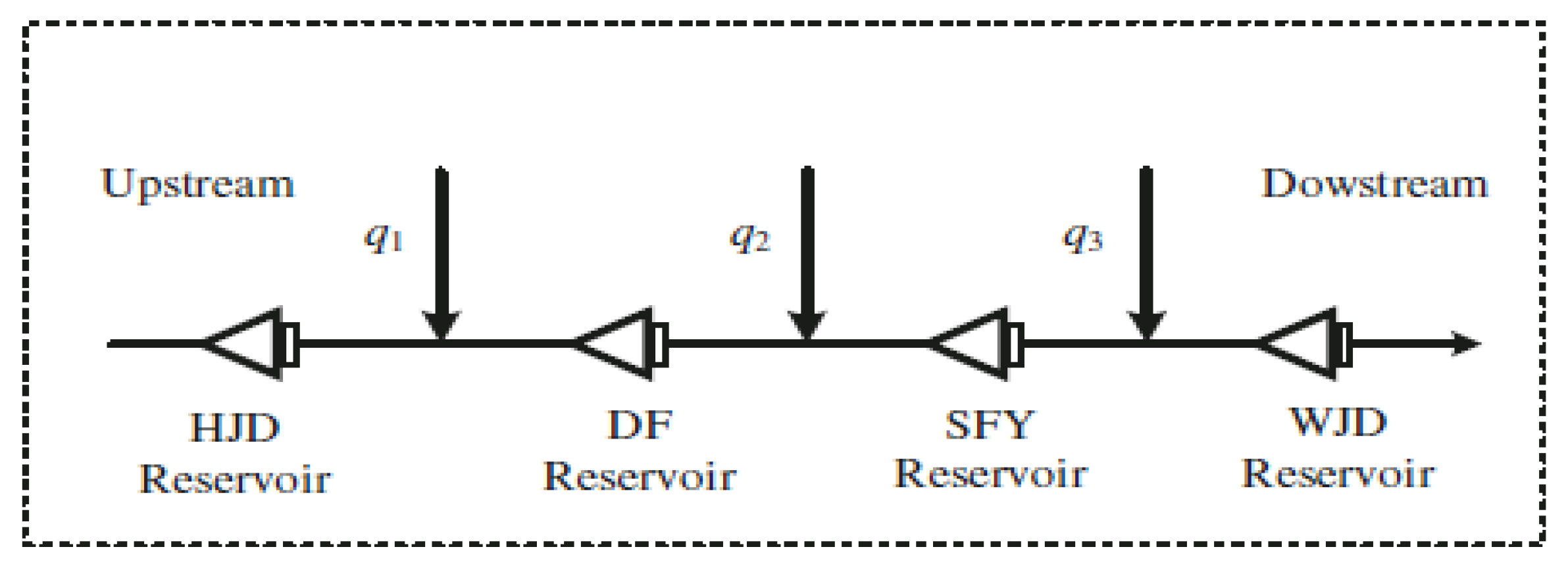
4. Case Study

The Wujiang multireservoir system is in the Wujiang Basin, and the Wujiang River is in southwest China. The area of this basin is 87,900 km², and the precipitation rate for this basin varies from 900 to 1400 mm. This system is one of 13 global systems that produce hydropower, and there are four hydropower reservoirs in this system. The water level reflects the reservoir storage, and thus the variation of outflow is affected by the fluctuation of the water level. When the water level was determined, the storage capacity could be calculated, and hence the outflow (water release) from the reservoir could be computed by continuity and the state equation. Figure 2 shows the multireservoir system where q₁, q₂, and q₃ represent the inflow for each reservoir.

The SFY reservoir has small regulatory storage. Thus, the optimization process was implemented on other reservoirs.

Table 1. Futures of the multireservoir system.

Reservoir Item	Unit	SFY	HJD	DF	WJD
Normal water level	m	385	150	345	502
Dead-storage water level	m	822	1076	936	720
Total storage	billion m3	0.2	4.5	0.9	2.1
Regulation storage	-	daily	multiyear	seasonal	seasonal
Power coefficient	-	8.5	8.5	8.35	8.17

presents various characteristics for all reservoirs in this study, such as the normal water level, dead water level, total storage, regulation storage, and power efficiency. It is noticeable that there is different regulation storage in the presented reservoirs: SFY has daily regulation, DF and WJD are regulated seasonally, while there is multiyear regulation for HJD. The main duty of the DF reservoir is hydropower generation, where the normal water level is 345 m, and the dead water level is 936 m. The efficiency of this hydropower plant is 8.35. The SFY reservoir has a storage of approximately 0.2 billion m³ and is downstream of the DF reservoir: The hydraulic head of the DYF is 936 m due to low storage in the reservoir. The capacity for the WJD hydropower plant is 1250 MW: The normal water level for this reservoir is 502 m, and the dead water level for this reservoir is 720 m. The total hydropower output from the system should be 680 MW to guarantee downstream demands. The inflow value for the reservoirs and the interzone for different climate conditions (wet, normal, and dry) are mentioned in

Table 2. Inflow to reservoir for different climate conditions.

Interval	Wet Year (m3/s)				Normal Year (m3/s)				Dry Year (ms/s)
	HJD	H-D	D-S	S-W	HJD	H-D	D-S	S-W	HJD	H-D	D-S	S-W
1	140	179	89	50	88	159	111	57	143	331	93	137
2	291	393	113	196	482	538	240	230	123	256	61	82
3	438	602	150	250	444	616	180	320	330	720	290	210
4	467	643	60	190	154	149	53	25	171	230	35	60
5	198	182	34	45	206	204	40	63	86	146	18	23
6	186	191	106	65	84	86	14	16	143	136	16	72
7	94	72	37	79	74	75	20	37	81	123	62	33
8	76	59	30	51	46	47	11	39	58	100	46	39
9	58	37	18	26	37	39	10	6	47	44	19	39
10	45	30	13	15	41	34	9	34	52	44	19	43
11	39	25	11	11	42	31	5	12	46	39	14	48
12	51	27	10	12	48	44	9	24	114	136	102	135
Average	173	203	56	82	146	168	58	72	116	192	65	77

Notes: H-D represents the interzone flow between the HJD reservoir and DF reservoir, D-S represents the interzone flow between the DF reservoir and SYF reservoir, and S-W represents the interzone flow between SYF and WJD.

. Additionally, the outflow for the WJD reservoir should be more than 100 m³/s due to navigation safety. The power coefficient in Table 1 was used to determine the efficiency of the entire turbine power system.

Dry years (May 1963–April 1964), wet years (May 1951–April 1952), and normal years (May 1985–April 1986) were considered different scenarios in the operation of the multireservoir system. The aim of the problem was to maximize hydropower production for the multireservoir system. Three years for each scenario were considered to examine the performance of the proposed algorithm for different conditions, because it was important that the method could manage the basin for the years with a scarcity of water resources.

The generated hydropower is dependent on the hydraulic head and turbine release, and both parameters were computed by determining the water level of the reservoirs. The outflows for the reservoirs were computed when the upstream water level was determined, and Equation (6) was used for computing the outflow when considering the spillway and turbine release. The outflow from each reservoir was considered to be the inflow into the downstream reservoir: When the outflow increased, the water level increased downstream, which caused a lower hydraulic head. The objective function was computed based on Equation (7) [26]:

$$\begin{array}{l}{V}_{m,t+1}=V_{m,t}+\eta \left(I_{m,t}-Q_{m,t}\right)\\ I_{m+1,t}=I{Q}_{m+1,t}+Q_{m,t-{\tau }_m}\end{array}$$

(6)

Equation (9) is a continuity equation, where $V_{m,t+1}$ is storage for the mth reservoir at time t + 1, $Q_{m,t}$ is the outflow of the mth reservoir, which includes the turbine release and spillway release, $I{Q}_{m+1,t}$ is the internal inflow into the m + 1 reservoir, ${\tau }_m$ is the routed outflow from the mth reservoir into the m + 1 reservoir downstream, $\eta$ is the conversion coefficient, and $I_{m+1,t}$ is the inflow into the m + 1 reservoir. Equation (7) is

$$\begin{array}{c}F=\max {\displaystyle {\displaystyle \sum }_{t-1}^T}{\displaystyle {\displaystyle \sum }_{m-1}^M}{N}_{m,t}\Delta T\\ N_{m,t}=k_m{q}_m{h}_{m,t}\end{array}$$

(7)

where F is an objective function (kwh), T is the number of operational periods, M is the number of hydropower plants, $N_{m,t}$ is the output hydropower for the mth hydropower plant (MW), $\Delta T$ is the time interval, $k_m$ is the hydropower plant coefficient, $q_m$ is the release passing turbines, and $h_{m,t}$ is the hydraulic head. The following constraints are considered for this problem [26]:

$${\underset{\_}{N}}_{m,t}\le N_{m,t}\le {\overline{N}}_{m,t}.$$

(8)

Equation (8) represents the constraint for each hydropower plant, where ${\underset{\_}{N}}_{m,t}$ is the lower and ${\overline{N}}_{m,t}$ is the upper output for the mth hydropower plant. Equation (9) is

$$N_{-t}\le N_{m,t}\le {\overline{N}}_t.$$

(9)

Equation (9) represents the constraint related to the total output of the system, where ${\underset{\_}{N}}_t$ and ${\overline{N}}_t$ represent the lower and upper outputs of the system, respectively. Equation (10) is

$$Z_{-mt}\le Z_{m,t}\le {\overline{Z}}_{mt}.$$

(10)

Equation (10) is related to the water level of each reservoir, where ${\underset{\_}{Z}}_{m,t}$ and ${\overline{Z}}_{m,t}$ represent the lower and upper levels of the reservoirs, respectively. Equation (11) is

$$Q_{-mt}\le Q_{m,t}\le {\overline{Q}}_{mt}$$

(11)

Equation (11) is considered to be one constraint for the outflow, where ${\underset{\_}{Q}}_{m,t}$ and ${\overline{Q}}_{m,t}$ represent the lower and upper outflows of the reservoirs, respectively. Equation (12) is

$$Z_{m,1}=Z_{m,b},Z_{m,T+1}=Z_{m,e}$$

(12)

Equation (12) is considered to be the boundary constraint, where $Z_{m,b}$ is the water level at the beginning of the operation period, and $Z_{m,e}$ is the water level at the end of the operation period.

If the constraints are not satisfied, penalty functions are added to the objective function:

$$F=-{\displaystyle {\displaystyle \sum _{t=1}^T}\left({\displaystyle {\displaystyle \sum _{m=1}^M}{N}_{m,t}-\delta {\left({\underset{\_}{N}}_t-{\displaystyle {\displaystyle \sum _{m=1}^M}{N}_{m,t}}\right)}^2}\right)}\Delta t,$$

(13)

where $\delta =\left[\begin{array}{l}1,{\displaystyle {\displaystyle \sum _{m=1}^M}{N}_{m,t}}\le {\underset{\_}{N}}_t\\ 0,{\displaystyle {\displaystyle \sum _{m=1}^M}{N}_{m,t}\ge {\underset{\_}{N}}_t}\end{array}\right]$. Equation (14) is

$$N_{m,t}=\left[\begin{array}{l}{p}_1\left(q_{m,t}-{\underset{\_}{q}}_{m,t}\right),q_{m,t}\in \left(-\infty ,{\underset{\_}{q}}_{m,t}\right)\\ k_m{q}_{m,t}{h}_{m,t},q_{m,t}\in \left({\underset{\_}{q}}_{m,t},{\overline{q}}_{m,t}\right)\\ p_2\left({\overline{q}}_{m,}t-q_{m,t}\right),q_{m,t}\in \left({\overline{q}}_{m,t},+\infty \right)\end{array}\right].$$

(14)

$N_{m,t}$ represents the hydropower output for each period, and p₁ and p₂ are penalty coefficients.

The following indexes are used to evaluate the hydropower output based on the CA [6]:

• The temporal reliability index. This index shows the number of periods where the generated hydropower is greater than the hydropower plant capacity. A high percentage for this index is suitable:

  $$TR=\frac{N_{t=1}^T\left(N_{m,t}\ge PP{C}_m\right)}{T}\times 100,$$

  (15)

  where $TR$ is the temporal reliability index, $N_{t=1}^T\left(N_{m,t}\ge PP{C}_m\right)$ is the number of periods where the generated hydropower is greater than the hydropower plant capacity, $PP{C}_m$ is the hydropower plant capacity, and T is the total number of operational periods;
• Volumetric reliability index. This index shows the percentage of generated hydropower compared to the producible maximum hydropower at each hydropower plant. A high percentage of this index shows that the algorithm could generate the required hydropower for downstream demands [6]:

  $$VR=\frac{N_{t=1}^T\left(\left({\mathrm{N}}_{m,t}|N_{m,t}<PP{C}_m\right)\vee \left(\mathrm{PP}{\mathrm{C}}_m|{\mathrm{N}}_{m,t+1}\ge PP{C}_m\right)\right)}{T.PPC}\times 100,$$

  (16)

  where VR is the volumetric reliability index, $N_{t=1}^T\left(\left(N_{m,t}|N_{m,t}<PP{C}_m\right)\vee \left(PP{C}_m|N_{m,t+1}<PP{C}_m\right)\right)$ is the total generated hydropower during the operational periods, and $T.PPC$ is the maximum generated hydropower;
• Vulnerability index. The average amount of failure occurrences in the system is measured by the vulnerability index. The average hydropower deficits are measured by the vulnerability index:

  $$V=\frac{{\displaystyle {\displaystyle \sum _{t=1}^T}\left[\left(PP{C}_m-N_{m,t}|N_{m,t}<PP{C}_m\right)\vee \left(0|N_{m,}{}_t\ge PPC\right)\right]}}{T},$$

  (17)

  where ${\displaystyle {\displaystyle \sum _{t=1}^T}\left[\left(PP{C}_m-N_{m,t}|N_{m,t}<PP{C}_m\right)\vee \left(0|N_{m,}{}_t\ge PPC\right)\right]}$ is the total hydropower deficit;
• RMSE (root mean square error). The root mean square error between the generated hydropower and hydropower point capacity, as shown by Equation (18). A low value for this index represents better performance of the algorithm based on more generated hydropower:

  $$RMSE=\sqrt{{\displaystyle {\displaystyle \sum _{t=1}^T}\frac{{\left(PP{C}_m-N_{m,t}\right)}^2}{T}}};$$

  (18)
• MAE (mean absolute error). The mean absolute error between the generated hydropower and hydropower plant capacity, which is measured based on the following equations. A low value for this index is suitable and shows a reduced deficit:

  $$MAE={\displaystyle {\displaystyle \sum _{t=1}^T}\frac{\left|PP{C}_m-N_{m,t}\right|}{T}}.$$

  (19)

The mathematical model for multireservoir operation is considered based on the following criteria:

• The water level for the multireservoir system is considered to be the decision variable, and the initial position of the crows is considered based on the water level;
• The continuity equation is used to compute the outflow based on Equation (9);
• Different constraints are checked: If these constraints are not satisfied, the penalty functions are used;
• The objective function is computed for each member based on Equation (13);
• The number of operational periods (m) is compared to the total number of periods (M). If this is satisfied, go to the next level. Otherwise, return to the second step;
• The decision variables or crow positions are updated based on Equations (1) and (2);
• The memories of crows are updated based on Equation (5);
• The convergence criterion is checked. If it is satisfied, the algorithm finishes. Otherwise, the algorithm returns to the second step.

5. Results and Discussion

5.1. Sensitivity Analysis

The evolutionary algorithms had random parameters, with values that had to be initialized at the beginning before applying them to the real case study. Therefore, a sensitivity analysis was considered for the near-accurate determination of these parameters. In fact, the sensitivity analysis could be carried out to study the variation in the objective function of the system versus the variation in the initial values of the algorithm’s parameters. Several trial and error procedures were carried out to examine the proper initial values for the algorithm’s parameters. For example, in cases where the main target was used to maximize hydropower production, the procedure was identifying a particular range for the domain of the parameter values. In this research, several trial and error procedures were performed. First, the population was changed for the constant values of two other parameters. Second, the other values of other parameters were changed versus constant population size.

As seen in

Table 3. Sensitivity analysis for different algorithms for dry years, normal years, and wet years.

Dry Year
Population Size	Objective Function (108 kwh)	$f{l}^{i,iter}$	Objective Function (108 kwh)	$A{P}^{i,iter}$	Objective Function (108 kwh)
20	101.78	1	100.45	0.10	100.67
40	102.54	2	101.23	0.20	101.11
60	101.99	3	102.54	0.30	102.54
80	101.01	4	101.01	0.40	100.02
Normal Year
Population Size	Objective Function (108 kwh)	$f{l}^{i,iter}$	Objective Function (108 kwh)	$A{P}^{i,iter}$	Objective Function (108 kwh)
20	104.54	1	104.89	0.10	104.57
40	105.59	2	105.12	0.20	105.58
60	106.20	3	106.23	0.30	106.24
80	105.57	4	104.45	0.40	105.59
Wet Year
Population Size	Objective Function (108 kwh)	$f{l}^{i,iter}$	Objective Function (108 kwh)	$A{P}^{i,iter}$	Objective Function (108 kwh)
20	124.45	1	123.69	0.10	123.67
40	125.78	2	124.58	0.20	125.78
60	124.69	3	125.78	0.30	124.58
80	123.12	4	124.49	0.40	124.49

, a normal year was considered, and changes in the population size ranging from 20 to 80 were considered. It could be found that when the population size was 60, the objective function had a maximum value. In other words, to achieve an optimal value of the objective function, it was recommended to initialize the value of the population size to be equal to 60. In the same fashion, the flight length ($f{l}^{i,iter}$) for the normal year changed from 1 to 4, and the maximum value for the objective function was 106.23 (10⁸ kwh). From Table 3, the best initialization value for the flight length might have been equal to 3. The range of changes in the awareness probability ($A{P}^{i,iter}$) was selected to be between 0.10 and 0.40. The maximum value for the objective function, 106.24 (10⁸ kwh), occurred when the initial value of this parameter might have been equal to 0.30. A complete sensitivity analysis for all other cases of dry and wet years were carried out in a similar sequence, and all of the best initial values for the algorithm’s parameters are presented in Table 3.

5.2. Ten Random Results for Different Algorithms

Table 4. Power production for dry years, normal years, and wet years. CA: Crow algorithm; MBF: Monarch butterfly; GA: Genetic algorithm; PSO: Particle swarm optimization.

Dry Year
Run	CA (108 kwh)	MBF (108 kwh) [26]	GA (108 kwh) [26]	PSO (108 kwh) [26]
1	102.54	101.45	97.84	100.20
2	102.53	101.44	98.45	100.24
3	102.53	101.45	98.72	100.18
4	102.54	101.45	98.37	100.26
5	102.54	101.45	98.97	100.23
6	102.54	101.45	99.19	100.23
7	102.54	101.45	99.29	100.33
8	102.54	101.45	99.04	100.22
9	102.54	101.45	99.10	100.21
10	102.54	101.45	99.07	100.19
Average	102.54	101.45	98.06	100.18
Variation coefficient	0.0003	0.00003	0.716	0.065
Time (s)	23	26	32	29
Normal Year
Run	CA (108 kwh)	MBF (108 kwh) Ehteram et al. [26]	GA (108 kwh) Ehteram et al. [26]	PSO (108 kwh) [26]
1	106.20	105.22	104.15	104.16
2	106.19	105.22	104.15	104.16
3	106.20	105.23	104.07	104.25
4	106.20	105.23	104.15	104.18
5	106.20	105.23	103.58	104.22
6	106.20	105.23	103.87	104.24
7	106.20	105.23	104.71	104.07
8	106.20	105.23	103.11	104.34
9	106.20	105.23	103.99	104.32
10	106.20	105.23	104.16	104.12
Average	106.20	105.23	103.98	104.22
Variation coefficient	0.0002	0.0003	0.201	0.083
Time (s)	24	29	35	32
Wet Year
Run	CA (108 kwh)	MBF (108 kwh) [26]	GA (108 kwh) [26]	PSO (108 kwh) [26]
1	125.77	124.12	122.58	123.11
2	125.77	124.11	122.58	123.11
3	125.78	124.11	122.20	123.11
4	125.78	124.12	122.61	123.11
5	125.78	124.12	122.57	122.67
6	125.78	124.12	122.18	123.11
7	125.78	124.12	122.46	122.95
8	125.78	124.12	122.69	122.91
9	125.78	124.12	122.65	123.11
10	125.78	124.12	122.53	123.11
Average	125.78	124.12	122.47	123.01
Variation coefficient	0.00003	0.00003	0.195	0.147
Time (s)	23	25	31	29

shows the 10 random results for the different evolutionary algorithms based on normal years, wet years, and dry years. The average generated hydropower energy for the CA based on normal years was 106.20 (10⁸ kwh), with values of 105.23, 103.98, and 104.22 (10⁸ kwh) via the MBF, GA, and PSO, respectively. The average generated energy for normal years based on the CA was 0.94%, 2.09%, and 1.8% greater than via the MBF, GA, and PSO, respectively. Additionally, the computational time for the CA based on normal years was 24 s, which was 17%, 25%, and 31% less than via the MBF, PSO, and GA, respectively. It can be observed that the results for the dry and wet years assured that the CA could achieve a better value for the objective function with a minimal computational time. The computational time for the CA based on dry years was 23 s, which was 11.5%, 20%, and 28% less than via the MBF, GA, and PSO, respectively. The lowest computation time consumed refers to fast convergence: Also, this reduction occurred when the number of evaluations for the CA was less than other algorithms.

The variation coefficient for the CA for all years was a small value, which proved that one computer run was reliable and proved the solution to be of high quality. The used computerized system for this research and the one used in Reference [26] by the authors are similar systems (PCs with i5 CPU 2.4 GHz, ram/500 GB HDD).

5.3. Evaluation of Different Algorithms Based on Computed Indexes

Table 5. Computed indexes for generated power for dry years, normal years, and wet years. RMSE: Root mean square error; MAE: Mean absolute error.

HJD (Dry Year)
Method	Temporal Reliability Index	Volumetric Reliability Index	Vulnerability Index	RMSE MW	MAE MW
CA	38%	91%	20%	1.4 MW	1.2 MW
MBF	25%	83%	34%	2.3 MW	2.1 MW
PSO	18%	76%	39%	3.4 MW	3.2 MW
GA	14%	65%	41%	3.9 MW	3.6 MW
SFY (Dry Year)
CA	32%	90%	22%	1.6 MW	1.2 MW
MBF	29%	82%	36%	2.5 MW	2.3 MW
PSO	27%	75%	41%	3.6 MW	3.4 MW
GA	24%	63%	43%	4.1 MW	4.0 MW
DF (Dry Year)
CA	39%	92%	19%	1.2 MW	1.1 MW
MBF	27%	83%	32%	2.3 MW	2.1 MW
PSO	22%	77%	41%	3.1 MW	3.0 MW
GA	16%	67%	43%	3.9 MW	3.7 MW
WJD (Dry Year)
CA	41%	91%	19%	1.4 MW	1.2 MW
MBF	29%	84%	32%	2.1 MW	2.0 MW
PSO	19%	77%	40%	3.1 MW	3.0 MW
GA	16%	66%	42%	3.6 MW	3.4 MW
HJD (Normal Year)
Method	Temporal Reliability Index	Volumetric Reliability Index	Vulnerability Index	RMSE MW	MAE MW
CA	42%	92%	17%	1.2 MW	9.0 MW
MBF	39%	91%	22%	1.5 MW	1.3 MW
PSO	27%	85%	28%	2.4 MW	2.0 MW
GA	29%	76%	31%	2.9 MW	2.6 MW
SFY (Normal Year)
CA	41%	91%	21%	1.3 MW	1.2 MW
MBF	38%	84%	29%	1.9 MW	1.4 MW
PSO	27%	82%	32%	2.8 MW	2.6 MW
GA	24%	75%	35%	2.6 MW	2.1 MW
DF (Normal Year)
CA	41%	92%	20%	1.3 MW	1.0 MW
MBF	35%	87%	24%	1.5 MW	1.4 MW
PSO	29%	81%	29%	2.3 MW	2.1 MW
GA	28%	79%	32%	2.9 MW	2.6 MW
WJD (Normal Year)
CA	42%	93%	17%	1.2 MW	1.2 MW
MBF	33%	92%	22%	1.6 MW	1.5 MW
PSO	26%	85%	26%	2.1 MW	1.9 MW
GA	30%	79%	28%	2.6 MW	2.4 MW
HJD (Wet Year)
Method	Temporal Reliability Index	Volumetric Reliability Index	Vulnerability Index	RMSE MW	MAE MW
CA	46%	95%	15%	0.90 MW	1.0 MW
MBF	42%	93%	16%	1.3 MW	1.2 MW
PSO	35%	89%	18%	1.6 MW	2.1 MW
GA	32%	80%	20%	1.8 MW	2.7 MW
SFY (Wet Year)
CA	42%	93%	22%	1.2 MW	1.1 MW
MBF	40%	85%	28%	1.6 MW	1.4 MW
PSO	29%	84%	30%	2.5 MW	2.3 MW
GA	26%	77%	34%	2.2 MW	2.0 MW
DF (Wet Year)
CA	47%	96%	19%	0.80 MW	0.95 MW
MBF	43%	94%	21%	1.1 MW	1.0 MW
PSO	36%	92%	20%	1.5 MW	1.4 MW
GA	34%	90%	24%	1.9 MW	1.8 MW

shows the comparison between generated hydropower and producible maximum hydropower (i.e., power plant capacity). The dry years were the most critical years, and the HJD hydropower plant was selected to analyze the results to avoid repetition. Thus, all of the mentioned analysis is for the HJD reservoir, hydropower plant, and dry years, and the results were the same for other years and hydropower plants.

The temporal reliability index (TRI) for the CA based on dry years was 38%, which was 13%, 20%, and 24% more than via the MBF, PSO, and GA, respectively. The percent of this index represents the number of periods where the hydropower exceeded the set threshold (i.e., power plant capacity). Thus, there were no hydropower deficits during these periods due to a surplus of hydropower generation.

When the TRI had a higher value, the system could generate hydropower for more periods, with a surplus capacity comparable to the hydropower plant capacity. Additionally, the volumetric reliability index (VRI) based on the CA during dry years was 91%, which was 8%, 15%, and 26% more than via the MBF, PSO, and GA, respectively. This result showed that the generated hydropower via the CA for more periods was closer to the hydropower plant capacity compared to via the MBF, GA, and PSO.

The vulnerability index for the CA based on dry years was 20%, which was 14%, 19%, and 21% less than via the MBF (monarch butterfly algorithm), PSO, and GA, respectively. In fact, a smaller value for this index based on the CA during dry years showed that the intensities of failure occurrences or hydropower deficits via the CA were less than via the MBF, PSO, and GA. The RMSE for the CA based on dry years was 1.4 MW, which was 39%, 58%, and 64% less than via the MBF, PSO, and GA, respectively, when the generated hydropower was compared to hydropower plant capacity.

Additionally, the MAE for the CA based on dry years was 1.2 MW, which was 42%, 62.5%, and 66% less than via the MBF, PSO, and GA, respectively. Thus, the MAE and RMSE showed that the CA could generate hydropower similar to the hydropower plant capacity. The comparison of results for the CA and other algorithms during other years also affirmed the improved performance of the CA. Another point was related to the values of different indexes during different years. For example, the TRI and VRI for wet years had the greatest values compared to other years.

The VRI was 95% based on wet years for the HJA reservoir via the CA, and it was 92% and 91% for normal and dry years, respectively. All indexes during wet years had more acceptable values based on all algorithms when compared to the same algorithms during normal and dry years for all hydropower plants, which was due to more water resources for the multireservoir system during wet years. The conditions for the MBF, PSO, and GA based on dry years for all hydropower plants were more critical compared to during wet and normal years. Therefore, the values of the TRI and VRI decreased, and the RMSE and MAE increased significantly during dry years compared to during other years.

For example, the TRI via the CA during dry years for the HJD hydropower plant decreased by 4% and 6% compared to normal and wet years, respectively, while it decreased during dry years at the HJD hydropower plant via the GA when compared to normal and wet years (15% and 18%, respectively). Additionally, other indexes, such as the MBF, GA, and PSO (based on dry years), had the same conditions. Thus, the PSO, GA, and MBF were more vulnerable compared to the CA when there were limited water resources during some years. Although the GA and PSO algorithms have shown a relatively good performance in previous research, the CA in this research achieved an outstanding performance better than them. This might have been due to the fact that PSO and GAs have been examined for single reservoir water systems with single objectives and have been evaluated using traditional performance indexes. In addition, the major difference in exploring the weaknesses of the GA and PSO algorithms compared to the CA is that both algorithms (GA and PSO) have been applied only for normal average climate conditions, without paying attention to the possibility of experiencing wet and dry climate conditions.

Comprehensive evaluations were carried out. In fact, several multicriteria decision models could be used for the selection of the best method. If x_ij is considered the value of the index in Table 4 for each method, a multicriteria decision model can predicate the ranks for different methods based on the following steps: (1) The consideration and definition of the suitable indexes for evaluating different methods; (2) the allocation of weight to the index, where the vulnerability, reliability, RMSE, and MAE based on the same importance have the same weight for this study; and (3) the prioritization of different methods based on different indexes.

The dry year as a critical condition was selected, and compromise programming (CP) was used as a multidecision model for four reservoirs to select the best model based on the mentioned indexes in Table 4 [9]:

$$L_p\left(S_i\right)={\left[{\displaystyle {\displaystyle \sum _{j=1}^n}{\left(\frac{x_j^{+}-x_{ij}}{x_j^{+}-x_j^{-}}\right)}^p}\right]}^{\frac{1}{p}},$$

(20)

where $L_p\left(S_i\right)$ is the distance of a solution from the ideal solution; and $x_j^{+}$ and $x_j^{-}$ are, respectively, the ideal solution (the most value for maximizing criteria or lowest value for minimizing criteria) and the negative ideal (the most value for minimizing criteria or lowest value for maximizing criteria). Three values for p were selected for this model to evaluate distances (p = 1, p = 2, and $p=\infty$) as black distance, Euclidean distance, and Tchebycheff distance [26]. The multicriteria decision gave ranks to the method for different reservoirs based on the mentioned values of indexes. The results indicated that the CA method based on RMSE, MAE, the reliability index, and the vulnerability index received the first rank, and MBF, PSO, and GA received other ranks. The ranks showed that the CA based on all indexes had the best rank, and the MBF acted based on the next alternative.

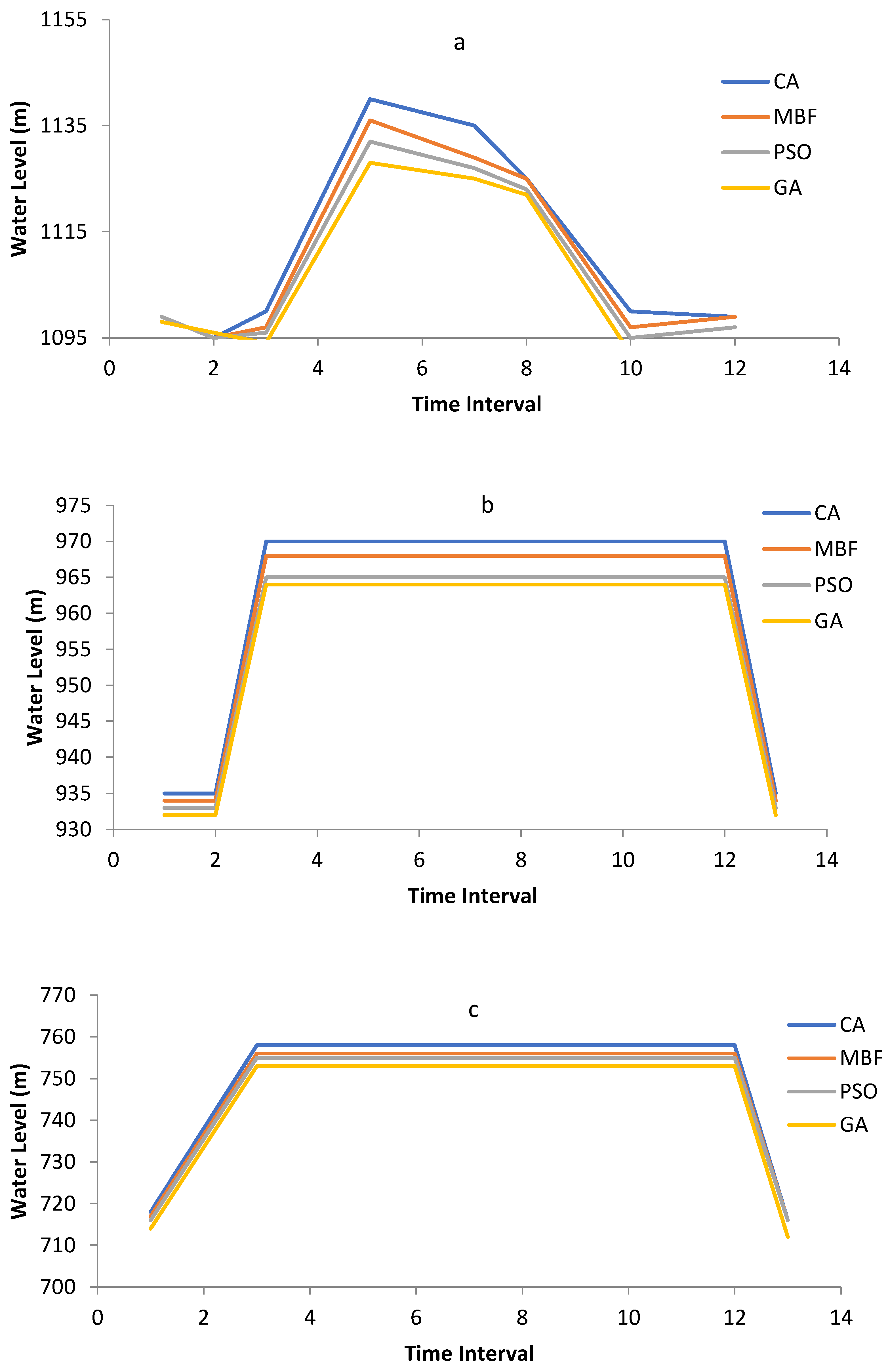
5.4. Rationality of Operating the Multireservoir System

A dry year was selected as the critical year for the hydraulic and logical analyses to avoid repeating the results of this section. Figure 3 shows that the water levels for WJD, DF, and HJD varied based on the CA during different periods. The inflow into the HJD reservoir during dry years had an initial interval of 88 m³/s (Table 2): This value was small, and if the system wants to meet the minimum required hydropower (680 MW), the outflow from the HJD reservoir should increase, which would allow the downstream reservoirs to have enough inflow for hydropower generation.

Thus, the water level decreased in this reservoir, and the water level for the other reservoirs increased to reach a normal level (Figure 3). In fact, the value of the inflow into the HJD reservoir was small during the initial time interval, and the value of the inflow into the HJD reservoir increased to reach a normal water level (1140 m). The outflow from the HJD reservoir increased, which did not cause a real shortage for the downstream reservoirs: Thus, the water level decreased in the HJD reservoir to keep the water level under normal conditions for the downstream reservoirs. The water level for the reservoirs after the HJD reservoir did not decrease until the final period (Figure 3).

Table 6. Outflow, hydraulic head, and power output, optimized by CA, for the studied reservoirs.

Interval	Outflow (m3/s)				Hydraulic Head (m)				Power Output (MW)				Total Power (MW)
	HJD	DF	SFY	WJD	HJD	DF	SFY	WJD	HJD	DF	SFY	WJD	-
1	118.6	277.9	389.4	100.12	121.4	102.3	69	112.4	120.4	235.3	226.3	90.4	725.7
2	0.0	351.4	592.3	675.2	132.5	114.22	69	122.2	0.0	332.4	344.2	690.4	1367.10
3	0.20	612.2	795.3	1084.2	145.7	125.46	69	130.5	0.5	652.4	463.7	1161.3	2277.9
4	111.0	254.2	312.2	333.1	161.3	127.23	69	125.2	151.2	275.8	181.3	367.7	976.40
5	201.2	406.9	447.6	511.4	155.2	126.22	69	132.2	275.34	434.9	259.3	552.3	1521.84
6	107.4	195.3	209.3	224.1	161.2	127.31	69	134.7	145.21	211.2	121.3	244.66	722.37
7	145.21	222.3	243.1	277.11	157.4	125.30	69	134.2	200.22	221.7	139.1	305.4	866.40
8	205.54	251.1	265.2	303.3	154.22	129.12	69	132.2	261.31	261.4	156.2	331.22	1010.13
9	227.11	265.3	276.2	275.2	145.21	127.12	69	129.4	275.31	286.3	154.2	308.14	1023.95
10	242.65	281.2	289.1	322.2	137.76	124.12	69	126.2	290.21	301.1	166.3	350.12	1107.73
11	301.11	331.1	337.2	351.1	122.1	125.4	69	124.2	302.12	355.6	197.3	380.23	1238.23
12	60.28	293.2	302.1	841.2	124.2	122.4	69	116.3	65.21	278.2	172.3	808.6	1331.60

shows more details for the reservoirs and hydropower plants based on the CA. The outflow for the WJD during all periods was more than 100 m³/s based on Table 6: Thus, navigation security was considered for the WJD reservoir. The total hydropower output for all periods was more than 680 MW: Thus, the smallest amount of required hydropower was well supplied. Additionally, the variation in hydraulic heads during the wet seasons had an increasing trend, and it had a decreasing trend during the dry seasons, which is consistent with Figure 3. Additionally, the hydropower outputs for HJD were close to zero, because the inflow value for the HJD reservoir during these two periods was considerable: Thus, the reservoir should increase the storage value during critical periods, such as dry seasons. Therefore, the outflow of hydropower generation for the HJD reservoir decreased during these periods. Finally, the hydraulic head increased, and there was enough storage for critical periods.

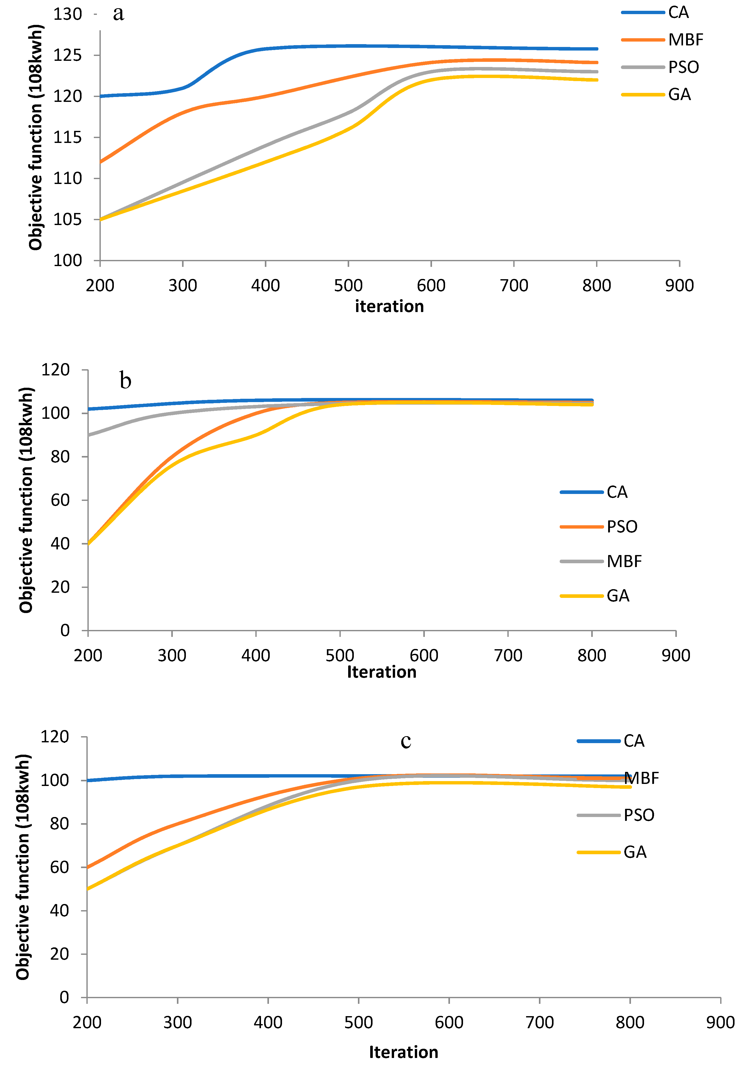
5.5. Convergence Curves

Figure 4 shows the convergence for three years. The results indicate that the CA converged toward more energy produced than other algorithms based on a smaller number of iterations. For example, the CA converged to 106.20 (10⁸ kwh) after 400 iterations during normal years, while the PSO, GA, and MBF converged after 500 iterations. Thus, the CA could achieve an optimal performance goal based on a smaller number of iterations during the optimization process. The parameters for the other methods computed were based on sensitivity analysis, such as CA. For example, the population size for PSO, CA, and MBF was 80, 60, and 30. The mutation probability for the GA was 0.10, and the crossover probability for the GA was 0.5. The inertia coefficient for PSO was 0.8, and the acceleration coefficient for PSO was 2.

6. Conclusions

The present study considered the operation of a multireservoir system with the aim of increasing hydropower generation based on a new, evolutionary CA. Based on the proposed model, the average generated energy for normal years was 0.94%, 2.09%, and 1.8% more than via the MBF, GA, and PSO, respectively. The average generated energy for wet years based on the CA was 1.3%, 2.6%, and 2.2% more than via the MBF, GA, and PSO, respectively. The computational time based on the CA over three years was less than via the GA, PSO, and MBF. The results indicated that the CA could supply the required hydropower for downstream demand based on high values of the TRI and VRI. For example, the VRI via the CA for the HJA reservoir was 91%, while it was 83%, 76%, and 65% via the MBF, PSO, and GA, respectively. Additionally, the CA decreased the vulnerability index compared to the MBF, PSO, and GA for all reservoirs. The results indicated that the HJD reservoir had an important role in the process of hydropower generation: Therefore, the inflow volume into this reservoir had considerable value when storing flow during critical periods. Additionally, the reservoir with an increase in outflow attempted to transfer the necessary inflow toward downstream reservoirs for hydropower generation. Thus, the CA has high potential for water resource and energy management based on the computed results: Also, future studies can be related to the operation of a multireservoir system under climate change conditions based on the CA to determine the ability of the CA under climate change conditions when managing and planning in water resource and energy fields.

References

1. Nordenstam, L.; Djuric Ilic, D.; Ödlund, L. Corporate greenhouse gas inventories, guarantees of origin and combined heat and power production—Analysis of impacts on total carbon dioxide emissions. J. Clean. Prod. 2018, 186, 203–214. [Google Scholar] [CrossRef]
2. Manokar, A.M.; Winston, D.P.; Kabeel, A.E.; Sathyamurthy, R. Sustainable fresh water and power production by integrating PV panel in inclined solar still. J. Clean. Prod. 2018, 172, 2711–2719. [Google Scholar] [CrossRef]
3. Shrouf, F.; Gong, B.; Ordieres-Meré, J. Multi-level awareness of energy used in production processes. J. Clean. Prod. 2017, 142, 2570–2585. [Google Scholar] [CrossRef]
4. Fan, J.L.; Hu, J.W.; Kong, L.S.; Zhang, X. Relationship between energy production and water resource utilization: A panel data analysis of 31 provinces in China. J. Clean. Prod. 2018, 167, 88–96. [Google Scholar] [CrossRef]
5. Gong, X.; Van der Wee, M.; De Pessemier, T.; Verbrugge, S.; Colle, D.; Martens, L.; Joseph, W. Integrating labor awareness to energy-efficient production scheduling under real-time electricity pricing: An empirical study. J. Clean. Prod. 2017, 168, 239–253. [Google Scholar] [CrossRef] [Green Version]
6. Ehteram, M.; Karami, H.; Farzin, S. Reducing Irrigation Deficiencies Based Optimizing Model for Multi-Reservoir Systems Utilizing Spider Monkey Algorithm. Water Resour. Manag. 2018, 32, 2315–2334. [Google Scholar] [CrossRef]
7. Ehteram, M.; Karami, H.; Farzin, S. Reservoir Optimization for Energy Production Using a New Evolutionary Algorithm Based on Multi-Criteria Decision-Making Models. Water Resour. Manag. 2018, 32, 2539–2560. [Google Scholar] [CrossRef]
8. Babel, M.S.; Nguyen Dinh, C.; Mullick, M.R.A.; Nanduri, U.V. Operation of a hydropower system considering environmental flow requirements: A case study in La Nga river basin, Vietnam. J. Hydro-Environ. Res. 2012, 6, 63–73. [Google Scholar] [CrossRef]
9. Pimenta, F.M.; Assireu, A.T. Simulating reservoir storage for a wind-hydro hydrid system. Renew. Energy 2015, 76, 757–767. [Google Scholar] [CrossRef]
10. Jahandideh-Tehrani, M.; Bozorg Haddad, O.; Loáiciga, H.A. Hydropower Reservoir Management Under Climate Change: The Karoon Reservoir System. Water Resour. Manag. 2015, 29, 749–770. [Google Scholar] [CrossRef]
11. Arunkumar, R.; Jothiprakash, V. Chaotic Evolutionary Algorithms for Multi-Reservoir Optimization. Water Resour. Manag. 2013, 27, 5207–5222. [Google Scholar] [CrossRef]
12. Wu, Y.; Chen, J. Estimating irrigation water demand using an improved method and optimizing reservoir operation for water supply and hydropower generation: A case study of the Xinfengjiang reservoir in southern China. Agric. Water Manag. 2013, 116, 110–121. [Google Scholar] [CrossRef]
13. Chang, J.-x.; Bai, T.; Huang, Q.; Yang, D.W. Optimization of Water Resources Utilization by PSO-GA. Water Resour. Manag. 2013, 27, 3525–3540. [Google Scholar] [CrossRef]
14. Yang, T.; Gao, X.; Sellars, S.L.; Sorooshian, S. Improving the multi-objective evolutionary optimization algorithm for hydropower reservoir operations in the California Oroville-Thermalito complex. Environ. Model. Softw. 2015, 69, 262–279. [Google Scholar] [CrossRef]
15. Bozorg-Haddad, O.; Karimirad, I.; Seifollahi-Aghmiuni, S.; Loáiciga, H.A. Development and Application of the Bat Algorithm for Optimizing the Operation of Reservoir Systems. J. Water Resour. Plan. Manag. 2015, 141, 04014097. [Google Scholar] [CrossRef]
16. Haddad, O.B.; Moravej, M.; Loáiciga, H.A. Application of the Water Cycle Algorithm to the Optimal Operation of Reservoir Systems. J. Irrig. Drain. Eng. 2015, 141, 04014064. [Google Scholar] [CrossRef]
17. Haddad, O.B.; Hosseini-Moghari, S.-M.; Loáiciga, H.A. Biogeography-Based Optimization Algorithm for Optimal Operation of Reservoir Systems. J. Water Resour. Plan. Manag. 2016, 142, 04015034. [Google Scholar] [CrossRef]
18. Garousi-Nejad, I.; Bozorg-Haddad, O.; Loáiciga, H.A.; Mariño, M.A. Application of the Firefly Algorithm to Optimal Operation of Reservoirs with the Purpose of Irrigation Supply and Hydropower Production. J. Irrig. Drain. Eng. 2016, 142, 04016041. [Google Scholar] [CrossRef]
19. Ehteram, M.; Mousavi, S.F.; Karami, H.; Farzin, S.; Emami, M.; Binti Othman, F.; Amini, Z.; Kisi, O.; El-Shafie, A. Fast convergence optimization model for single and multi-purposes reservoirs using hybrid algorithm. Adv. Eng. Inform. 2017, 32, 287–298. [Google Scholar] [CrossRef]
20. Askarzadeh, A. A novel metaheuristic method for solving constrained engineering optimization problems: Crow search algorithm. Comput. Struct. 2016, 169, 1–12. [Google Scholar] [CrossRef]
21. Oliva, D.; Hinojosa, S.; Cuevas, E.; Pajares, G.; Avalos, O.; Gálvez, J. Cross entropy based thresholding for magnetic resonance brain images using Crow Search Algorithm. Expert Syst. Appl. 2017, 79, 164–180. [Google Scholar] [CrossRef]
22. Javidi, A.; Salajegheh, E.; Salajegheh, J. Enhanced crow search algorithm for optimum design of structures. Appl. Soft Comput. 2019, 77, 274–289. [Google Scholar] [CrossRef]
23. Liu, D.; Liu, C.; Fu, Q.; Li, T.; Imran, K.M.; Cui, S.; Abrar, F.M. ELM evaluation model of regional groundwater quality based on the crow search algorithm. Ecol. Indic. 2017, 81, 302–314. [Google Scholar] [CrossRef]
24. Abdelaziz, A.; Elhoseny, M.; Salama, A.S.; Riad, A.M. A machine learning model for improving healthcare services on cloud computing environment. Measurement 2018, 119, 117–128. [Google Scholar] [CrossRef]
25. Anter, A.M.; Hassenian, A.E.; Oliva, D. An improved fast fuzzy c-means using crow search optimization algorithm for crop identification in agricultural. Expert Syst. Appl. 2019, 118, 340–354. [Google Scholar] [CrossRef]
26. Ehteram, M.; Karami, H.; Mousavi, S.-F.S.-F.; Farzin, S.; Kisi, O. Optimization of energy management and conversion in the multi-reservoir systems based on evolutionary algorithms. J. Clean. Prod. 2017, 168, 1132–1142. [Google Scholar] [CrossRef]
Figure 1. Crow flowchart algorithm.
Applsci 09 02280 g001
Figure 2. The Wujiang multi-hydropower reservoirs (HJD, DF, SFY, and WJD).
Applsci 09 02280 g002
Figure 3. Water level for (a) HJD reservoir, (b) DF reservoir, and (c) WJD.
Applsci 09 02280 g003
Figure 4. The convergence curve for (a) wet years, (b) normal years, and (c) dry years.
Applsci 09 02280 g004