Article

Discrete and Phase Field Methods for Linear Elastic Fracture Mechanics: A Comparative Study and State-of-the-Art Review

1
Institute of Structural Engineering, D-BAUG, 8093 ETH Zurich, Switzerland
2
Centre for Structural Engineering and Informatics, Faculty of Engineering, The University of Nottingham, NG7 2RD Nottingham, UK
3
Centre for Additive Manufacturing, Faculty of Engineering, The University of Nottingham, NG7 2RD Nottingham, UK
*
Author to whom correspondence should be addressed.
Appl. Sci. 2019, 9(12), 2436; https://doi.org/10.3390/app9122436
Submission received: 31 March 2019 / Revised: 21 May 2019 / Accepted: 23 May 2019 / Published: 14 June 2019
(This article belongs to the Special Issue Computational Methods for Fracture)

Abstract

:
Three alternative approaches, namely the extended/generalized finite element method (XFEM/GFEM), the scaled boundary finite element method (SBFEM) and phase field methods, are surveyed and compared in the context of linear elastic fracture mechanics (LEFM). The purpose of the study is to provide a critical literature review, emphasizing on the mathematical, conceptual and implementation particularities that lead to the specific advantages and disadvantages of each method, as well as to offer numerical examples that help illustrate these features.

1. Introduction

The need for lighter, stronger, and resilient structures across multiple engineering domains, e.g., the aerospace, automotive, and construction industries, necessitates a robust, economical and high-fidelity simulation of failure processes [1,2,3]. Failure in structural components subjected to static and/or dynamic loading is commonly associated with complex phenomena, i.e., crack nucleation, propagation, branching, merging and arrest [4,5]. These phenomena emerge from micro-material discontinuities, which under the action of external stimuli accumulate to cracks and evolve across several length scales eventually leading to structural failure. From a computational standpoint, these physics of damage evolution have proven challenging to resolve.
Over the past 20 years, the eXtended Finite Element method (XFEM), the Scaled Boundary Finite Element method (SBFEM) and most recently the Phase Field method (PFM), have emerged as distinct methodologies with the common objective of resolving fracture propagation. In this work, we provide a comparative platform for these methodologies pertinent to both the mathematical treatment of damage evolution and the corresponding algorithmic implications within the framework of Linear Elastic Fracture Mechanics (LEFM).
LEFM methods describe damage initiation and propagation within the remit of brittle and quasi-brittle material response. LEFM has been traditionally treated within two distinct methodological frameworks, i.e.,  computational fracture mechanics (see, e.g., [6]) and continuum damage mechanics (see, e.g., [7]). In the former, damage is explicitly defined as a discrete topological discontinuity. In the latter, damage is effectively homogenised over a representative volume. Diffuse crack approaches effectively lie in the boundary of the two aforementioned methods. The need to predict damage related phenomena precisely, accurately, and economically within the context of LEFM has spurred research into an extensive suite of alternative methodologies.
The finite element method (FEM), a representative of the discrete methods class, has reached a mature development status, effectively becoming the industry standard in numerical methods. Yet, challenges remain when characterizing singularities or propagation due to discrete cracks. This is a direct consequence of the following, select FEM shortcomings. The first four challenges primarily originate from the discretization method itself, while the remaining two pertain to difficulties associated with integration of LEFM into the discretization process:
  • A conforming mesh topology is required to represent the associated crack.
  • The typical polynomial-based interpolation functions cannot reproduce the singular stress field.
  • Tracking crack paths and incorporating branching and merging behaviour is algorithmically challenging.
  • Mesh dependant projection errors arise within the context of nonlinear and dynamic analyses.
  • Nucleation, branching and merging of cracks cannot be treated in a uniform and theoretically sound manner.
  • Calculation of the stress intensity factors (SIFs) requires additional post-processing methods.
Several techniques have been developed to tackle the aforementioned issues. First, sophisticated remeshing algorithms [8,9,10] and tools [11,12] have been introduced to model the singular stress field. The utilization of special element types or the introduction of a fine mesh around crack tips contribute to tackling this challenge. Second, specially developed quarter-point elements [13], which are placed around the crack tip, to accurately capture the crack tip singularity. Third, diverse techniques have been proposed to determine the fracture parameters, such as the SIFs. This includes path-independent integrals [14,15,16,17], the virtual crack closure technique [18,19,20], the hybrid-element approach [21,22], and the Irwin’s crack closure integral [23]. The computational toll for such analyses is significant, with the majority of the effort stemming from the remeshing algorithm and the need for a fine mesh in the vicinity of the crack tip. Due to these limitations several novel numerical methods treating discrete cracks, such as meshless methods (MM), material point methods (MPM), boundary element methods (BEM), the extended/generalized finite element method (XFEM/GFEM), and the scaled boundary finite element method (SBFEM) have been applied, all distancing themselves from FEM in the way they define their support.
MM [24,25,26] were conceived with the aim of eliminating difficulties associated with the reliance on a mesh. Hence, the interpolation in MMs is solely based on a set of distributed nodes, thus eliminating FEM issues commonly associated with mesh distortion and remeshing. Crack path extensions are effortlessly accounted for by introducing additional nodes. However, certain drawbacks remain. The MM shape functions require higher order integration and the treatment of essential boundary conditions is intricate, since the shape functions do not necessarily satisfy the Kronecker delta property. Generally, the computational toll of MMs results higher to that of the FEM [27].
MPM [28] is an extension to Particle-In-Cell methods [29], which efficiently treat history-dependent variables. In MPM, the continuum is represented by a set of material points that are moving within a non-deformable (Eulerian) computational grid where contrary to MM, solution of the governing equations is performed. Treatment of discrete cracks is accounted for by the introduction of multiple velocity fields [30] or more recently phase fields [31,32,33]. MPM has been found to offer significant computational advantages when compared to purely meshless methods since it does not require time-consuming neighbour searching.
The BEM [34] solves initial value problems described as boundary integral equations hence reducing dimensionality by one. This significantly reduces the complexity of mesh generation, since only the boundary and the crack front need be discretised. Furthermore, compared to the FEM, BEM can often achieve greater accuracy, due to the nature of integrals used in the problem description. However, this is simultaneously the source of disadvantages. This formulation results in fully populated, dense matrices necessitating tailored numerical methods [35,36] to efficiently solve the resulting discrete equations. The introduction of isogeometric analysis (IGA) [37,38] suggests profound implications on practical engineering design. The key concept entails employing the Non-Uniform Rational B-spline (NURBS) not only for the geometric representation, but also for the discretization employed in the subsequent analysis. NURBS substitute standard FEM shape functions with the solution obtained on their support. A hybrid isogeometric boundary element method has been proposed [39,40,41] coupling many of the advantages of its parent methods. The direct adoption of the geometry representation as given by CAD software, greatly facilitates the integration of design and analysis, since no volume parametrization is required for crack propagation. Additionally, when applied to fracture [42,43], the delivered higher-continuity can increase the accuracy of the stress field around the crack tip.
An effective means of tackling the issues of mesh dependency and treatment of singularities, is provided by the extended/generalized [44,45] finite element method (XFEM/GFEM), whose use is wide spread both in academia and industry. The most characteristic trait of this method is the use of partition of unity (PU) enrichment [46,47,48], to incorporate known features of the solution in the finite element approximation space through appropriate enrichment functions. For fracture mechanics problems, discontinuous and singular enrichment functions are employed locally, i.e., in the vicinity of the crack, to allow the representation of discrete cracks independently of the underlying mesh. This in turn significantly decreases or even removes the remeshing burden, while also increasing the accuracy with which asymptotic fields are represented. Alternatively, the scaled boundary finite element method (SBFEM) [49] naturally incorporates the singular stress field, providing an elegant extraction of the generalized stress intensity factors (gSIFs) in post-processing at negligible additional computational cost [50]. This is a consequence of SBFEM retaining an analytical solution in the radial direction, while only requiring discretization along the tangential boundary in the standard FEM sense. However, double nodes are introduced to accommodate strong discontinuities. This is partially mitigated due to the polytope nature of SBFEM, which only imposes the condition of star-convexity on elements. Exploiting balanced quadtrees as hierarchical meshes in conjunction with polygon clipping the majority of meshing effort is circumvented [51]. XFEM and SBFEM receive in-depth treatment in Section 3 and Section 4.
Alternative discrete fracture methods based on cohesive theories have been utilized to overcome stress singularities in LEFM also accounting for the nonlinear separation phenomena [6]. Barenblatt [52] originally introduced the cohesive zone method (CZM) to model fracture in brittle materials. Later, Dugdale [53] extended the CZM to simulate the plastic fracture process zone around the crack tips. In cohesive fracture theory, the material is not considered perfectly brittle as in Griffith’s theory. Rather, there is a small zone in front of the crack that can exhibit some ductility. The fracture energy is gradually released at the crack tip based on the crack opening and equals the critical fracture energy at full crack opening. If the cohesive zone is sufficiently small, the ductility zone becomes unimportant and the theory of LEFM can be applied. The CZM has been employed within a FEM, see, e.g., [54,55] and a BEM, see, e.g., [56] setting, also in conjunction with a partition of unity approach [47]. Furthermore, CZM has been introduced within a particle based approach as in the case of SPH [57], reproducing kernel particles [58], and the Element-Free Galerkin method [59].
A popular partition of unity approach and a reasonable extension of the CZM is the Cohesive Segments Method (CSM) [60]. The  CSM introduces arbitrary cohesive segments within the finite elements that act as discontinuities in the displacement field hence alleviating the CZM requirement for the definition of cohesive elements at the finite element interface. In CSM, the cracks are modelled as a set of overlapping cohesive segments with their support nodes being enriched with jump and tip enrichment functions similar to the XFEM. A combination of overlapping crack cohesive segments results in a continuous crack. Remmers et al. [60] originally applied the CSM in quasi-static brittle fracture problems mainly focused on mode I separation problems and further extended the method for the simulation of dynamic crack propagation problems [61]. Using the CSM as point of departure, various PUM with cohesive theories have been successfully introduced with a meshless discritization approach, see, e.g., [62,63].
Rather than attempting to model the actual, discrete crack topology, either as a strong discontinuity in the displacement field (e.g., XFEM) or an explicitly defined boundary (e.g., SBFEM), diffuse approximations of cracks incorporate the effects associated with the crack formation, e.g., the stress release or the stiffness degradation into the constitutive model [64]. Such approaches initiated with the pioneering work of Rashid [65], who defined a cracking criterion for pre-stressed concrete pressure vessels on the basis of loss of material stiffness in the direction normal to a crack as this evolves. In the past 10 years, several methodologies pertinent to diffuse crack models emerged, such as gradient enhanced damage methods [66,67], Thick Level Set methods [68], and Phase field methods [69]. In the taxonomy of damage theories, diffuse crack approximations fall within the family of Continuum Damage Mechanics, where however particular treatment of strain localisation is implicitly performed. de Borst and Verhoosel [70], see, also Mandal et al. [71] highlighted the similarities between gradient enhanced damage methods and phase field methods. An insightful discussion on the similarities and differences between thick level sets and phase fields is provided in [72].
Phase field methods (PFM) for brittle fracture arose from the pioneering work of Francfort and Marigo [73], who treated elastic fracture as an energy minimization problem within a robust variational setting. Bourdin et al. [69] used the Mumford-Shah potential [74] to provide a regularization of this variational formulation. In this, brittle fracture is numerically treated as a coupled, i.e., displacement and phase field problem; the latter accounts for the crack interface geometry. To this point, finite element-based phase field formulations have been introduced to treat brittle/fatigue [75,76,77,78], ductile [79,80], and hydraulic fracture [81,82,83,84,85]. Very recently, the phase field method has been introduced within an MPM [32] and a Virtual Element framework [75].
This paper delivers a critical comparison among numerical methods relying on discretisation, namely XFEM/GFEM and SBFEM, and the PFM, which belongs in the class of diffuse methods. The latter has as of late garnered much attention, not only limited to the field of LEFM. Specifically, we compare the potential of these methods in accurately and efficiently predicting crack propagation, paths and arrest. Additionally, we remark on the overall computational effort involved in the analysis and the inherent capabilities/limitations of each method within the LEFM context.
The manuscript is organized as follows. In Section 2 the LEFM problem statement is introduced. Subsequently, methods relying on discretisation are discussed, with the XFEM/GFEM variants over-viewed in Section 3, and the SBFEM treated in Section 4. Section 5 offers an overview of phase field methods, as a salient representative of the diffuse methods class. The workings of the methods are illustrated by means of four numerical examples, described in Section 6, while Section 7 provides a methodological comparison and concluding remarks.

2. LEFM Problem Statement

To formulate the linear elastic fracture mechanics (LEFM) problem, we consider the two dimensional cracked domain Ω shown in Figure 1. The boundary Γ consists of the parts Γ 0 , where free surface boundary conditions apply, Γ u , where displacements u ¯ are prescribed and Γ t where the surface tractions t ¯ are applied as Neumann conditions. The domain includes a crack under the assumption of free surface conditions Γ c . As depicted in Figure 1, the domain boundary is decomposed as Γ = Γ 0 Γ u Γ t Γ c . Then, the elasticity equations shown in Equation (1) with their corresponding boundary conditions hold:
· σ + b = 0 in Ω
u = u ¯ on Γ u
σ · n = t ¯ on Γ t
σ · n = 0 on Γ 0
where σ is the Cauchy stress tensor, n is the unit outward normal to the boundary, b is the applied body force per unit volume, u is the displacement field and is the gradient operator.
If small deformations are assumed, then the strain field ε can be described as as the symmetric gradient of the displacement field:
ε = s u
Furthermore, if linear elastic material behavior is assumed, stresses can be obtained from strains through Hooke’s law:
σ = D : ε
where D is the elasticity tensor, which in case of two dimensional problems assumes the following form:
D = E 1 ν 2 1 ν 0 ν 1 0 0 0 1 ν 2 , for plane stress
D = E 1 + ν 1 2 ν 1 ν ν 0 ν 1 ν 0 0 0 1 2 ν 2 , for plane strain
with E and ν denoting Young’s modulus and Poisson’s ratio respectively.
A decisive quantity in classic fracture mechanics [86] is the energy release rate, defined as:
G = Π a
where Π is the total potential energy and a is the crack length (or area for three dimensional problems). Then, based on the energy release rate criterion, crack propagation will occur when:
G G c
where G c is the critical energy release rate or fracture toughness, which can be considered as a material parameter.
For a pure mode I problem, the mode I stress intensity factor (SIF) is related to the energy release rate as follows:
G = K I 2 E
where K I is the stress intensity factor and E is the effective elastic modulus:
E = E for plane stress E 1 ν 2 for plane strain
Based on this, the critical stress intensity factor is defined as:
K c = E G c
The corresponding relation for mixed mode planar problems is:
G = 1 E K I 2 + K I I 2
where K I I is the mode II SIF. The square root of the quantity K I 2 + K I I 2 can be considered as an equivalent SIF:
K e q = K I 2 + K I I 2
Then, the energy release rate criterion of Equation (6) can be written in terms of the SIFs as:
K e q K c
Several criteria have been proposed to determine the direction of crack propagation, such as the maximum circumferential stress or maximum hoop-stress criterion [87], the maximum energy release rate criterion [88] and the minimum strain energy density criterion [89]. To what concerns the XFEM/SBFEM analyses carried out in this work, we adopt the latter criterion, which results in the following expression for the angle of crack propagation:
θ c = 2 tan 1 2 K I / K I I 1 + 1 + 8 ( K I / K I I ) 2

3. The Extended/Generalized Finite Element Methods (XFEM/GFEM)

As further mentioned in Section 1, one of the main difficulties associated with the modeling of fracture by means of conventional finite element methods lies in the fact that a new mesh is needed at each propagation step. This, apart from increasing the computational cost, significantly limits the degree of automation that can be achieved in such simulations. The introduction of the partition of unity method (PUM) [46,47,48] has provided the background for the subsequent development of a suite of methods, including the extended [44] and generalized [45] finite element methods that have managed to overcome, to a large extent, this difficulty. In the following subsections, we provide a brief overview of these methods with the focus shed onto the methodological and implementational aspects relating to crack propagation problems. For a more detailed exposition of the methods and their applications we refer the reader to the several review papers available in existing literature, as for instance References [90,91,92] and more recently [93], as well as the references therein.

3.1. Partition of Unity Enrichment

Partition of unity enrichment, in general, allows the incorporation of known features of the solution in the numerical approximation in the form of enrichment functions. If finite elements are used as the basis for the numerical approximation, then partition of unity enrichment can be realized as follows:
u x = I N I x u I FE approximation + I N I * x Φ x b I enriched part
where N I x are the FE interpolation functions, u I are FE degrees of freedom (dofs), N I * x is a basis of functions that form a partition of unity, Φ x is the enrichment function and b I are the enriched degrees of freedom.
Most commonly, finite element shape functions are employed to form the partition of unity basis:
N I * x N I x
Alternative PU bases have can also be found in the literature Zhang et al. [94], Griebel and Schweitzer [95], Hong and Lee [96], aiming mostly at improving specific aspects of the method, such as conditioning of the resulting system matrices.

3.2. XFEM/GFEM Enrichment Functions for LEFM

In the original partition of unity finite element method (PU-FEM) [48], enrichment functions were used as a means of improving the overall accuracy of the approximation, thus enrichment was applied globally, i.e., for all nodes of the FE mesh. For problems involving localized phenomena, such as fracture, enrichment functions are only needed locally, thus, in the XFEM [44,97] only a subset of the nodes is enriched to increase the efficiency of the method. This type of enrichment was subsequently also adopted in the GFEM rendering the two methods almost identical. In fact, in more recent publications [92] almost no distinction is made between the two methods.
For LEFM problems, two types of enrichment functions, i.e., specializations of function Φ x , are most commonly used to represent the discontinuities and singularities introduced in the solution by the crack. In the following, these enrichment functions are presented along with possible alternatives from the literature. Furthermore, some common problems, associated with their use, are identified and possible remedies discussed.

3.2.1. Jump Enrichment

The first type of enrichment functions consists of modified Heaviside step functions, usually referred to as jump enrichment functions, which allow representing the displacement jump along the crack surface:
H ( x ) = 1 above the crack 1 below the crack
These functions were introduced in the work of Moës et al. [44], and constitute perhaps the most distinctive feature of XFEM. Enrichment with these functions is realized locally, only for nodes whose nodal support is completely split in two by the crack.
Other types of discontinuous enrichment include the alternative formulation of Hansbo and Hansbo [98] and higher order discontinuous enrichment functions found both in the XFEM [99,100,101] and GFEM [102] literature. In the context of fracture mechanics, special discontinuous functions have also been proposed to handle branched and intersecting cracks [103].

3.2.2. Tip Enrichment

The second type of enrichment functions is a set of asymptotic functions, also referred to as tip enrichment functions, that allow representing the discontinuity at the crack tip or front:
F j r , θ = r sin θ 2 , r cos θ 2 , r sin θ 2 sin θ , r cos θ 2 sin θ
where r, θ are spatial coordinates of a polar system with its origin at the crack tip/front. These functions were introduced by Belytschko and Black [97] and form a basis that can exactly represent the analytical solution of the Westergaard problem.
Initially [44], the use of asymptotic enrichment was limited to elements containing the crack tip/front, however in the works of Stazi et al. [104] and Laborde et al. [105] it was shown that this would lead to suboptimal convergence rates. In order to obtain the same rate of convergence as for smooth problems, the use of asymptotic enrichment in a domain of fixed size around the crack front is necessary [105,106]. This alternative enrichment scheme was termed “geometrical enrichment” while the initial scheme is referred to as “topological enrichment”. Usually, the domain where asymptotic enrichment is used is defined as the set of points whose distance from the crack tip/front is smaller that a predefined length r e , called the enrichment radius.
An alternative to the enrichment functions of Equation (17) consists of using the displacement expression of the Westergaard solution directly as an enrichment function. This approach was introduced by Duarte et al. [107] and subsequently adopted in several works in the XFEM [108,109,110] and GFEM [111,112] literature. This kind of enrichment results in different enrichment functions in each spatial dimension, thus in some works [113,114] it was termed “vector enrichment” as opposed to “scalar enrichment” where the same enrichment functions are used in all spatial dimensions. As a disadvantage of this approach it is mentioned that it could complicate the implementation, especially in existing codes. On the other hand it leads to a decreased number of degrees of freedom compared to scalar enrichment and it can allow the direct estimation of stress intensity factors. Typically, to increase the accuracy of this estimation, higher order terms of the asymptotic expansion are also used as enrichment.

3.2.3. Kronecker Delta Property

From Equation (14) it can be easily deduced that for enriched nodes, the FE degrees of freedom will no longer correspond to displacements at the nodes. To restore this desirable property, enrichment functions can be modified such that they vanish at nodal points. A simple way to accomplish that is through enrichment function “shifting” [115], which consists of subtracting from the enrichment functions, their values at the nodal points:
Φ I x = Φ x Φ x I
where Φ I x is the modified enrichment function and x I are the spatial coordinates of nodal point I.
From the above, it becomes clear that shifting results in a different enrichment function for each node. Furthermore, when applied to the jump enrichment functions of Equation (16), it causes the functions to vanish for elements that do not contain the crack, thus simplifying the implementation.
The Kronecker delta property can also be preserved by employing the stable GFEM [111,112,116], a technique where the FE interpolant of the enrichment functions is subtracted from the enrichment functions themselves. The main advantage of this technique however, lies in the fact that it can considerably improve the conditioning of the resulting stiffness matrices.

3.2.4. Blending

As already mentioned, enrichment in the XFEM and GFEM is mostly performed locally to increase efficiency. This leads to situations where only some of the nodes of an element are enriched with a specific enrichment function and the remaining nodes are either not enriched at all or enriched with a different enrichment function. In these elements, the shape functions pre-multiplying the enrichment functions no longer form a partition of unity leading to increased errors, also called “blending” errors. For the enrichment functions used in LEFM, these errors only result in some loss of accuracy, leaving the convergence rates unaffected. For other types of enrichment functions however, the convergence rate can also be affected [117].
Due to the above reasons, the “blending” problem has been extensively studied and several solutions have been proposed involving a variety of techniques such as assumed/enhanced strain formulations [117,118,119], directly matching displacements between the enriched and non enriched part of the approximation [105,120,121] and the use of weight functions [122,123,124] to smoothly blend different parts of the approximation. The later approach, also known as the corrected XFEM, is likely the most successful due to its relative simplicity and effectiveness.

3.2.5. Ill-Conditioning

An additional problem related to enrichment is the linear dependence between the enriched and standard part of the approximation. As far as jump enrichment is concerned, linear dependence may arise if the crack either intersects, or lies very close to a node. Then, the enriched shape function of this node is identical or very close to its standard FE shape function leading to linear dependence problems. A commonly used technique to avoid this problem is “snapping”, which consists of not enriching nodes if they are very close to the crack surface [103]. Other approaches involve pre-conditioning [125,126] and stabilization in the element [127] or global equilibrium equations [128] level.
With respect to tip enrichment, ill-conditioning can arise when geometrical enrichment is used due to the fact that away from the singularity the tip enrichment functions tend to become linearly dependent both with respect to the FE part of the approximation and each other [101,129]. To overcome this issue several alternatives have been proposed such as altering the partition of unity basis used to pre-multiply the tip enrichment functions [105,121,130], preconditioners [106,125], stabilization [127] and enrichment function orthogonalization [101,129]. Moreover, vector enrichment functions have been shown to lead to improved conditioning [114], and if further combined to the stable GFEM [111,112] they can lead to optimal growth rates of the scaled condition number.

3.3. Displacement Approximation

Using the enrichment functions of the previous subsection, the XFEM/GFEM displacement approximation can be obtained:
u x = I N N I x u I FE approximation + J N j N J x H x b J jump enriched part + T N t j N T x F j x c T j tip enriched part
where b J , c T J are enriched degrees of freedom.
The nodal sets of Equation (19) are defined as follows:
N
is the set of all nodes in the FE mesh.
N j
is the set of jump enriched nodes. This nodal set includes all nodes whose support is split in two by the crack.
N t
is the set of tip enriched nodes. This nodal set includes all nodes whose support includes the crack front.
The method resulting from the above approximation does not involve any modifications, for instance dealing with blending or conditioning issues, and is thus often referred to as the “standard XFEM”.

3.4. Weak Form and Discretised Equilibrium Equations

For LEFM problems, the standard weak formulation for linear elasticity is typically used:
Find u U such that v V 0
Ω σ ( u ) : ε ( v ) d Ω = Ω b · v d Ω + Γ t t ¯ · v d Γ
where:
U = u | u H 1 Ω 3 , u = u ¯ on Γ u
and
V 0 = v | v H 1 Ω 3 , v = 0 on Γ u
Functions of H 1 Ω are implicitly discontinuous along the crack surface.
By introducing the constitutive relationship of Equation (3), the problem can be written as: Find u U such that v V 0 :
Ω ε ( u ) : D : ε ( v ) d Ω = Ω b · v d Ω + Γ t t ¯ · v d Γ
The above equation can be discretised using the approximation of Equation (19) to produce the discretised equilibrium equations.

3.5. Crack Representation

To allow the evaluation of the enrichment functions as well as the definition of the nodal sets involved in the enriched approximation, some kind of geometrical representation of the crack is necessary. In early XFEM works, as well as some GFEM publications, crack surfaces were explicitly represented as a series of linear segments (2D) or triangles (3D) [44,131,132]. However, the combination of this kind of representation to the XFEM can render the implementation quite involved by requiring for instance the computation of intersections of the crack with elements of the FE mesh.

3.5.1. The Level Set Method

An approach that is much better suited for combination to the XFEM, is the implicit representation of cracks using the level set method [133,134]. Due to this fact, the method has been extensively used in the XFEM framework in 2D [135] and 3D [136,137,138] applications.
To implicitly represent closed surfaces, such as cracks, two level set functions are needed:
  • The normal level set ϕ , defined as the signed distance from the crack surface.
  • The tangent level set ψ , defined as the signed distance from a surface that is normal to the crack surface and intersects the crack surface at the crack tip/front.
The crack surface is then defined as the set of points for which the normal level set is equal to zero and the tangent level set assumes negative values.
Typically, these level set functions are only computed at nodal points and interpolated for the rest of the domain using the FE shape functions:
ϕ = ϕ x = I N I x ϕ I , ψ = ψ x = I N I x ψ I
where ϕ I , ψ I are the nodal values of the level set functions.
From the above expressions, spatial derivatives of the level set functions can be conveniently obtained through the spatial derivatives of the FE shape functions. Also evaluation of the enrichment functions can be significantly simplified. More specifically, jump enrichment functions can be directly computed as functions of the first level set, while the polar coordinates of Equation (17), needed for the tip enrichment functions, can be computed as:
r = ϕ 2 + ψ 2 , θ = arctan ϕ ψ
For the general case of evolving surfaces, level sets are usually updated based on some velocity field by integrating the Hamilton-Jacobi equation. The case of propagating cracks however, requires several additional steps due to the nature of the problem and the fact that cracks are closed surfaces. Firstly, the velocity field, needed to update the crack, is only known at the crack tip/front, thus an additional step is required to extend the field to the whole domain. Then, the crack surface that has already formed should remain unaffected by the level set update, thus the velocity field should be appropriately modified. Finally, an orthogonalization step is necessary to ensure that the two level sets are normal after the update. To simplify the above procedure, several approaches were proposed in the work of Duflot [139] that allowed the update of level set descriptions for cracks without requiring the integration of evolution equations. In Elguedj et al. [140] a similar approach was proposed and applied to dynamic 3D crack propagation. It should be noted that both of these simplified methods rely on some geometric operations and are in fact very similar to methods from the category of the following paragraph.

3.5.2. Hybrid Implicit/Explicit Methods

As an alternative, aiming at combining advantages of both explicit and implicit representations, Fries and Baydoun [141] proposed a method where level set functions were directly computed from explicit crack representations using linear segments (2D) or triangles (3D). Similarly, in the vector level set method [142,143,144] linear segments (2D) or quadrilaterals (3D) are used to update the level set description of the crack and are subsequently discarded. Another instance of a method combining elements from both types of representations is the method of Sadeghirad et al. [145], where an explicit representation is constructed in order to correct the level set representation by removing disconnected parts of the crack.

3.6. Numerical Integration

Another challenge, associated with the use of discontinuous and singular enrichment functions, lies in the numerical integration of the weak form of Equation (23). Since the functions to be integrated are not smooth, standard Gauss quadrature cannot be used and more sophisticated tools need to be employed.
For the discontinuous jump enrichment functions, the most common approach would be element partitioning where elements are divided into integration sub-cells based on the crack geometry [44,132]. Extensions of this technique have also been proposed for higher order elements [100,146,147]. Alternatively, other works completely avoid the use of element partitioning by employing either equivalent polynomials [148,149], or the Schwarz–Christoffel conformal mapping [150].
As far as asymptotic enrichment functions are concerned, the most widely used solution would involve element partitioning combined with some transformation aiming at removing the singularity. Several such transformations have been proposed, e.g., the almost polar mapping of Laborde et al. [105], the parabolic transformation of Béchet et al. [106], and the Duffy transformation by Mousavi and Sukumar [151]. Element partitioning is used to divide the element containing the crack tip in triangles with one node lying on the singularity, thus also accounting for the discontinuity present in this element. Subsequently, the transformation is used to map quadrilateral elements to the constructed triangles leading to an accumulation of Gauss points around the crack tip and additionally removing the singularity. A promising solution, also including the above steps, is the algorithm introduced in Chevaugeon et al. [114], where a mapping is used for all asymptotically enriched elements, rather than just the ones containing the crack tip, and an adaptive strategy is devised to determine the number of Gauss points required for each element. Similar element partitioning algorithms [152] and mappings [153] have also been introduced for the three dimensional case.

3.7. Crack Propagation

The methods presented so far in this section mainly deal with discretising cracked domains using fixed meshes. For propagating cracks, principles of classic linear elastic fracture mechanics, as presented in Section 2, can be applied. Within this framework, stress intensity factors (SIFs) are the main tool used to both indicate the occurrence and determine the direction of crack propagation under certain loading conditions.

3.7.1. Stress Intensity Factors

One of the most widely used techniques for the extraction of SIFs in extended, generalized or standard finite element simulations, involves the use of the interaction integral. This can be derived by initially converting the J integral in a domain form and subsequently evaluating it for a stress state resulting from the superposition of an auxiliary stress state and the computed numerical solution. Then the interaction term of the integral, for two dimensional problems, assumes the form:
I = V q , j σ k l ε k l aux δ 1 j σ k j aux u k , 1 σ k j u k , 1 aux d V
where ε aux , σ aux and u aux are the auxiliary stress, strain and displacement fields respectively which can be defined as in Moës et al. [44] and q is a virtual velocity field. Typically, q is chosen to assume a value of one for nodes within a disc of radius r d around the crack tip and a value of zero for the remaining nodes.
In the interior of the elements, the values of q are interpolated using the FE basis functions. As a result, the expression of Equation (26) needs to be evaluated only in a “ring” or layer of elements around the crack tip. The components of the tensors of Equation (26), refer to a basis aligned with the crack, which for implicit crack representations can be conveniently defined using the level sets [136,137]. By considering the relation between the J integral and the SIFs it is straightforward to show that with an appropriate selection of the SIF values of the auxiliary state, the SIFs can be directly obtained from the interaction integral.
It should be noted that in the derivation of Equation (26) it has been assumed that the crack is straight. Of course, the expression can also be used for curved cracks, perhaps with some loss of accuracy, provided that the curvature of the crack is not very pronounced within the interaction integral domain. Alternatively, a more complicated formulation can be used [154], leading to more accurate results.
For three dimensional problems a more complicated expression for the interaction integral needs to be used as, for instance, in Gosz and Moran [15]. Furthermore, different alternatives exist for the definition of the virtual velocity field and the domain of integration [121,132,155] as well as the basis on which the tensor components refer to [154,155].
Alternative methods of SIF extraction, employed in the XFEM/GFEM context, include direct extraction based on the enriched degree of freedom values [108,109,110,114], Irwin’s integral [23,156,157,158,159], and extraction through crack opening displacements [160]. The former technique relies on the fact that when vector enrichment is used, the physical meaning of the enriched degrees of freedom corresponding to the tip enriched nodes is by definition equivalent to the SIFs.
In several works [108,109,110], the technique is combined to degree of freedom gathering and the use of higher order terms of the Williams expansion to increase the accuracy of the extracted SIFs. Similarly, extraction using Irwin’s integral also requires higher order enrichment. A relative advantage of both of these methods is their low computational cost and the fact that they do not require the use of auxiliary fields as in the interaction integral method. Extraction through crack opening displacements [160] does not require the use of higher order enrichment functions and is computationally inexpensive, it does however employ auxiliary fields. Finally, it should be mentioned that even though some of the above methods might be advantageous for certain problems, the interaction integral method is in general more accurate and has in general a wider field of applicability since domain integral formulations are available also for problems outside the LEFM domain.

3.7.2. Determination of the Crack Propagation Increment

While the direction of crack propagation can be obtained using the SIFs through one of the available criteria, as mentioned in Section 2, the length of the propagation increment is typically predefined and constant during the simulation. Nevertheless, this length is probably the parameter with the more pronounced effect on the crack paths obtained and should be set as small as possible. On the other hand, the length of this increment Δ a is subject to the following constraint [161,162]:
Δ a > r d > 1.5 h
where h is the mesh size. This constraint is necessary to ensure that the crack will be indeed straight within the domain of integration, whose radius in turn needs to be larger than 1.5 h in order to include a ring of elements around the crack tip. Thus, the length of the crack increment is essentially determined by the mesh size. Nonetheless, if an alternative interaction integral formulation or extraction method is used, as discussed in the previous section, the constraint could be removed or at least relaxed allowing reducing the length of the crack increments without refining the mesh.
For the case of multiple cracks [163], a stability analysis is usually conducted to determine active cracks at each step, while in the three dimensional case, Paris’s law is a common choice [137] for determining the propagation increment for different points along the crack front.

3.8. Applications in Fracture Mechanics and Extensions

As a result of the extensive research conducted in almost two decades, the method has reached a level of maturity that allows its application in a wide range of problems of both academic and industrial interest. Some representative applications would include damage tolerance assessment of aerospace structures [164] and hydraulic fracturing [165]. Significant research effort has also been devoted in implementing the method both in a procedural [161,166] and object oriented framework [167,168]. Thus, implementations of the method can be found in several open source libraries and commercial software packages such as Ansys and Abaqus.
The range of possible applications includes problems far more challenging than two-dimensional linear elastic crack propagation. For instance, the method can be extended to three dimensions in a straightforward way [132,136,137], while the treatment of problems involving multiple cracks [163,166,169,170] is also possible. The extension to dynamic crack propagation can be challenging, it is however possible and has been studied in several works, for instance references [171,172,173]. The method’s flexibility also allows for application to problems involving different types of material models, for instance orthotropic [174], or in the nonlinear domain hyperelastic [175] and elastic-plastic [176]. Finally, other models for fracture, such as the cohesive zone model [115,177], can also be incorporated with relative ease.

4. The Scaled Boundary Finite Element Method (SBFEM)

4.1. An Abridged Literature Review of Advancements in SBFEM Fracture Modeling

The SBFEM belongs to the class of semi-analytical methods and is therefore related to the thin layer method [178], the Trefftz method [179], the BEM [34], Spectral elements [180] and the semi-analytical finite elements [181]. SBFEM’s key feature lie in introduction of a scaling center, which has been pioneered in the context of different domains, such as the solution of electric field problems [182]. Dasgupta et al. [183] refined and tailored the approach, which they termed the “cloning algorithm”, to solid mechanics of unbounded media. Wolf and Song [184] subsequently adopted a similar formulation, which they termed the “consistent infinitesimal finite-element cell method”. They later developed a standardized derivation relying on use of a weighted residual method [185,186], and first coined the term “SBFEM”. Later work by Deeks and Wolf [187] enabled broader adoption of the SBFEM method by introducing a virtual work based formulation.
Although much of the early research focused on the treatment of unbounded domains, it was soon discovered that SBFEM is more effective at modelling bounded domains [186], particularly in the context of LEFM. This is apparent, since the fracture parameters, e.g., SIFs, T-stress as well as the coefficients of higher order terms, can be directly extracted from the singular components of the stress field [188,189]. The method is able to robustly transition between power and power-logarithmic singularities [189]. It has thus been applied for computing the order of singularity and SIFs in multi-material plates under both static and dynamic loading [190], for predicting the crack propagation direction at bi-material notches [191], and for determining the free-edge stresses about holes in laminated composites [192].
Yang et al. [193] first modelled crack propagation via use of SBFEM and a few large sized subdomains, whose initial meshes were manually specified. This approach was extended to model nonlinear cohesive fracture in concrete [194,195,196,197,198], dynamic fracture [199,200] and crack propagation in reinforced concrete [201]. Reaching the limits of the laborious meshing approach, fully automated modelling of crack propagation was achieved by repurposing newly proposed meshers [202] for polygonal elements [203]. Currently, the most widely adopted meshing procedure combines the use of a quadtree decomposition with polygon clipping, to accurately represent curved geometries [51] with coarser meshes. The advantage of adopting balanced quadtree meshes as a basis lies in the limited amount of possible element realizations, whose pre-computation greatly enhances computational efficiency. Having resolved most mesh related issues, SBFEM was most recently extended to treat functionally graded materials [204,205] and non-local damage [206,207].
An interesting development pertains to fusion of scaled boundary principles with IGA (SBIGA), which is shown to provide lower error in displacement and energy norm per degree of freedom. The method ensures exact treatment of curved boundaries [208,209], delivers additional refinement possibilities and the ability to adjust continuity as required. However, the computational costs increased as compared against the standard SBFEM due to the integration procedure associated with IGA [210] partially due to the NURBS basis forming a larger support for the calculation of element related quantities [211]. When contrasted to established methods (e.g., FEM, IGA), this draw-back is negated as only the boundary need be discretised.

4.2. Principles of the Scaled Boundary Finite Element Method

The characteristic trait of SBFEM, setting it apart from other numerical methods, and enabling an elegant computation of the gSIFs, is the introduction of a scaling center. Each polygonal SBFEM element, referred to as a subdomain, may only contain one scaling center, from which the whole boundary must be visible. By consequence, a  new reference system is introduced with a radial coordinate ξ and a local tangential coordinate η (Figure 2a). These resembles a polar reference frame, and are termed the scaled boundary coordinates.
The theoretical basis of the SBFEM is summarized in [186] and more recently and extensively in [212]. In this work, only the fundamental features are discussed. A thorough and more extensive treatment of the latest SBFEM-advancements in the context of LEFM can be found in the recent review paper by Song et al. [213].
Considering 2D bounded domains, the radial coordinate ranges from 0 < ξ < 1 , initiating at the scaling center and ending on the boundary. This component is kept analytical throughout the analysis, thereby reducing the dimensionality of the problem by one. Hence, only the boundary of the subdomain requires discretization, in the finite element sense, into independent line elements. For each line element, a separate local coordinate η is introduced with 1 < η < 1 . The mapping between Cartesian ( x , y ) and scaled boundary coordinates ( x ( ξ , η ) , y ( ξ , η ) ) is achieved by scaling points ( x b , y b ) on the boundary: For a given set of nodal coordinates x b , y b and conventional finite element shape functions N ( η ) the below mapping results in:
x ( ξ , η ) = ξ x b ( η ) = ξ N ( η ) x b
y ( ξ , η ) = ξ y b ( η ) = ξ N ( η ) y b
which employs ξ as a scalar.
Similarly the displacements contain an analytical and an interpolatory component:
u ( ξ , η ) = N u ( η ) u ( ξ ) = ( N 1 ( η ) I , , N n ( η ) I ) u ( ξ )
The subscript n, denotes the degrees of freedom (DOF) present in the line element. In 2D, I is a 2 × 2 identity matrix and u ( ξ ) are nodal displacement functions along a line connecting the scaling center and the boundary. Consequently, the displacements on the boundary are synonymous with u = u ( ξ = 1 ) . The expression of the stress follows as [214]:
σ ( ξ , η ) = D ( B 1 ( η ) u ( ξ ) , ξ + B 2 ( η ) u ( ξ ) / ξ )
D represents the constitutive matrix. B 1 ( η ) and B 2 ( η ) together describe the strain-displacement relation [212]. Once the governing differential equation is rewritten in scaled boundary coordinates, standard techniques such the Galerkin’s weighted residual method [186], the principle of virtual work [187] or the Hamiltonian principle [215] may be applied in the circumferential direction η giving rise to the two governing equations of SBFEM, i.e., Equations (32) and (33).
E 0 ξ 2 u ( ξ ) , ξ ξ + ( E 0 E 1 + E 1 T ) ξ u ( ξ ) , ξ E 2 u ( ξ ) = 0
P = E 0 ξ u , ξ + E 1 T u   or in modal form   q = E 0 ξ u ( ξ ) , ξ + E 1 T u ( ξ )
Equation (32), termed the scaled boundary finite element equation in displacement describes the behavior within the domain. Equation (33) expresses the behavior on the boundary, where P comprises the vector of nodal forces.
The coefficient matrices E 0 , E 1 , E 2 are conceptually analogous to a subdomain stiffness matrix in the FEM: They are calculated for each element individually and then assembled. A general solution to the scaled boundary finite element equation in displacements, i.e., the homogeneous set of Euler-Cauchy differential equations in ξ , is sought in its simplest form as a power series:
u ( ξ ) = c 1 ξ λ 1 ϕ 1 + + c n ξ λ n ϕ n = ϕ ξ λ c
The calculation of the eigenvalues, λ i , and eigen-vectors, ϕ i , by means of eigen-decomposition can result in numerical errors, when near parallel eigen-vector pairs are present [216]. To alleviate this, the block-diagonal Schur decomposition may be adopted [217]. The displacement solution is obtained as a superposition (Figure 3) of the modes, with associated scaling values, and constrained by integration constants c i , as obtained from the imposed boundary conditions.
u ( ξ ) = Ψ ( u ) ξ S c = i = 1 n Ψ i ( u ) ξ S i c i
The transformation matrix Ψ and block diagonal real Schur form S are derived from recasting the system of first order differential equations (Equations (32) and (33)) as:
ξ u ( ξ ) q ( ξ ) , ξ = Z u ( ξ ) q ( ξ )
with the Hamiltonian coefficient matrix Z defined by
Z = E 0 1 E 1 T E 0 1 E 2 + E 1 E 0 1 E 1 T E 1 E 0 1
so that Equation (36) is decoupled by the block-diagonal Schur decomposition.
Z Ψ = Ψ S
The columns of the transformation matrix contain the modes, whereas the diagonal blocks of the real Schur form contain the corresponding eigenvalues. However, Equation (36) results in doubling the amount of DOFs present in the solution, which can be shown to contain a bounded response ( 0 < ξ < 1 and negative eigenvalues) and an unbounded response ( 1 < ξ < and positive eigenvalues). S and Ψ are sorted in ascending order and partitioned accordingly.
S = d i a g ( S neg , S pos )
Ψ = Ψ neg ( u ) Ψ pos ( u ) Ψ neg ( q ) Ψ pos ( q )
By expressing the nodal forces on the boundary with enforced integration constants (Equation (35) in Equation (33)), an expression for the stiffness matrix of the subdomain is obtained and a displacement solution is calculated analogous to FEM:
K bounded = Ψ pos ( q ) Ψ neg ( u ) 1
Finally, the stresses are obtained by substituting Equation (35) into Equation (31):
σ ( ξ , η ) = Ψ σ ( η ) ξ S neg I c
where [ Ψ σ i ( η ) ] is the stress mode of the corresponding displacement mode [ Ψ i ( u ) ] .
Ψ σ ( η ) = D ( B 1 ( η ) Ψ neg ( u ) S neg + B 2 ( η ) Ψ neg ( u ) )
The calculation of the stress on the domain boundary ( ξ = 1 ) does not require the evaluation of the matrix exponential ξ S I . This is beneficial when sufficient discretisation of the domain is achieved, e.g., via use of quadtree meshes. However, in case the complete domain is represented by a single large-sized SBFEM cell, the evaluation of displacements and stresses at internal points can become computationally intensive.

4.3. Calculation of SIFs

Since the general solution to the SBFEM equation is extracted as a power series, the singular modes are readily identified: By inspection of S i any 1 < r e a l ( λ ) < 0 will result in a singularity at ξ = 0 . Placement of the scaling center at a crack tip may be exploited to calculate the generalized SIFs (Figure 2a). By including a double node at the crack mouth, two additional modes, the singular modes, arise (Figure 3), whose eigen-vectors resemble the mode I and mode II fracture cases. The singular stress field is extracted from the general solution (Equation (42)), where the superscript ( s ) denotes the singular quantities:
σ ( s ) ( ξ , η ) = Ψ σ ( s ) ( η ) ξ S ( s ) I c ( s )
For consistency with other numerical methods and experimental reporting, a characteristic length L is introduced and a transformation to polar coordinates is sought (Figure 2b):
ξ = r r b ( θ ) = L r b ( θ ) × r L
The singular stress field is equivalently expressed in polar coordinates as:
σ ( s ) ( r , θ ) = Ψ L ( s ) ( θ ) ( r L ) S ( s ) I c ( s )
implying the corresponding stress modes Ψ L ( s ) ( θ ) given by:
Ψ L ( s ) ( θ ) = Ψ σ ( s ) ( η ( θ ) ) ( L r b ( θ ) ) S ( s ) I
For the case of 2D elastostatics, two singular stress modes exist. Hence, S ( s ) and Ψ L ( s ) ( θ ) reduce to matrices of size ( 2 × 2 ) , while both c ( s ) and σ ( s ) ( r , θ ) form vectors of size ( 2 × 1 ) . More specifically, only the components of σ ( s ) ( r , θ ) = ( σ θ ( s ) ( r , θ ) , τ r θ ( s ) ( r , θ ) ) T are retained, which correspond to mode I and II cracks, for which the formal definition of the gSIFs at angle θ is given as [50]:
σ θ ( s ) ( r , θ ) τ r θ ( s ) ( r , θ ) = 1 2 π L ( r L ) S ˜ ( s ) ( θ ) K I ( θ ) K I I ( θ )
The matrix of orders of singularity S ˜ ( s ) ( θ ) is introduced such that:
S ˜ ( s ) ( θ ) = Ψ L ( s ) ( θ ) ( S ( s ) + I ) Ψ L ( s ) ( θ ) 1
σ θ ( s ) ( r , θ ) τ r θ ( s ) ( r , θ ) = ( r L ) S ˜ ( s ) ( θ ) Ψ L ( s ) ( θ ) c ( s )
Comparing Equation (48) with Equation (50) permits the evaluation of the gSIFs as:
K I ( θ ) K I I ( θ ) = 2 π L Ψ L ( s ) ( θ ) c ( s )
The use of the matrix order of singularity automatically accounts for special cases in material interfaces. This is achieved by its off-diagonal terms [50]. Consequently, the SBFEM does not pose any a priori assumption on the type of singularity, which greatly facilitates the simulation of crack propagation through heterogeneous media.

Enhancing SIFs

Since the SIFs are directly evaluated using singular stress modes, standard recovery techniques may be applied, in order to improve on the solution during post-processing. Two pertinent methods are the Superconvergent patch recovery (SPR) theory [218,219,220] and curve fitting by splines [221]. In the former, an improved estimation of the singular stresses is obtained by smoothing the singular stress modes by means of SPR theory. The main benefit originates in the availability of error estimators [217] and the theoretical underpinning of the method. The latter is highly pragmatic and empirically offers comparable accuracy at reduced computational cost. Differing from the SPR method, the singular stresses computed at the Gauss points are fitted using a spline.

4.4. Balanced Hybrid-Polygon Quadtrees

Early efforts in SBFEM were limited due to the lack of specialized meshers. With the advent of polygon and virtual finite element methods [203,222,223], this was partially remedied, allowing for treatment of more involved and practical numerical examples. Specifically the use of the quadtree decomposition [51] has established itself as the predominant mesh choice [205,224,225], since it elegantly complements SBFEM’s polygon underpinnings. By restricting the differences in cell sizes between neighbors to a ratio of 2:1, i.e., by enforcing balanced quadtrees (Figure 4b), it suffices to precompute only 16 realizations of SBFEM subdomains, while issues commonly associated with hanging nodes are alleviated.
Features which do not align with the square grid of the quadtree decomposition require special treatment. In the standard FEM, this is achieved by mans of refinement near boundaries, until the lower threshold to a user-specified block size is reached. Generally, this results in step-like boundaries (Figure 4a) and excessively fine meshes. This is mitigated in SBFEM by employing polygon clipping. Consequently, the mesh consists of (a) standard square cells and (b) clipped polygon cells (Figure 4c). So-called hybrid quadtree meshes combine both types of cells, with the benefit of improved approximation of the geometry, at coarser discretisation levels. Standard FEM quadtree decompositions are nonetheless also adopted in SBFEM analyses, mostly in the context of automated image-based stress analysis [226], where the input data (pixel information) is inherently jagged by nature.
In conclusion, balanced quadtree meshes are economical to construct, automatically provide a certain degree of adaptivity around changing domain features and permit efficient analysis using the SBFEM by exploiting precomputation.

Crack Propagation

Cracks are introduced into the hybrid balanced quadtree mesh by polygon clipping [51]. Traversed blocks are split into two parts, by introducing a double node. Blocks containing a crack tip are augmented with an additional node, where the crack enters, and the scaling center is placed to coincide with the crack tip (Figure 5a). Discretisation of the crack tip segment is not required, since its solution is included in the radial and therefore analytic portion of the SBFEM solution. Specifically, discretisation of the crack tip segment is not permitted, due to the Jacobian of the respective element becoming zero.
In the case of crack propagation, the SIFs have to be calculated with sufficient accuracy. Since a simply cracked block does not permit sufficient resolution of the singular stress field or its radial distribution, a region surrounding the crack tip is homogenized (Figure 5b,c). The crack is then propagated by imposing a suitable criterion, e.g., Equation (13), with which the new crack tip is then projected (Figure 5d).

5. Phase Field Methods

5.1. Overview

PFM emerged as an alternative to discrete fracture aiming to address some of the challenges of computational fracture mechanics, e.g., automatic crack initiation, robust resolution of branching and merging and also the treatment of curved crack paths. The PFM diffusive crack interface is represented by a scalar variable, i.e., the phase field. The latter evolves according to a set of governing equations arising from a robust variational structure. As a result, the method does not require numerical tracking of the evolving discrete crack topologies and complex problems as in the case of 3D crack paths (see, e.g., [227,228,229,230]) and dynamic fragmentation are naturally resolved [231].
PFM emerged from the pioneering work of Francfort and Marigo [73] who proposed a variational theory of fracture based on energy minimization principles. Bourdin et al. [69] provided a regularised formulation by introducing a length scale parameter that rendered the approach more suitable for numerical approximations. The variational formulation was further modified and extended to multi-dimensional mixed-mode dynamic brittle fractures [228,232,233] also targeting the response of high performance composites [234,235,236]. The PFM for brittle fracture has been implemented in the commercial software Abaqus [237] via a User Element subroutine by Msekh et al. [64], which was later extended by Liu et al. [227]. Li et al. [238], see also [239], combined the variational phase field model of brittle fracture with an extended Cahn-Hilliard model [240,241], and formulated a fourth-order phase field model suitable resolving crack propagation in anisotropic materials. Rate-dependent PFM models for modelling fracture in visco-elastic solids [242] have also been established.
The phase field representation of fracture has been extended to the ductile regime [79,80,243,244] also within the context finite strains. The PFM has found application in the simulation of fractures in plates and shells [245,246,247], which involve a 3-D degradation of induced stresses whereas the element kinematics and damage are defined at the mid-surface. Attempts to experimentally validate the method have also been provided (see, e.g., [79]).
Verhoosel and de Borst [248] attempted to model cohesive fractures in composite materials using PFM by casting the cohesive zone approach in an energetic framework and introducing an auxiliary field in addition to the displacement and phase field which represents the jump in displacement across the cracked domain. The motivation to use an auxiliary field is to define the crack opening in cohesive fracture as a properly defined kinematic quantity, rather than an internal discontinuity as in the case of brittle fracture. Vignollet et al. [249] further extended the phase field-based cohesive fracture formulation for the case of propagating cracks. This approach succeeds in achieving convergence with lesser number of elements and in contrast to brittle fracture, confines the length scale parameter only to topological approximations hence rendering it uninfluential for the mechanical behaviour of the structure. Nguyen et al. [42] proposed a new phase field formulation which could model the interaction between interfacial damage and bulk brittle damage for complex topologies arising from voxel-based models of microtomography images. The formulation used a level-set method to describe the diffused jump in displacement field and used the phase field variable, instead of an additional internal variable as in [248], to model crack opening and reclosure during cohesive fractures.
There have been several recent efforts emphasizing the requirement of a generalized cohesive description of fracture using the phase field method [250,251], see, also Lorentz [252]. More specifically, Wu and Nguyen [251] proposed a unified phase field theory, namely the PF-CZM, for brittle and quasi-brittle fractures which converges to a cohesive zone model within the limits of a vanishing length-scale parameter. More importantly, the authors provided a method for the precise fitting of linear, exponential, and hyperbolic softening laws. PF-CZM was compared to the XFEM in [253] and further extended to the case of dynamic fracture in [254]. Furthermore, Geelen et al. [250] extended the work introduced in [255] to a dynamic cohesive fracture model incorporating phase field formulations.
The fundamental features of the phase field method are discussed in the following section.

5.2. PFM Variational Formulation

Griffith [86] postulated that the total potential energy Π of an elastic body undergoing elastic fracture comprises the contributions of the elastic strain energy Π e and the fracture energy Π f
Π u , Γ = Π e + Π f + W e x t = Ω ψ e d Ω + Γ G c d Γ + W e x t
where ψ e is the elastic energy density and G c is the critical fracture energy density, and W e x t is the work done by the external forces. The elastic energy density for the case of an isotropic medium is defined as
ψ e ε = 1 2 λ Tr ε 2 + μ Tr ε 2
where λ and μ are the Lamé constants.
Phase field modelling of fracture approximates the fracture surface integral expression introduced in Equation (52) with a volume integral defined over the entire deformable domain Ω according to Equation (54) below.
Γ G c d Γ Ω G c F Γ c , c d Ω
where c = c x [ 0 , 1 ] x Ω is the scalar phase field representing crack.
Using Equation (54), the expression of the potential energy of the elastic deformable body introduced in Equation (52) can be modified into the following form
Π Ω ψ e d Ω + Ω G c F Γ d Ω F r a c t u r e E n e r g y A p p r o x i m a t i o n Ω u i b i d Ω + Ω t ¯ u i t ¯ i d Ω t ¯
The functional F Γ assumes the following generic form
F Γ = 1 c w 1 2 l 0 ω ( c ) + 2 l 0 | c | 2 ,
where l 0 R is a length scale parameter and ω ( c ) and c w are the generic crack geometric function and associated constant; these assume different expressions based on the type of fracture surface energy approximation used.
With the introduction of the crack surface density function in Equation (56), the discrete description of a sharp crack Γ c in Figure 1 is transformed onto a diffused crack description as shown in Figure 6 via the regularized crack functional Γ l 0 ( c ) which is scaled by the length-scale parameter l 0  (57).
Γ l 0 ( c ) = Ω F Γ c , c d Ω
The length scale parameter l 0 is the regularisation length over which damage diffuses as shown in Figure 6. In the conventional phase field formulation, originally presented in Bourdin et al. [69], the peak force reached before the onset of fracture depends on the value of length-scale parameter l 0 . Higher values of the length-scale parameter lead to lower peak forces and vice versa. In recent formulations, see, e.g., Wu and Nguyen [251] and Geelen et al. [250] this is alleviated, hence providing a significant advantage in enhancing the critical-stress predicting capabilities of the phase field method. In Miehe et al. [256], generalized crack-driving forces with a failure criteria based on the maximum principal stress were introduced which also succeeded in predicting critical fracture loads unaffected by the length-scale parameter. However in notched structures, a crack nucleation principle based purely on the maximum principal stress criteria suffers from the curse of stress singularity at the notch-tip as also highlighted in [257].
Providing different expressions for ω ( c ) and c w results in variants of the phase field approximation; key variants, i.e., the second and fourth order quadratic approximations and the second order linear phase field approximation are discussed in Section 5.2.1, Section 5.2.2, and Section 5.2.3, respectively. A schematic of the variation of the phase field c in the direction normal to the crack surface for all phase field variants considered as compared to the discrete fracture case is provided in Figure 7. In all cases, the phase field value c = 1 corresponds to an un-cracked region, whereas c = 0 corresponds to a cracked region.
Remark 1.
From a geometric standpoint, the length scale parameter regularises the width of the crack as shown in Figure 6 in accordance with [69], see, also Borden et al. [229]. It is of interest to note that the length scale considered in Miehe et al. [232] (see, also, [228,258]) is double the size of the one adopted in [69,229]. Of course, both implementations are equivalent; one however should be careful to appropriately adapt the length scale parameter when comparing between the two. In this work, we comply with the former definitions.

5.2.1. Second-Order Quadratic Approximation

For the second-order quadratic approximation, the 1-D spatial variation of phase-field variable c ( x ) can be expressed as (Figure 7b):
c ( x ) = 1 e | x | / 2 l 0
It is straight-forward to show that the width of diffusion zone decreases with decreasing the value of length-scale parameter l 0 , which can also be seen in Figure 8.
The specific second order functional proposed in Bourdin et al. [69] can be retrieved by modifying the general form of Equations (54)–(56) and considering the following definitions in Equation (59)
c w = 2 ω ( c ) = ( c 1 ) 2 .
Hence, the crack surface energy approximation assumes the following form
F Γ = c 1 2 4 l 0 + l 0 | c | 2 Γ G c d Γ Ω G c c 1 2 4 l 0 + l 0 | c | 2 d Ω

5.2.2. Fourth-Order Quadratic Approximation

A fourth-order quadratic approximation is established considering the definition introduced in [259], i.e.,
Γ G c d Γ Ω G c c 1 2 4 l 0 + l 0 2 | c | 2 + l 0 3 4 ( Δ c ) 2 d Ω
The expression for c ( x ) for the fourth-order quadratic approximation can be given as (also shown in Figure 7c):
c ( x ) = 1 e | x | / l 0 1 + | x | l 0
The effect of the length-scale parameter on the diffusion width is illustrated in Figure 9. The higher-order term introduced in Equation (61) leads to greater regularity of the phase-field solution, and improves its convergence rate and accuracy. However due to increased continuity requirements of the solution, the basis functions used for numerical interpolation must be at least ( C 1 ) continuous, for e.g., hierarchically refined B-splines used within an isogeometric analysis framework [259]. It should also be noted that the use of 4th-order model leads to a more accurate approximation of stresses, which in turn facilitates higher rates of crack growth. More applications of higher-order phase-field models can be found in [259,260,261].

5.2.3. Linear Approximation

In the quadratic approximations shown in Section 5.2.1 and Section 5.2.2, the phase field variable and therefore the degradation function evolve as soon as the structure is loaded. This is clearly not the case in purely elastic brittle materials that demonstrate a linear elastic behavior until a crack initiates.
Pham et al. [262] addressed this issue by employing a linear approximation of the surface energy integral to achieve a diffused localization band and a purely elastic global response until the onset of damage. The 1-D expression for c ( x ) in this case can be given as in Equation (63), which is also illustrated in Figure 7d (See also Figure 10).
c ( x ) = 1 | x | 2 l 0 1 2
More recently, Geelen et al. [250] provided an analogous linear approximation based on the following expressions for c w and ω ( c )
c w = 16 3 ω ( c ) = 4 ( 1 c ) ,
which result in the following definition of the crack functional
F Γ = 3 8 l 0 1 c + l 0 2 | c | 2 .
In view of Equation (66), the approximation of the surface energy integral in Equation (54) assumes the following form
Γ G c d Γ Ω 3 G c 8 l 0 1 c + l 0 2 | c | 2 d Ω
The linear approximation in Equation (66) differs from the corresponding formulation in [250] in the sense that a fully cracked-state in the current study is represented by c = 0 in the current study, as opposed to c = 1 in [250]. In addition, the total diffusion width in the current model (Equation (66) and Figure 7d) is twice the diffusion width in [250] to maintain consistency with other models.
It is of interest to note that the quadratic form (Equations (60) and (61)) implicitly guarantees the boundedness of the phase field variable c within the limits [ 0 , 1 ] . However, the solution obtained by Equation (65) is not intrinsically bounded within this interval, and additional constraints must be imposed to ensure boundedness.
This is achieved by employing a Penalty (see, e.g., [263]) or a Lagrange multiplier method (see, e.g., [250]). In both methods, a staggered iterative scheme is required for the solution of the resulting constrained system of governing phase-field equation. To guarantee both the boundedness and irreversibility of the phase field variable, Gerasimov and De Lorenzis [263] proposed a method to choose the value of an optimal or lower bound of the penalty parameter beyond which adequate constraint enforcement can be ensured.

5.3. Material Degradation

The expression of the potential energy introduced in Equation (52) implies that in a given conservative system, any increase in the fracture energy due to a unit increase in the fracture surface has to be compensated by a corresponding decrease in the elastic strain energy. Hence, the expression of the elastic energy must be coupled to the evolution of the phase field c as the latter dictates the value of the fracture energy. In physical terms, the phase field has to account for the gradual degradation of material stiffness as cracks propagate through the medium.
Mathematically, this has been expressed through the definition of a degradation function, g c , which is then used to reduce the value material elastic energy density giving rise to the so-called isotropic phase field methods. Driven from the fact that such an approach led to unrealistic and in cases erroneous results, e.g., cracks initiating and propagating due to pure compression later attempts postulated material degradation on the basis of an energy split, i.e.,
ψ e = g c ψ e + + ψ e
where ψ e + and ψ e are the elastic strain energy densities whose expressions are specific to the type of energy split adopted, see, e.g., Miehe et al. [228] for an energy decomposition based on the spectral decomposition of the strain tensor and Amor et al. [264] for a volumetric/deviatoric decomposition giving rise to the so-called anisotropic degradation models. It is of interest to note that although anisotropic models mitigated the unrealistic crack patterns derived from the isotropic ones for most typical stress states, the problem is not yet fully resolved. The volumetric split defined in [264] may still result in degradation under a pure compressive stress state. The spectral decomposition model defined in [228] leads to a strongly non-linear stress-strain relation that has been shown to be computationally taxing (see e.g. [265] for a detailed comparison of these two models).
The expression of the degradation function g ( c ) is not unique see, e.g., [80,250,255,266,267,268,269,270,271]. A widely used definition for the degradation function that is compatible with the first and second order quadratic approximations provided in Equations (60) and (61), respectively is
g c = 1 k c 2 + k
where k in Equation (68) is a model parameter utilized in several applications, see, e.g., [264,272] as a way to avoid ill-posedness. Geelen et al. [250] introduced a quasi-quadratic definition of g ( c ) to be employed in conjuction with the linear approximation defined in Equation (65) that is defined as
g ( c ) = c 2 c 2 + m ( 1 c ) [ 1 + p ( 1 c ) ] with p 1 and l 0 < 3 E G c 4 ( p + 2 ) σ c 2
where m = ( 3 G c ) / ( 8 l 0 ψ c ) = g ( c 0 ) is the initial slope of the degradation function g ( c ) and p provides the initial slope and shape parameters for the softening curve assuming c 0 = 1 as the initial phase-field. Here, ψ c = ( σ c 2 ) / ( 2 E ) is the critical fracture energy per unit volume of the material, in which σ c and E represent the critical tensile strength and Young’s modulus of the material respectively. This definition, however, comes with an additional upper bound restriction on the value of length-scale parameter l 0 which is necessary to achieve optimal convergence. The upper bound on the regularization length is related to the characteristic length of the fracture process zone l F P Z = ( E G c ) / ( σ c 2 ) , see [250,273] for details.
Substituting Equation (67) in Equation (55), the expression for the brittle fracture potential energy assumes the following form
Π Ω g ( c ) ψ e + d Ω + Ω ψ e d Ω + Ω G c F Γ d Ω Ω u i b i d Ω + Ω t ¯ u i t ¯ i d Ω t ¯
where definitions of ψ e + and ψ e are specific to the energy split adopted and g ( c ) , F Γ may be chosen based on the Table 1.

5.4. PFM Strong Form

The Euler-Lagrange equations of the displacement u x , t and phase field c x , t coupled formulation of the Lagrangian functional are employed to derive the strong form of the quasi-static brittle-fracture phase field formulation. The latter assumes the following general form:
σ + b = 0 , on Ω
G c δ c ( F Γ ) = g ( c ) D ˜ , on Ω
where δ c ( F Γ ) denotes the derivative of surface energy approximation function F Γ with respect to the phase field variable c, and  D ˜ is the energetic crack-driving force which depends on the phase field formulation used. A detailed description on the different crack-driving forces that can be employed in conjuction with Equation (72) is provided in Miehe et al. [256].
The coupled field Equations (71) and (72) are subject to the boundary conditions introduced in Equation (1) supplemented by
c x i n i = 0 on Γ c t .
where n i , i = 1 r is the outward-pointing normal vector to the crack boundary. The Cauchy stress tensor σ R r × r is defined as
σ i j , e = ψ e ε i j
Hence, substituting Equation (67) into Equation (74) gives rise to the degraded Cauchy stress tensor
σ = σ i j = g ( c ) ψ e + ε i j + ψ e ε i j = g ( c ) σ + + σ
where g ( c ) takes one of the forms shown in Equations (68) and (69) depending upon the formulation.

5.5. Derivation of the Phase Field Evolution Equation in Borden et al. from the General Form

The phase field evolution equation employed in Borden et al. [229] can be obtained from the general expression of the strong form (Equations (71) and (72)), considering the expressions for F Γ and g ( c ) from Equation (60) and (68), i.e.,
F Γ = c 1 2 4 l 0 + l 0 | c | 2 ; δ c ( F Γ ) = c 1 2 l 0 2 l 0 Δ c g ( c ) = ( 1 k ) c 2 + k ; g ( c ) = 2 ( 1 k ) c
In the original formulations of Miehe et al. [232], which is later also adopted in [229], the crack driving force D ˜ was the positive part of the elastic strain energy density, i.e.,
D ˜ = ψ e +
where ψ e + is the tensile part of strain energy density taken from [228].
Substituting Equation (77) in Equation (72) and considering also Equation (76) the following evolution equation is derived, i.e.,
4 l 0 1 k ψ e + G c + 1 c 4 l 0 2 Δ c = 1 , on Ω
which is a linear differential equation with respect to c. It is of interest to note that the Laplacian of the phase field in Equation (78) is scaled by the squared value of the length scale parameter hence it rapidly vanishes for small values of l 0 compared to the c.

5.6. Derivation of the Cohesive Phase Field Evolution Equation in Geelen et al. from the General Form

The phase field evolution equation presented in Geelen et al. [250] can be obtained from the general expression of the coupled strong form considering the following expressions for F Γ , δ c ( F Γ ) , and  g ( c )
F Γ = 3 8 l 0 1 c + l 0 2 | c | 2 ; δ c ( F Γ ) = 3 8 l 0 1 2 l 0 2 Δ c g ( c ) = c 2 c 2 + m ( 1 c ) [ 1 + p ( 1 c ) ] with p 1 and l 0 < 3 E G c 4 ( p + 2 ) σ c 2
Substituting Equation (79) into Equation (72) and performing the necessary algebraic manipulations results in the following expression Geelen et al. [250].
3 G c 8 l 0 2 l 0 2 Δ c + 1 g ( c ) D ˜ = 0 , on Ω
where
D ˜ = max ( ψ c , ψ e + )
and ψ c = σ c 2 / 2 E . Specific to this formulation, an additional augmented Lagrange constraint is incorporated to ensure the smooth monotonic evolution of the phase field variable c, such that c ˙ 0 . In view of this, Equation (80) transforms into the following expression:
3 G c 8 l 0 2 l 0 2 2 c x i 2 + 1 g ( c ) D ˜ + λ + γ ( c c n 1 ) + = 0 , on Ω
where λ L 2 ( Ω ) are Lagrange multipliers and γ R > 0 is the penalty kernel. c n 1 is the value of phase field at preceding ( n 1 ) t h time-increment.

5.7. Irreversibility Conditions

The expression of the potential energy defined in Equation (70) implies that regardless of the value of the degradation function, the fracture energy would need to further increase in the case of unloading to compensate for the corresponding elastic energy decrease. This is also derived on the basis of Equation (78), i.e., the strong form of the coupled system. In particular, the second of Equation (78) would result in an increasing value of the phase field for decreasing values of the elastic energy potential in the case of unloading. This would correspond to a reduction in the crack length, thus negating the irreversibility condition
Γ t + Δ t Γ t
Among the various irreversibility constraints proposed within the phase field literature, the history variable approach given by Miehe et al. [232] is most widely applied. Based on the theoretical arguments provided in [232], irreversibility is enforced by introducing a so-called history variable such that the following Kuhn-Tucker conditions hold
ψ e + H 0 H ˙ 0 H ˙ ψ e + H = 0
where H is a history field.
Some other recent works have also proposed penalty and augmented Lagrange methods for imposing the irreversibility constraints on the phase field equations, see e.g., [250,263], so that the monotonicity of the phase field variable constantly holds. It is to be noted that these methods provide a more natural way of imposing the constraints, and do not disrupt the original variational nature of the phase field equations. Equation (82) employs such an augmented Lagrange constraint to ensure the monotonic evolution of phase field variable.

5.8. Effective Critical Energy Release-Rate

In the original variational formulation proposed by Bourdin et al. [69], it was shown that the fracture energy is slightly overestimated during simulations and the amount of this amplification depends upon the size of elements in the overall finite-element discretization. This amplification effect must be compensated by defining an effective critical energy release rate G c e f f for the purpose of phase-field simulation (see also [274]).
G c e f f = G c a c t u a l 1 + h / 4 l 0
where G c a c t u a l and G c e f f are the actual and effective critical energy release rates respectively. It must be emphasized that using the amplified value of material fracture energy G c a c t u a l leads to overestimation of critical fracture loads in comparison to discrete fracture methods, and hence for all practical purposes G c e f f must be used while solving the phase-field evolution equation. This would also be highlighted in detail in the numerical examples section.

5.9. Galerkin Approximation

The strong form of the coupled governing Equations  (78) and (82) are set in a discrete form following standard Galerkin approximation. In this setting, the trial solution spaces are defined as
S u = u H 1 Ω d u = u ¯ on Ω b
and
S c = c H 1 Ω
for the displacement field and the phase field respectively. Corresponding weighting functions spaces are further defined as
W u = w u H 1 Ω d w u = w ¯ u on Ω b
and
W c = w c H 1 Ω
Multiplying Equation (71) with the weighting functions (88) and performing the necessary integration by parts leads to the standard weak form of the equilibrium equation
Ω σ · w u d Ω Ω b · w u d Ω Ω t ¯ t ¯ · w u d Ω t ¯ = 0
Multiplying Equation (78) with the weighting functions (89) and performing the necessary algebraic manipulation gives rise to the phase field weak form employed in [229]
Ω 4 l 0 1 k H G c + 1 c , w c d Ω + Ω 4 l 0 2 c , w c d Ω Ω 1 , w c d Ω = 0
Similarly, the cohesive phase field weak form derived from Equation (82) assumes the following form
Ω ( g ( c ) D ˜ , w c ) d Ω + Ω 3 G c 8 l 0 ( 1 , w c ) + 2 l 0 2 c , w c d Ω + Ω ( λ + γ ( c c n 1 ) + , w c ) d Ω = 0
The weak forms introduced in Equation (91) or (92) can be further discretised employing either mesh-based, i.e., the FEM, mesh-less methods, see, e.g., [275] or MPM [32]. The resulting discrete equations are then solved in an incremental fashion. Due to the nonlinear nature of g ( c ) , the resulting discrete problem is a nonlinear one, even for the case of elastic fracture, hence necessitating the use of iterative solvers.

6. Numerical Examples

In this section, four numerical examples are presented, allowing for a comparison in terms of the modeling capabilities of the investigated methods. The first two examples consider a square plate, first under tension, then under shear loading, with both setups having been studied extensively in existing literature. Although analytical solutions for these two setups do not exists, the geometry can be modelled by one SBFEM subdomain and therefore a high-fidelity reference solution can be constructed for the peak load and displacements following the first crack increment. For the last two examples, the notched plate with hole and L-shaped panel, respectively, there exist experimentally obtained crack paths to compare against. Furthermore, the test setups closely mimic crack propagation scenarios under real world conditions. For the former numerical example, modelling the complete crack path by discrete crack methods is particularly challenging, since they do not provide the capability to nucleate cracks. The later numerical example presents a similar issue, however, modelling by discrete crack methods is achieved by placing the crack tip at the re-entrant corner, effectively circumventing the nucleation issue manually. To this end, we first outline the implementation details adopted for each numerical method, then proceed to the numerical examples.

6.1. Implemented Variants

For the numerical examples presented in this section, the standard XFEM with shifted enrichment functions is employed. The enrichment radius assumes a value equal to r e = 3.5  h, with h denoting the element size, while the radius used for the interaction integral is r d = 1.5  h. Element partitioning and almost polar integration are employed for the integration of jump and tip enriched elements respectively. Finally, levels sets are updated using the ϕ ψ r θ method from the work of Duflot [139].
The specific realization of SBFEM employed in the presented examples is based on balanced hybrid-polygon quadtrees, unless otherwise explicitly stated, and thus discretises the boundary with linear line elements. The Gauss-Lobotto integration scheme is employed, to offset computational effort for the numerical examples where hp-refinement is introduced (Section 6.2). Decoupling of the linear system of ordinary differential equations (Equation (36)) is performed by block diagonal Schur decomposition. The gSIFs are estimated by means of the spline fitting approach. For the case of the tension test, the domain is approximated via use of a single subdomain with hp-refinement on the boundary to produce gSIFs of highest possible accuracy. Results obtained by this variant are termed SBFEM hi-fi, acknowledging the high fidelity solutions they produce [276].
For the PF-FEM case, 4-noded quadrilateral plane strain/stress elements with bilinear basis functions and based on a full integration technique have been adopted. A displacement-controlled nonlinear static analysis scheme is utilized with constant displacement increments. Displacement is monitored and controlled at any single node on the loading edge, to which all other nodes on the edge are kinematically coupled in the direction of loading. Unless explicitly stated, the solution is implemented within a stagger phase-field solution algorithm with a single prediction step ( N s t a g g s = 1 ) and a displacement norm convergence tolerance t o l u = 10 5 . In all the numerical experiments conducted in this work, the mesh size is consistently smaller than the length scale, i.e.,  h l 0 to accurately resolve the crack path.
Remark 2.
In case the phase field functional definition and associated length scale parameter initially adopted by [232] is employed (see, also Remark 1), then the corresponding mesh size inequality becomes h l 0 / 2 .

6.2. Numerical Example 1: Single Edge-Notched Tension Test

This example considers mode-I fracture behavior of a square panel, with geometric description of the domain, boundary conditions and material parameters as defined in Figure 11. A state of plane strain is assumed, the specimen thickness is t = 1  mm. The Young’s modulus, Poisson’s ratio, length scale, fracture energy density and crack propagation length are chosen as E = 210 kN/mm2, v = 0.30 , l 0 = 0.0075 mm, G c = 0.0027 kN/mm, σ c = 2.5 kN/mm2 and Δ a = 0.02 mm, where applicable. The bottom edge of the specimen is clamped in both x and y directions, such that u x = 0 ; u y = 0 . The loads and boundary conditions of the top edge by discrete and PFM are enforced differently, yet with equivalent outcome; for XFEM and SBFEM a prescribed displacement of u = u y 0 is imposed on the top edge, while for PFM, a quasi-static displacement control analysis procedure is implemented considering a concentrated load applied at point C and kinematic coupling of the vertical displacement DOF along the top edge, such that u = u y 0 is obtained. The analysis procedures for each approach as described in Section 6.1 apply. Two different solution procedures based on standard and cohesive phase field approaches, as described in Section 5.5 and Section 5.6 respectively, are studied within this example. The resulting load deflection paths for all methods are shown in Figure 12; the standard SBFEM and XFEM implementations match the deflections and peak load, while the phase field method with G c e f f approximates only the peak load closely.
The nucleation and propagation of the crack at successive time-increments is shown in Figure 13. The nucleation of the crack automatically occurs at the notch-tip, and then this propagates linearly in the direction perpendicular to the applied load. It is known that the value of the length scale parameter l o not only controls the width of the phase field diffusion zone, but also affects the peak fracture force values. This is illustrated in Figure 14 and Figure 15, where a decreasing the value of l o leads to sharper crack topologies and higher peak fracture forces, thus showcasing a more brittle-like fracture behaviour. It can be inferred from Figure 15 that if l o is chosen sufficiently small, i.e., in the limit l o 0 , the force-displacement curves converge towards the discrete solution, i.e., Griffith’s description of brittle fracture; a property well-known as Γ -convergence of regularized phase field fractures. However, an important point to note is that a formal proof of Γ -convergence of anisotropic strain-energy splits (detailed in [232,264]) towards Griffith’s theory is not available yet, as also stated in [277].
It is evident from Figure 12 that both discrete crack methods, i.e., XFEM/SBFEM, predict similar fracture characteristics, whereas the critical fracture force obtained from phase-field method is slightly overestimated when the actual value of G c a c t u a l = 0.0027 kN/mm is used. Considering h P F M = 0.005 mm and l 0 = 0.0075 mm which have been used for the current analysis, an effective fracture energy G c e f f = 0.00231 kN/mm can be calculated based on Equation (85). The critical fracture load thus obtained using G c e f f shows very good agreement with those predicted by discrete methods XFEM/SBFEM. The difference in the elastic stiffness of the material between XFEM/SBFEM and PF-FEM cases is due the fact that in conventional PF-FEM formulations, as in [69], the phase-field variable evolution and consequently stress degradation start as soon as the material is loaded and hence, prevents recovery of a pure linear elastic limit. The crack paths, however, coalign as expected, although for the PF-FEM the resulting displacements are over-estimated as the fracture must initiate at the same critical load for a given value of G c . An alternate approach, which is highly effective in determining accurate gSIFs [276], may be applied when the domain is star convex with regards to the crack tip, and is introduced here as a high fidelity reference solution (SBFEM hi-fi). Although by hp-refinement on the boundary, the gSIFs are accurately determined utilizing only a few DOFs, and thus minimal computational resources, this approach is only applicable to crack propagation in a select few cases, such as in this symmetric tension test, where the crack path remains straight. The SIFs obtained by discrete crack methods coincide to the fourth significant figure.
For comparison purposes, the tension test is also performed using the cohesive phase field method shown in Equation (92). The fracture response in this case depends on the shape parameter p, which controls the shape of cohesive stress-crack opening curve. Increasing the value of p enables faster degradation of stresses as soon as the critical stress limit is reached, however, too large p may lead to poor convergence. Figure 16 shows the dependence of load-displacement responses and critical loads on the choice of shape parameter p. The length-scale parameter l o for each case is chosen based on its upper bound value in Equation (69). A cohesive phase-field model is highly useful when the size of fracture process zone (FPZ) is large enough, and the Griffith’s description of purely brittle fracture becomes inadequate [250]. In such cases, the numerical phase-field model can be calibrated with the specific material responses by making an optimal choice for the parameter p.

6.3. Numerical Example 2: Single Edge-Notched Shear Test

In the present example, the mode-II fracture behavior of a square panel is examined, with geometric description of the domain and boundary conditions as shown in Figure 17. This is a standard benchmark test to evaluate damage characteristics under shear loads, and has been analyzed extensively in the literature, see for e.g., [229,232]. The specimen thickness is t = 1  mm and a state of plane-strain is assumed. The material parameters are chosen as E = 210 kN/mm2, v = 0.30 , l 0 = 0.0075 mm, G c = 0.0027 kN/mm with crack propagation increment Δ a = 0.02 mm, in accordance with [232]. For the phase-field analysis, the mesh is refined with h P F M = 0.005 mm in the regions where the crack is expected to propagate. Zero y-displacement boundary conditions are enforced ( u y = 0 , Figure 17) on all outer edges of the plate. Furthermore, the bottom edge of the specimen is retrained in the horizontal direction ( u x = 0 ). For the discrete crack methods, a horizontal displacement u = u x 0 is imposed on the top edge of the specimen, while the PFM applies a concentrated load P at point C, kinematically couples the horizontal DOF on the top edge and solves enforcing quasi static displacement control. The second order quadratic phase field formulation described in Section 5.2.1 is employed in this example. The analysis procedures for each approach are as described in Section 6.1. The corresponding load-deflection paths are shown in Figure 18.
The shear test results in a biaxial stress state developed at the notch-tip which leads to an inclined crack propagation at an angle 45 to the horizontal.
The crack paths are closely aligned (Figure 19), however, the origin of the discontinuity differs slightly between the PFM and the discrete crack methods, resulting in a slight differentiation of the crack paths upon crack propagation. Such behaviour is a consequence of the discrete crack methods mandating the crack propagate starting from the proceeding crack tip, whereas the PFM permits the evolution along the notch. Various stages of the phase field evolution are shown in Figure 20.
Further discrepancy is also observed in the significantly differentiated behaviour of the associated load-deflection curve. The higher peak load obtained by discrete crack methods and the snap back behaviour is not mirrored in the PFM result. The difference in snap back behaviour between the SBFEM and XFEM is attributed to the adaptivity of the SBFEM mesh about the crack tip, while the XFEM relies on the initial mesh topology. After this oscillatory step, the respective load deflection curves coincide closely.
Contrary to the discrete methods where the equilibrium path is derived from sequential linear solutions, PFM relies on incremental iterative solvers; hence the snap back response would not be captured with a displacement control nonlinear analysis procedure; rather, a generalized, e.g., arc-length, analysis is required. Eventhough the PFM results shown in Figure 19 are identical to the results provided in the literature (see, e.g., [232,265]), the 8% difference in the peak load compared to discrete methods highlights the importance of the length scale parameter on the solution. The effect of the length scale l 0 on the crack topology and the peak fracture loads is shown in Figure 21 and Figure 22, respectively. It can be noted that the shear crack paths and load-displacement curves show a similar trend as already seen in Section 6.2, wherein decreasing l 0 leads to sharper and more brittle cracks with higher peak fracture forces which converge to the discrete fracture solution.

6.4. Numerical Example 3: Notched Plate with Hole (NPwH)

A notched plate containing a hole is considered with geometric description of the domain, boundary conditions and material parameters as defined in Figure 23. In [32,243], a similar example has been analyzed previously. The specimen thickness is t = 15  mm and a state of plane-stress is treated. The Young’s modulus, Poisson’s ratio, length scale, fracture energy density and crack propagation length are chosen as E = 5.98 kN/mm2, v = 0.221 , l 0 = 0.35 mm, G c = 0.00228 kN/mm and Δ a = 2  mm, where applicable. For  the PFM, the mesh-size is kept at a value of h P F M 0.34 mm in the crack propagation region. A zero displacement boundary condition ( u x = 0 ; u y = 0 ) is enforced on the bottom pin, whereas a vertical displacement u = u y 0 is imposed on the top pin. The numerically predicted crack path is compared with the experimental results presented in [265].
Comparing PFM to discrete crack methods, the obtained peak load is similar (Figure 24), however, the crack paths differ significantly (Figure 25 and Figure 26). Since the discrete methods do not possess an intrinsic method to nucleate cracks, once the crack tip has propagated into the hole, the algorithm terminates. This is apparent, since both XFEM and SBFEM report a final vertical displacement of approximately 0.33 mm. Due to this inherent limitation, expert judgment is required to interpret crack propagation results stemming from discrete crack methods as their termination is indistinguishable from crack arrest, when inspecting conventional results. The phase field methods circumvent these issues resulting in a highly flexible and generalized method, at the cost of significantly increased computational effort.
For the PF-FEM case, the effect of the number of staggered phase field iterations on the accuracy of the predicted peak fracture loads is examined. Four different cases with constant displacement increments Δ u = 10 2 , Δ u = 5 × 10 3 mm, Δ u = 10 3 mm and Δ u = 5 × 10 4 mm are considered and the corresponding load-deflection paths are shown in Figure 27a. In all cases, the phase-field solution is predicted using a single staggered iteration step N s t a g g s = 1 and a tolerance of t o l u = 10 5 is maintained. It can be seen that solution accuracy improves when the size of displacement increments Δ u is sufficiently small, and convergence is achieved for Δ u = 1 × 10 3 mm. Further reduction of Δ u marginally affects the results at the cost of increased number of calculations, with  Δ u = 5 × 10 4 mm and Δ u = 1 × 10 3 mm yielding almost similar load-displacement curves.
In Figure 27b the converged solution of Figure 27 is compared against the solution with Δ u = 5 × 10 3 mm when (i) only a single staggered iteration is performed and (ii) staggered iterations are performed until the phase field solution converges. It is evident that the peak fracture loads obtained in converged staggered iteration case is lower as compared to the N s t a g g s = 1 case, and are actually closer to the converged solution shown in Figure 27a. The evolution of phase field at successive monitored displacements is shown in Figure 28; results are obtained using single staggered iteration N s t a g g s = 1 and a constant displacement increment Δ u = 10 3 mm. The crack paths obtained from phase field calculations (Figure 29) show good agreement with the experimental fracture results presented from [265].
Furthermore, the analysis has been conducted using two different anisotropic strain energy splits widely used within the phase field literature (Figure 30):
  • Spectral decomposition of strains proposed in [232]
  • Volumetric Deviatoric strain split proposed in [264]
The crack path predicted via the spectral strain decomposition [232] appears closer to the experimentally observed crack than the volumetric-deviatoric strain split [264] (Figure 30a,b). These minor differences are also reflected to the equilibrium paths shown in Figure 30c. Since, contrary to the spectral strain decomposition split, the volumetric-deviatoric split only partially prohibits degradation due to purely compressive stresses, a higher amount of material is overall degraded in the latter case; hence the peak force is indeed expected to be lower. However, the spectral strain decomposition leads to a highly nonlinear formulation and therefore increased computational costs—see also [265] for a hybrid procedure to alleviate these. This highlights the significance of choosing the appropriate split and hence the level of expert judgment required when employing PFM for LEFM.

6.5. Numerical Example 4: L-Shaped Panel (LSP) Test with Crack at Re-Entrant Corner

Figure 31b depicts the geometric description of the domain, boundary conditions and material parameters for an L-shaped panel. A state of plane stress is considered with specimen thickness t = 100  mm. The Young’s modulus, Poisson’s ratio, length scale, fracture energy density and crack propagation length are chosen as E = 5.98 kN/mm2, v = 0.2 , l 0 = 2.5 mm, G c = 0.0089 kN/mm, h P F M 1.4 mm and Δ a = 10 mm, where applicable. A zero displacement boundary condition ( u x = 0 ; u y = 0 ) is enforced on the bottom side, while a cyclic imposed displacement envelope is considered at a distance d l = 30  mm from the rightmost edge of the panel with a constant displacement increment Δ u = 10 3  mm and the load history as shown in Figure 31a. The analysis procedures described in Section 6.1 for each method apply. Through this application, we simulate the experimental program undertaken in [278] which has also been investigated in previous publications pertinent to computational fracture mechanics [265]. Since the discrete crack methods do not intrinsically posses the capability to avoid crack over-closure and interpenetration, without introducing contact, the numerical simulations employing XFEM and SBFEM follow a modified loading path (Figure 31 left) starting from time step 1000.
The load-displacement curve and the peak fracture force (Figure 32) are in accordance with existing literature [265] and a good agreement is observed between all methods. The crack paths obtained from all methods remain within the envelope of the experimental results (Figure 33 and Figure 34). Furthermore, the crack path obtained in Figure 35 coincides with the experimentally observed crack in [278]. For the case of SBFEM, the crack tip does not coincide with the re-entrant corner, since the implementation requires the crack tip to reside within the domain and not on the boundary. Hence, the crack tip was perturbed by a small value and thus the peak load is slightly overestimated.
Furthermore, a comparison is drawn between the load-displacement curves obtained using the spectral strain decomposition [232] and the constrained hybrid phase field model proposed in [265]. The resulting load-deflection curves are shown in Figure 36. It is of interest to note that the anisotropic spectral split [232] naturally avoids crack face overlapping during crack closure when cyclic loads are considered. On the other hand, the hybrid phase-field model in [265] requires an additional constraint to prohibit interpenetration of crack faces during compression phase.

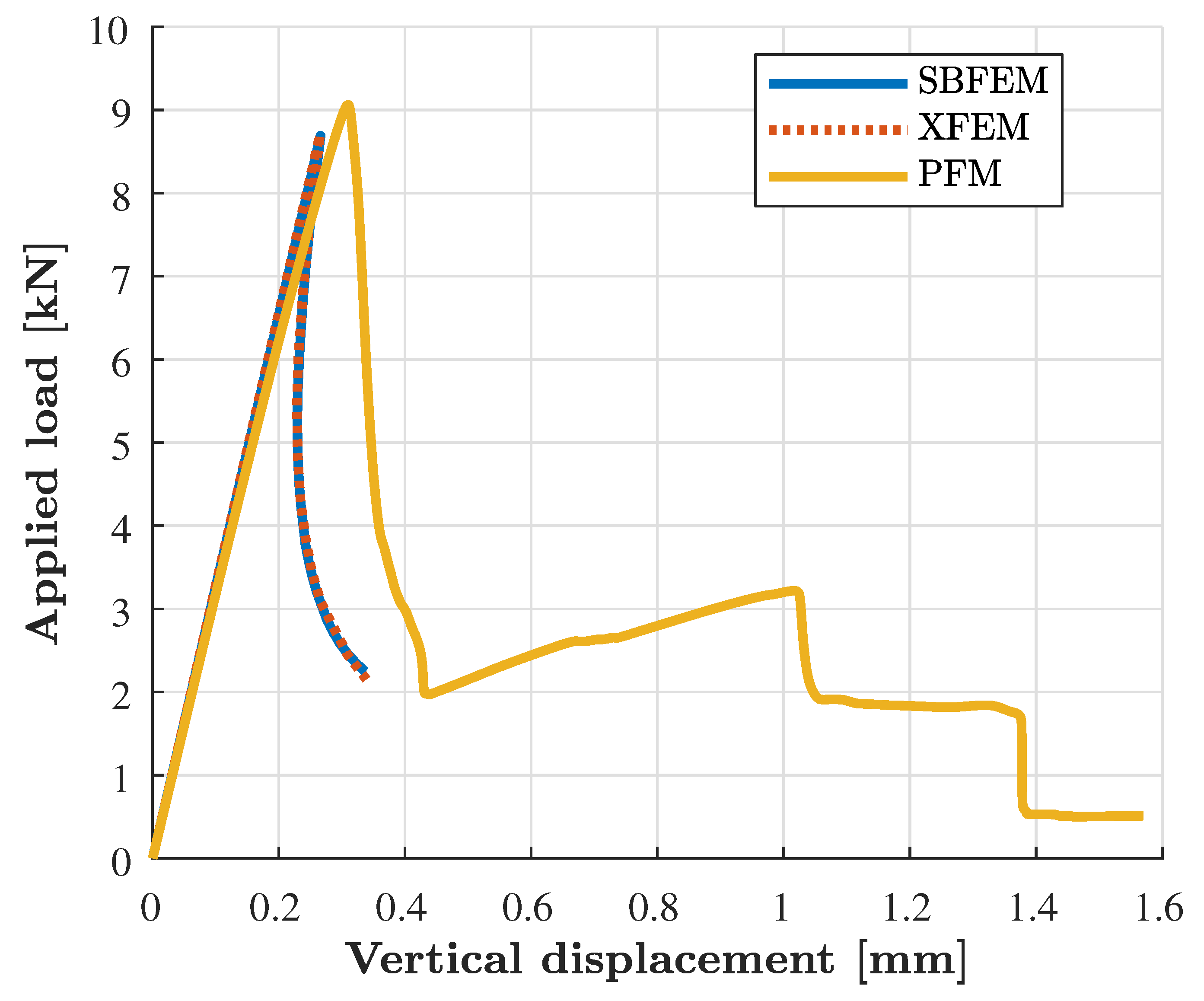
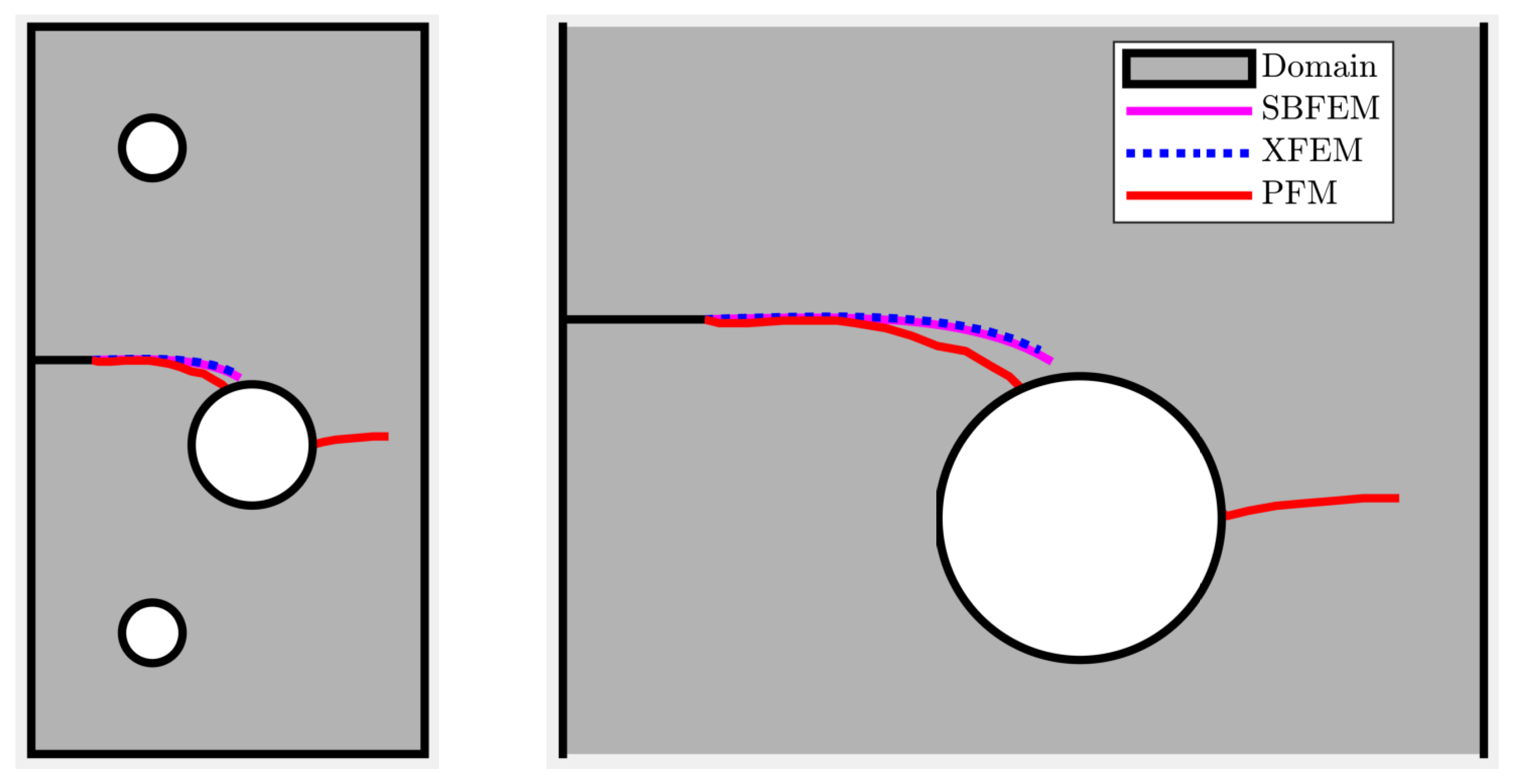
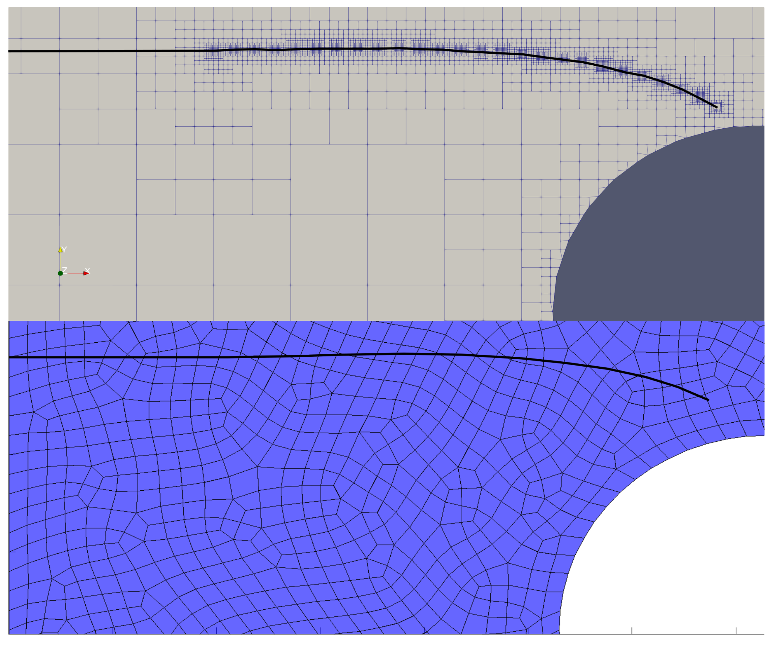
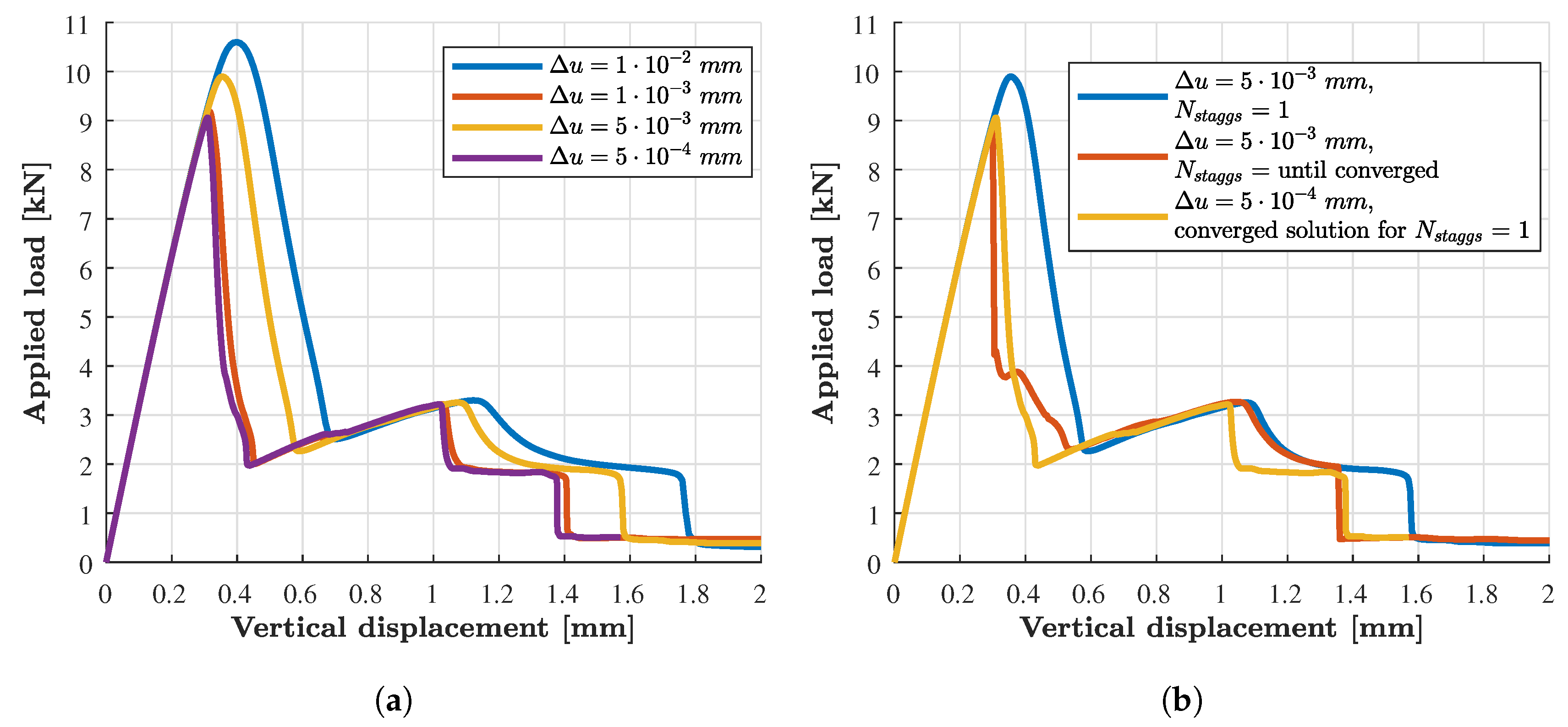
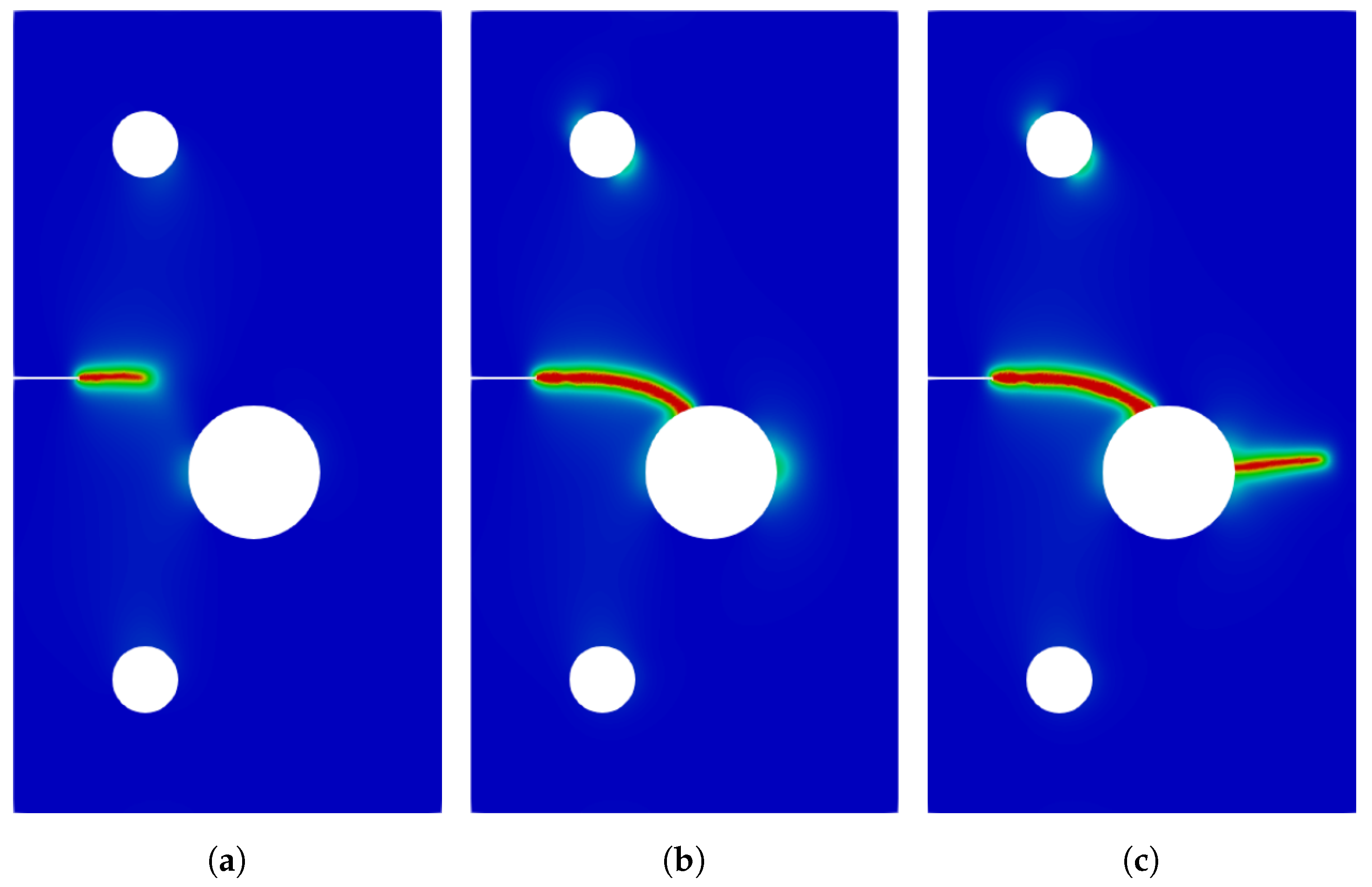
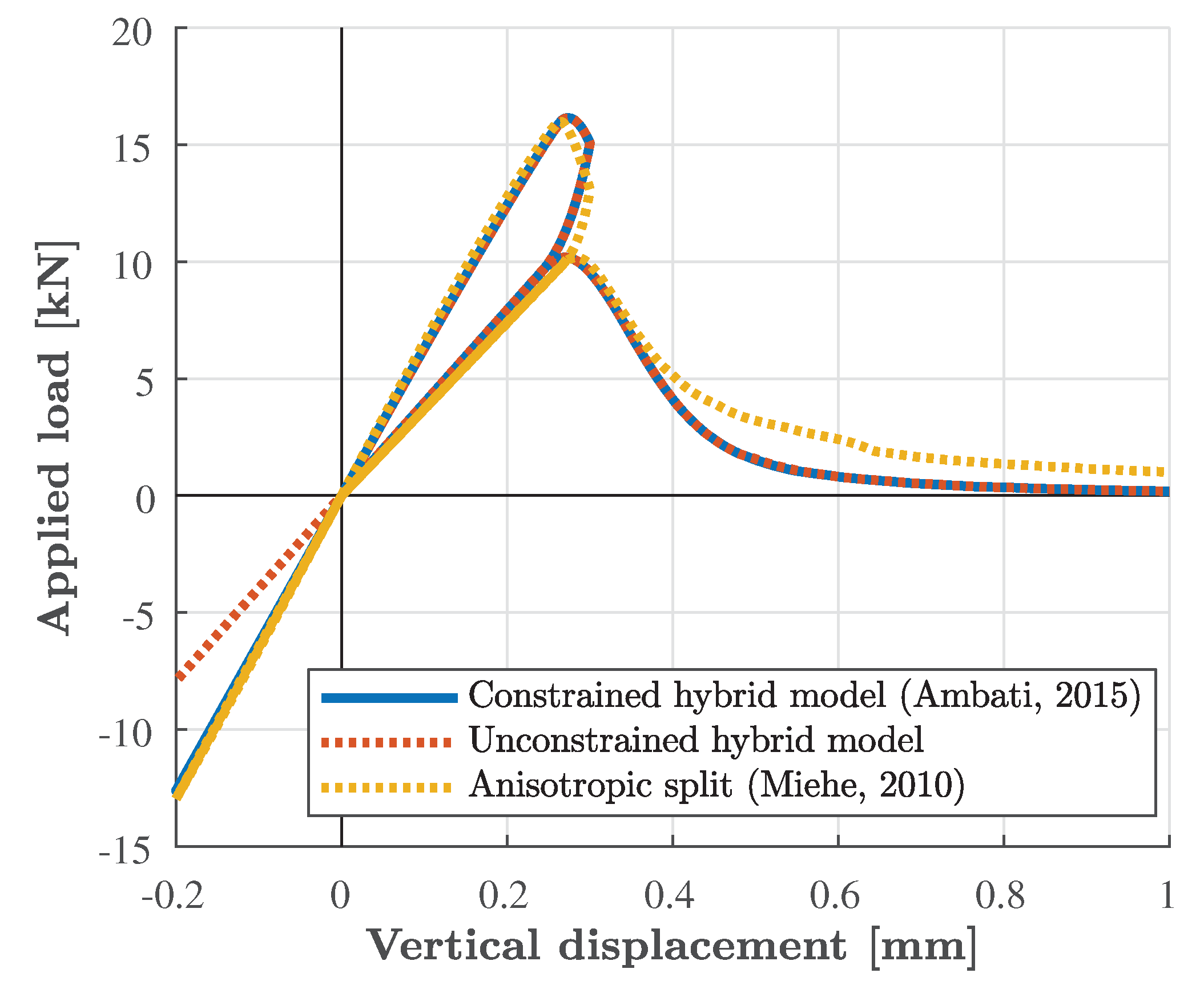
6.6. Numerical Example 5: Plate with Two Holes and Edge Cracks (PwHC)

The case of the plate shown in Figure 37 is considered here. This numerical example is studied, since it poses challenges for both diffuse and discrete methods as discussed in [277]. The boundary conditions and material parameters are also shown in Figure 37 according to [9].
A state of plane strain is considered. The Young’s modulus, Poisson’s ratio, length scale, fracture energy density and crack propagation length are E = 210 kN/mm2, v = 0.3 , l 0 = 0.1  mm, G c = 1.0  N/mm, h P F M 0.06 mm, and  Δ a 1 mm, where applicable. Furthermore, for the phase-field analysis, a volumetric-deviatoric strain decomposition (similar to Amor et al. [264]) is employed. The bottom edge of the plate is clamped, while on the top edge a prescribed displacement is applied in the vertical direction and displacements in the horizontal direction are prohibited ( u x = 0 ; u y > 0 ). The specimen thickness is t = 1  mm.
In the presence of multiple cracks inside a domain, methods employing discrete crack representations typically implement a stability analysis [163] to ascertain the propagating cracks at each step. However, in this specific case, this involved procedure can be circumvented, due to the symmetric test setup. Nevertheless, the naive approach of simply running the analysis will result in an undesirable outcome, since slight numerical imbalances can result in asymmetric and erroneous results. To counteract these effects, symmetric meshes are employed in the XFEM analysis, while the SBFEM analysis enforces symmetric gSIFs about the diagonal. An average of the gSIFs is calculated to determine the crack propagation angle.
Solving this example using the phase-field method produces interesting characteristics with respect to the crack initiation location and crack-paths. It is observed that when there is no restriction imposed on the crack from initiating near the holes, the phase-field initiates simultaneously and symmetrically at the top and bottom hole edges and then propagates almost horizontally as if no notches were present in the structure (Figure 38). However, when the crack evolution is restricted near the hole boundary, e.g., by imposing a very high G c in the surrounding region, the crack initiates at both notch tips and propagates towards the hole edges simultaneously (Figure 39a). Further loading leads to evolution of multiple cracks initiating at the edges of holes which ultimately merge in the centre of the structure (Figure 39d). This observation is similar to what has been previously reported in [277]. However in the absence of experimental results for this problem, it is currently difficult to deduce which method predicts a realistic crack pattern. Hence, we refrain from reporting the typical load-deflection curves and focus only on the crack paths.
Since the crack paths derived from XFEM/SBFEM have been shown to coincide very well when employing similar discretization levels and crack propagation increments, modified mesh discretizations and crack propagation increments are sampled (Figure 40). The crack paths for all three variants align very well for the initial portion, while separating slightly as they approach the holes due to the crack propagation increment and mesh density variations.

7. Discussion and Conclusions

This section initiates by detailing the steps involved in a crack propagation analysis, attempted by each of the described methods. Emphasis is placed on identifying sources of computational effort, while illustrative flowcharts are provided for each method. This visual representation of the methods then serves as a basis for the discussion on the merits and drawbacks of each individual method within the context of LEFM.

7.1. Crack Propagation by XFEM/GFEM

A conceptual representation of the steps involved in a typical crack propagation analysis with the XFEM/GFEM is provided in Figure 41. As should be obvious based on Section 3, enriched finite element methods are essentially discretisation schemes and, as such, require coupling to appropriate criteria in order to model crack propagation. In the present case these are provided by the LEFM framework. The flowchart of Figure 41 involves elastic solution steps followed by the evaluation of a crack propagation criterion. This is common for most LEFM schemes relying on discretizstion, such as for instance FEM or SBFEM. The coupling to further schemes for crack propagation, such as the cohesive zone model, is also possible, in which case the steps of Figure 41 would have to be modified.
The enriched finite element schemes contained within the XFEM/GFEM family of numerical methods permit the treatment of discontinuities and singularities independently of the mesh, while preserving the convergence rates of the underlying FE method. Hence, conventional meshers are employed, yet enriched node and element sets need to be specified and their contributions to the equilibrium equations need to be assembled. This, apart from introducing additional DOFs associated with the enrichment functions (Equation (19)) and potential conditioning problems, requires the use of more involved numerical integration schemes leading to an increased computational toll. Nevertheless, these operations are only performed on a small part of the domain, thus minimizing this additional cost. As mentioned in Section 3, several techniques are available that allow performing the required tasks in a robust and automated manner.
For the calculation of the SIFs, elements within the interaction integral domain are identified and their contributions are assembled. A suitable crack propagation criterion is applied in order to evaluate the propagation direction, and together with a user-specified crack propagation increment Δ a determine the new crack tip location. Since implicit crack representation has become an almost integral part of enriched finite element methods, the next step would involve the update of this representation. This task might introduce additional challenges, however, significant work has been carried out in this direction, with several methods available for tackling this issue in a simplified manner.

7.2. Crack Propagation by SBFEM

The crack propagation process by SBFEM, enhanced via hybrid balanced quadtree polygon meshes, requires the polygon representation of domain features as input, including the crack. The points comprising the polygons constitute the subdivision criterion for the quadtree decomposition. If more than a user-specified number of points fall within a quadrant, this is subdivided. Together with the balancing operation, these steps entail minimal computational effort. The explicit neighbours of each cell do not need to be calculated, but simply the size of its neighbour. This is efficiently achieved by querying the center of each element, offsetting them by the element size in all four cardinal directions, passing them through the tree structure, and finally returning the size of the final cell. Assuming a balanced mesh, all possible element realizations are precomputable. When the domain features, such as the boundary and strong & weak discontinuities do not align with the Cartesian axes, polygon clipping algorithms are required. Although efficient algorithms exist for polygon clipping, the resulting polygonal elements are no longer precomputable and must therefore be calculated individually. In order to construct the stiffness matrix of an SBFEM element, a Hamiltonian eigen-problem must be solved. This entails a real Schur decomposition, sorting of the eigenvalue blocks and subsequent block-diagonalization, as well as the inversion of the matrix [ E 0 ] and the evaluation of a matrix exponential, if quantities of interest inside the SBFEM element need be determined. For smaller elements, commonly employed on quadtree meshes, this additional step when compared to the standard FEM procedure, does not generate a significant computational overhead. Specifically, Ooi et al. [51] report a reduction of computational effort close to 50% on typical analysis domains, when employing precomputable alongside clipped elements. When larger domains are investigated by using a single SBFEM element for the whole domain and hp-refinement is employed, determining the stiffness matrix dominates the computational effort of the analysis. Unfortunately, the stiffness matrix is fully populated, yet symmetric. Hence, this type of analysis is best suited for problems with small boundary to domain ratios. Determining the gSIFs entails post-processing calculations localized to the element containing the crack tip. The singular modes are identified according to Equation (44) and the gSIFs are calculated by evaluating the components of the stress tensor σ ( s ) in crack extension direction (Figure 2b). The crack propagation angle is selected based on a suitable criterion (Equation (13)), while the crack propagation increment Δ a is user specified. After definition of the updated crack tip location, the crack path polyline is updated accordingly and provided as input to the meshing phase of the next iteration. The steps to a standard SBFEM analysis are summarized in Figure 42.

7.3. Crack Propagation by PFM

In PFM fracture is not introduced as an explicit or implicit discontinuity in the displacement field. Rather, it is associated with the evolution of a continuous field, i.e., the phase field. The governing equations of the crack propagation problem emerge through the minimization of the total potential energy established in Equation (70), see, e.g., [69]. This gives rise to the coupled system of equilibrium and phase field governing equations established in Equations (71) and (72). The crack is not explicitly represented but derived from the solution of the coupled system as the region where c = 0 (typically values of c < 10 e 3 ). Within the setting of an incremental solution procedure, the phase field is updated at each time step and with it the crack topology. Nucleation, merging, branching and arrest of cracks as well as the associated crack propagation increment is a natural byproduct of the phase field evolution. The mechanical/phase field coupling is enforced by introducing a material degradation function that is dependent on the phase field. The evolution of fracture follows through the solution of this coupled strong form. Existing discontinuities may be introduced into the domain by providing initial values to the phase field. Mesh density is contingent on sufficient resolution of the fracture process zone, mandating a highly refined mesh in its vicinity. The combination of length scale and level of mesh refinement interact and affect the estimation of the fracture energy hence necessitating the scaling of the critical energy release rate. The numerical solution of the PFM-coupled governing equations is performed using either monolithic or staggered solvers. Monolithic solvers are typically based on the Newton-Raphson solution procedure and have been proven to provide accurate fracture paths. However, they have been shown to suffer from poor convergence due to the non-convex nature of the underlying energy functional [277]. Yet, the accuracy provided by monolithic solvers renders them a favourable solution, especially in the case of dynamic fracture problems and several attempts have been suggested in the literature to improve the robustness of monolithic procedures (see, e.g., [279,280,281]). In staggered methods the displacement and phase field equations are decoupled and solved separately within each load increment. In principle, a staggered algorithm for coupled field problems is based on freezing one field variable at a constant value, solving for the other until convergence is achieved. The staggered approach (also known as alternate minimization approach) provides better convergence rates than the monolithic due to the convexity of the energy functional (Equation (70)) with respect to the two unknown fields { u , ϕ } separately. However, its accuracy is dependent on the incremental step unless stagger iterations are performed; these however increase the computational burden of the analysis. Very recent developments aim towards providing more robust staggered solvers, (see, e.g., [282]). The steps to a typical PFM solution procedure with a staggered solution scheme are summarized in Figure 43.

7.4. Contrasting Discrete and PFM Crack Representation Approaches

The merits of each method within the LEFM setting are discussed by contrasting key features and analysis steps.
For the discrete methods, the representation of the crack is typically available in explicit form. Crack propagation analysis yields a polyline description of the crack topology. Since SBFEM employs polygon clipping, it does not require further information. XFEM, if chosen to employ an implicit enrichment representation, models the crack additionally by associated level sets. Crack path extraction is not necessary, since it is already given as a polyline. A crack consisting of a one-segment polyline is usually provided as input. For the PFM, the crack is represented by a scalar phase-field, with the phase-field variable directly embedded into the constitutive equations. The crack is represented as the region of fully degraded material with c = 0 . Hence, no explicit crack representation is required during the analysis, albeit readily available in post-processing, if required. Initial defects are introduced in the system by specifying sets of points with corresponding phase field values.
Meshing requirements for analysis by XFEM are largely decoupled due to the level set representation, yet substituted by more involved numerical integration procedures. This permits the use of a constant mesh during crack propagation analysis. This is contrary to analysis by SBFEM, where the initial quadtree decomposition, i.e., the mesh, is updated during each step incrementally. Discontinuities introduced by polygon clipping result in double nodes, such that the nDOF of the system increase gradually as the analysis proceeds. Furthermore, in select cases, clipping can result in non star-convex elements, which the method cannot treat. Delaunay triangulation of the element is required in such instances. Furthermore, due to clipping, elements with poor aspect ratios, in the conventional FEM sense, may arise. Empirically, this does not seem to be as severe an issue manifesting itself in erroneous numerical integration results, when employing SBFEM. In order to adequately represent the fracture process zone, the PFM requires a highly refined mesh in the regions of expected crack propagation as well as at the crack tip, rendering the phase-field method computationally expensive for solving large-scale problems, especially when compared to discrete fracture approaches. It is now accepted that an element size h l 0 is required to accurately resolve the crack path. However, this computational burden is effectively addressed using parallel solvers, adaptive mesh refinement [229,283], multiscale computation techniques [284] also within a local/global solution context [285].
The methods further differ in the hyper-parameters that ought to be specified by the analyst. XFEM requires the specification of crack tip enrichment type and radius, as well as the region where the interaction integral is to be calculated. Special care must be taken to exclude blending elements from the calculation of the SIFs, which may affect final results. SBFEM similarly requires the analyst to specify the homogenization region about the crack tip. With the exception of the cohesive phase field model, in the PFM implementations discussed in Section 5.2 the specification of the length scale regulates the response, imposing guidelines on mesh discretization and scaling of the critical fracture energy. As further discussed in Section 5.2, early efforts to treat this regulatory effect by introducing stress-based crack-driving forces have been reported in [256] whereas, and most notably, Wu and Nguyen [251] provided length-scale insensitive formulations that also preserve Γ -convergence.
The solution process for both XFEM and SBFEM involves a single elastic solution step. The PFM, as previously described in Section 7.3, comprises either monolithic or staggered approaches within an iterative solution scheme. In the quasi-static regime, displacement or generalised control solution procedures are typically employed. This however necessitates that either Equations (71) and (72) must be solved with very small time-increments (typically 10 5 10 6 ), or stagger iterations must be performed between both equations to ensure energy convergence. Often both of these options lead to high computational cost.
Therefore, the corresponding load-deflection curve follows from the solution at every time step. In such quasi-static analyses, displacement controlled analysis automatically yields the load-deflection curve along with the softening branch. The discrete crack methods derive the load deflection curve in back-calculation. To this end, an arbitrary loading, e.g., force- or displacement-based, is applied. The resulting equivalent SIF is compared to the critical stress intensity factor. Hence, a scaling factor is derived for the loads and displacements at which crack propagation is initiated. This implies that recovery of the linear branch is a one-step process. Recovering an explicit linear elastic branch with the PFM requires either a linear phase field approximation as in Section 5.2.3 or cubic degradation functions [80]. Absence of these approaches will yield deviations from the linear elastic behaviour contingent on the evolution of material degradation in the process zone. Since the overall system stiffness is underestimated, the associated displacements are overestimated accordingly.
In the PFM a crack is never explicitly propagated, but associated with the evolution of the phase field that emerges from the solution of the phase field governing equation. This is driven by the definition of the crack driving force as discussed in Section 5.2. Depending on the PFM formulation employed, the crack driving force can be established on the basis of either energy or limit-stress criteria. The discrete crack methods, within the LEFM framework, require the calculation of the crack propagation angle and some crack propagation increment. Examples of the later are either user specified or provided by Paris’ equation. The crack is assumed to propagate in a straight line, originating from the crack tip determined in the previous analysis step. Hence, the history variables required are none other than the polyline for SBFEM, while XFEM propagates the associated level sets as well. PFM require updating the scalar phase field and specific realization of the PFM require further history variables to impose the crack-irreversibility condition, preventing the crack from healing during cyclic loading.
The fact that the solution of the phase field governing equations emerge from an energy minimization problem, opposite to discrete fracture approaches, enables the resolution of crack initiation without the requirement for a crack path to be defined a priori. Furthermore, crack nucleation, growth and coalescence happen automatically; this results in a robust method with enormous flexibility to model complex cracking patterns including the simulation of curvillinear cracks, crack merging, and crack branching without the need for ad-hoc crack tracking methods. Finally, the method is naturally extended to 3D [229], considering also the case of fracture under multi-physics scenaria, e.g., temperature induced fracture [256,286], hydraulic fracturing [81,82,84,287,288], and diffusion [289]. These advantages, render the phase-field approach a robust crack prediction method. Compared to discrete fracture approaches, the variational structure upon which the phase field theory emerges, equips it with significant capabilities for modelling diverse and complex fracture problems in a unified and consistent manner.
The major advantage of the diffuse crack methods and the PFM specifically lies in their generality. Extending the discrete crack methods to exhibit similar capabilities involves significant algorithmic changes, as these codes are custom and not readily extendable to further types of analysis. Furthermore, extension to 3D problems is not straightforward, in addition, the definition of crack propagation increment in 3D is difficult to specify. Furthermore, judging if a crack arrests or the method simply does not permit continuation across obstacles, requires expert knowledge.

Author Contributions

The idea for this review emerged from discussions held between E.C. and S.P.T.; A.E. was responsible for the SBFEM source code implementation and simulations, the discussion on the merits and drawbacks of the examined methods, and the consistent presentation of the results; K.A. was responsible for the XFEM source code implementation and simulations; U.P., E.K., and S.P.T. were responsible for the phase field source code implementation and simulations. E.C., S.P.T., and I.A.A., advised on the simulation methods, the manuscript organization, and contributed in the discussion of the results. The first three authors contributed equally to paper writing.

Funding

This research was performed under the auspices of the Swiss National Science Foundation (SNSF), Grant # 200021_153379, A Multiscale Hysteretic XFEM Scheme for the Analysis of Composite Structures. Konstantinos Agathos would like to acknowledge funding received from the European Union’s Horizon 2020 research and innovation programme under the Marie Sklodowska-Curie grant agreement No. 795917 “SiMAero, Simulation-Driven and On-line Condition Monitoring with Applications to Aerospace”. Udit Pillai, Savvas Triantafyllou, and Ian Aschroft would like to acknowledge funding received from the European Union’s Horizon 2020 research and innovation programme under the Marie Skłodowska-Curie SAFE-FLY project, grant agreement No. 721455.

Acknowledgments

The authors are grateful to the University of Nottingham for access to its High Performance Computing facility and extend their gratitude to the group of Song from UNSW and in particular Albert Saputra for his guidance on SBFEM implementation.

Conflicts of Interest

The authors declare no conflict of interest. The funders had no role in the design of the study; in the collection, analyses, or interpretation of data; in the writing of the manuscript, or in the decision to publish the results.

References

  1. Zheng, J.; Liu, P. Elasto-plastic stress analysis and burst strength evaluation of Al-carbon fiber/epoxy composite cylindrical laminates. Comput. Mater. Sci. 2008, 42, 453–461. [Google Scholar] [CrossRef]
  2. Xu, P.; Zheng, J.; Liu, P. Finite element analysis of burst pressure of composite hydrogen storage vessels. Mater. Des. 2009, 30, 2295–2301. [Google Scholar] [CrossRef]
  3. Liu, P.; Zheng, J. Recent developments on damage modeling and finite element analysis for composite laminates: A review. Mater. Des. 2010, 31, 3825–3834. [Google Scholar] [CrossRef]
  4. Ravi-Chandar, K.; Knauss, W. An experimental investigation into dynamic fracture: III. On steady-state crack propagation and crack branching. Int. J. Fract. 1984, 26, 141–154. [Google Scholar] [CrossRef]
  5. Ravi-Chandar, K. Dynamic fracture of nominally brittle materials. Int. J. Fract. 1998, 90, 83–102. [Google Scholar] [CrossRef]
  6. Anderson, T.L. Fracture Mechanics: Fundamentals and Applications; CRC Press: Boca Raton, FL, USA, 2017. [Google Scholar]
  7. Murakami, S. Continuum Damage Mechanics: A Continuum Mechanics Approach to the Analysis of Damage and Fracture; Springer Science & Business Media: Berlin, Germany, 2012; Volume 185. [Google Scholar]
  8. Bittencourt, T.; Wawrzynek, P.; Ingraffea, A.; Sousa, J. Quasi-automatic simulation of crack propagation for 2D LEFM problems. Eng. Fract. Mech. 1996, 55, 321–334. [Google Scholar] [CrossRef]
  9. Bouchard, P.; Bay, F.; Chastel, Y. Numerical modelling of crack propagation: Automatic remeshing and comparison of different criteria. Comput. Methods Appl. Mech. Eng. 2003, 192, 3887–3908. [Google Scholar] [CrossRef]
  10. Azócar, D.; Elgueta, M.; Rivara, M.C. Automatic LEFM crack propagation method based on local Lepp–Delaunay mesh refinement. Adv. Eng. Softw. 2010, 41, 111–119. [Google Scholar] [CrossRef]
  11. Kirk, B.S.; Peterson, J.W.; Stogner, R.H.; Carey, G.F. libMesh: A C++ library for parallel adaptive mesh refinement/coarsening simulations. Eng. Comput. 2006, 22, 237–254. [Google Scholar] [CrossRef]
  12. Geuzaine, C.; Remacle, J.F. Gmsh: A 3-D finite element mesh generator with built-in pre- and post-processing facilities. Int. J. Numer. Methods Eng. 2009, 79, 1309–1331. [Google Scholar] [CrossRef]
  13. Barsoum, R. On the use of isoparametric finite elements in linear fracture mechanics. Int. J. Numer. Methods Eng. 1976, 10, 25–37. [Google Scholar] [CrossRef]
  14. Moran, B.; Shih, C. Crack tip and associated domain integrals from momentum and energy balance. Eng. Fract. Mech. 1987, 27, 615–642. [Google Scholar] [CrossRef]
  15. Gosz, M.; Moran, B. An interaction energy integral method for computation of mixed-mode stress intensity factors along non-planar crack fronts in three dimensions. Eng. Fract. Mech. 2002, 69, 299–319. [Google Scholar] [CrossRef]
  16. Courtin, S.; Gardin, C.; Bézine, G.; Ben Hadj Hamouda, H. Advantages of the J-integral approach for calculating stress intensity factors when using the commercial finite element software ABAQUS. Eng. Fract. Mech. 2005, 72, 2174–2185. [Google Scholar] [CrossRef]
  17. Kim, J.H.; Paulino, G.H. The interaction integral for fracture of orthotropic functionally graded materials: Evaluation of stress intensity factors. Int. J. Solids Struct. 2003, 40, 3967–4001. [Google Scholar] [CrossRef]
  18. Rybicki, E.; Kanninen, M. A finite element calculation of stress intensity factors by a modified crack closure integral. Eng. Fract. Mech. 1977, 9, 931–938. [Google Scholar] [CrossRef]
  19. Raju, I. Calculation of strain-energy release rates with higher order and singular finite elements. Eng. Fract. Mech. 1987, 28, 251–274. [Google Scholar] [CrossRef]
  20. Krueger, R. Virtual crack closure technique: History, approach, and applications. Appl. Mech. Rev. 2004, 57, 109. [Google Scholar] [CrossRef]
  21. Karihaloo, B.; Xiao, Q. Accurate determination of the coefficients of elastic crack tip asymptotic field by a hybrid crack element with p-adaptivity. Eng. Fract. Mech. 2001, 68, 1609–1630. [Google Scholar] [CrossRef]
  22. Karihaloo, B.L.; Xiao, Q.Z. Asymptotic fields at the tip of a cohesive crack. Int. J. Fract. 2008, 150, 55–74. [Google Scholar] [CrossRef]
  23. Wang, Y.; Cerigato, C.; Waisman, H.; Benvenuti, E. XFEM with high-order material-dependent enrichment functions for stress intensity factors calculation of interface cracks using Irwin’s crack closure integral. Eng. Fract. Mech. 2017, 178, 148–168. [Google Scholar] [CrossRef]
  24. Belytschko, T.; Lu, Y.; Gu, L. Element-free Galerkin methods. Int. J. Numer. Methods Eng. 1994, 37, 229–256. [Google Scholar] [CrossRef]
  25. Belytschko, T.; Gu, L.; Lu, Y. Fracture and crack growth by element free Galerkin methods. Model. Simul. Mater. Sci. Eng. 1994, 2, 519. [Google Scholar] [CrossRef]
  26. Lu, Y.; Belytschko, T.; Gu, L. A new implementation of the element free Galerkin method. Comput. Methods Appl. Mech. Eng. 1994, 113, 397–414. [Google Scholar] [CrossRef]
  27. Nguyen, V.P.; Rabczuk, T.; Bordas, S.; Duflot, M. Meshless methods: A review and computer implementation aspects. Math. Comput. Simul. 2008, 79, 763–813. [Google Scholar] [CrossRef] [Green Version]
  28. Sulsky, D.; Chen, Z.; Schreyer, H.L. A particle method for history-dependent materials. Comput. Methods Appl. Mech. Eng. 1994, 118, 179–196. [Google Scholar] [CrossRef]
  29. Cottet, G.H.; Raviart, P.A. On particle-in-cell methods for the Vlasov-Poisson equations. Transp. Theory Stat. Phys. 1986, 15, 1–31. [Google Scholar] [CrossRef]
  30. Nairn, J.A. Material point method calculations with explicit cracks. Comput. Model. Eng. Sci. 2003, 4, 649–664. [Google Scholar]
  31. Moutsanidis, G.; Kamensky, D.; Zhang, D.Z.; Bazilevs, Y.; Long, C.C. Modeling strong discontinuities in the material point method using a single velocity field. Comput. Methods Appl. Mech. Eng. 2019, 345, 584–601. [Google Scholar] [CrossRef]
  32. Kakouris, E.; Triantafyllou, S.P. Phase-field material point method for brittle fracture. Int. J. Numer. Methods Eng. 2017, 112, 1750–1776. [Google Scholar] [CrossRef]
  33. Kakouris, E.; Triantafyllou, S. Material point method for crack propagation in anisotropic media: A phase field approach. Arch. Appl. Mech. 2018, 88, 287–316. [Google Scholar] [CrossRef]
  34. Maschke, H.G.; Kuna, M. A review of boundary and finite element methods in fracture mechanics. Theor. Appl. Fract. Mech. 1985, 4, 181–189. [Google Scholar] [CrossRef]
  35. Rokhlin, V. Rapid solution of integral equations of classical potential theory. J. Comput. Phys. 1985, 60, 187–207. [Google Scholar] [CrossRef]
  36. Hackbusch, W. A Sparse Matrix Arithmetic Based on $\Cal H$-Matrices. Part I: Introduction to ${\Cal H}$-Matrices. Computing 1999, 62, 89–108. [Google Scholar] [CrossRef]
  37. Hughes, T.; Cottrell, J.; Bazilevs, Y. Isogeometric analysis: CAD, finite elements, NURBS, exact geometry and mesh refinement. Comput. Methods Appl. Mech. Eng. 2005, 194, 4135–4195. [Google Scholar] [CrossRef] [Green Version]
  38. Nguyen, V.P.; Anitescu, C.; Bordas, S.P.; Rabczuk, T. Isogeometric analysis: An overview and computer implementation aspects. Math. Comput. Simul. 2015, 117, 89–116. [Google Scholar] [CrossRef] [Green Version]
  39. Li, K.; Qian, X. Isogeometric analysis and shape optimization via boundary integral. Comput.-Aided Des. 2011, 43, 1427–1437. [Google Scholar] [CrossRef]
  40. Simpson, R.N.; Bordas, S.; Trevelyan, J.; Rabczuk, T. A two-dimensional isogeometric boundary element method for elastostatic analysis. Comput. Methods Appl. Mech. Eng. 2012, 209, 87–100. [Google Scholar] [CrossRef]
  41. Scott, M.; Simpson, R.; Evans, J.; Lipton, S.; Bordas, S.; Hughes, T.; Sederberg, T. Isogeometric boundary element analysis using unstructured T-splines. Comput. Methods Appl. Mech. Eng. 2013, 254, 197–221. [Google Scholar] [CrossRef]
  42. Nguyen, T.T.; Yvonnet, J.; Zhu, Q.Z.; Bornert, M.; Chateau, C. A phase-field method for computational modeling of interfacial damage interacting with crack propagation in realistic microstructures obtained by microtomography. Comput. Methods Appl. Mech. Eng. 2016, 312, 567–595. [Google Scholar] [CrossRef] [Green Version]
  43. Peng, X.; Atroshchenko, E.; Kerfriden, P.; Bordas, S. Isogeometric boundary element methods for three dimensional static fracture and fatigue crack growth. Comput. Methods Appl. Mech. Eng. 2017, 316, 151–185. [Google Scholar] [CrossRef]
  44. Moës, N.; Dolbow, J.; Belytschko, T. A finite element method for crack growth without remeshing. Int. J. Numer. Methods Eng. 1999, 46, 131–150. [Google Scholar] [CrossRef]
  45. Strouboulis, T.; Babuška, I.; Copps, K. The design and analysis of the generalized finite element method. Comput. Methods Appl. Mech. Eng. 2000, 181, 43–69. [Google Scholar] [CrossRef]
  46. Babuška, I.; Caloz, G.; Osborn, J. Special finite element methods for a class of second order elliptic problems with rough coefficients. SIAM J. Numer. Anal. 1994, 31, 945–981. [Google Scholar] [CrossRef]
  47. Babuška, I.; Melenk, J. The partition of unity method. Int. J. Numer. Methods Eng. 1996, 40, 727–758. [Google Scholar] [CrossRef]
  48. Melenk, J.; Babuška, I. The partition of unity finite element method: Basic theory and applications. Comput. Methods Appl. Mech. Eng. 1996, 139, 289–314. [Google Scholar] [CrossRef] [Green Version]
  49. Wolf, J.P.; Song, C. Consistent infinitesimal finite-element cell method: In-plane motion. Comput. Methods Appl. Mech. Eng. 1995, 123, 355–370. [Google Scholar] [CrossRef]
  50. Song, C.; Tin-Loi, F.; Gao, W. A definition and evaluation procedure of generalized stress intensity factors at cracks and multi-material wedges. Eng. Fract. Mech. 2010, 77, 2316–2336. [Google Scholar] [CrossRef]
  51. Ooi, E.; Man, H.; Natarajan, S.; Song, C. Adaptation of quadtree meshes in the scaled boundary finite element method for crack propagation modelling. Eng. Fract. Mech. 2015, 144, 101–117. [Google Scholar] [CrossRef] [Green Version]
  52. Barenblatt, G.I. The Mathematical Theory of Equilibrium Cracks in Brittle Fracture. Adv. Appl. Mech. 1962, 7, 55–129. [Google Scholar]
  53. Dugdale, D.S. Yielding of Steel Sheets Containing Slits. J. Mech. Phys. Solids 1960, 8, 100–104. [Google Scholar] [CrossRef]
  54. Xu, X.P.; Needleman, A. Numerical simulations of fast crack growth in brittle solids. J. Mech. Phys. Solids 1994, 42, 1397–1434. [Google Scholar] [CrossRef]
  55. Chen, Z.; Bunger, A.P.; Zhang, X.; Jeffrey, R.G. Cohesive zone finite element-based modeling of hydraulic fractures. Acta Mech. Solida Sin. 2009, 22, 443–452. [Google Scholar] [CrossRef]
  56. Salen, A.L.; Aliabadi, M.H. Crack growth analysis in concrete using boundary element method. Eng. Fract. Mech. 1995, 51, 533–545. [Google Scholar]
  57. Nguyen, T.C.; Bui, H.H.; Nguyen, P.V.; Nguyen, G.D. A Conceptual Approach to Modelling Rock Fracture using the Smoothed Particle Hydrodynamics and Cohesive Cracks. In Proceedings of the ISRM Regional Symposium-EUROCK 2015, Salzburg, Austria, 7–10 October 2015; International Society for Rock Mechanics and Rock Engineering: Lisbon, Portugal, 2015. [Google Scholar]
  58. Klein, P.A.; Foulk, J.W.; Chen, E.P.; Wimmer, S.A.; Gao, H.J. Physics-based modeling of brittle fracture: Cohesive formulations and the application of meshfree methods. Theor. Appl. Fract. Mech. 2001, 37, 99–166. [Google Scholar] [CrossRef]
  59. Soparat, P.; Nanakorn, P. Analysis of Cohesive Crack Growth by the Element-Free Galerkin Method. J. Mech. 2008, 24, 45–54. [Google Scholar] [CrossRef] [Green Version]
  60. Remmers, J.J.C.; de Borst, R.; Needleman, A. A cohesive segments method for the simulation of crack growth. Comput. Mech. 2003, 31, 69–77. [Google Scholar] [CrossRef] [Green Version]
  61. Remmers, J.J.C.; de Borst, R.; Needleman, A. The simulation of dynamic crack propagation using the cohesive segments method. J. Mech. Phys. Solids 2008, 56, 70–92. [Google Scholar] [CrossRef]
  62. Rabczuk, T.; Zi, G. A Meshfree Method based on the Local Partition of Unity for Cohesive Cracks. Comput. Mech. 2007, 39, 743–760. [Google Scholar] [CrossRef]
  63. Barbieri, E.; Meo, M. A Meshless Cohesive Segments Method for Crack Initiation and Propagation in Composites. Appl. Compos. Mater. 2011, 18, 45–63. [Google Scholar] [CrossRef]
  64. Msekh, M.A.; Sargado, J.M.; Jamshidian, M.; Areias, P.M.; Rabczuk, T. Abaqus implementation of phase-field model for brittle fracture. Comput. Mater. Sci. 2015, 96, 472–484. [Google Scholar] [CrossRef]
  65. Rashid, Y. Ultimate strength analysis of prestressed concrete pressure vessels. Nucl. Eng. Des. 1968, 7, 334–344. [Google Scholar] [CrossRef]
  66. Peerlings, R.D.; De Borst, R.; Brekelmans, W.D.; De Vree, J. Gradient enhanced damage for quasi-brittle materials. Int. J. Numer. Methods Eng. 1996, 39, 3391–3403. [Google Scholar] [CrossRef]
  67. Simone, A.; Wells, G.N.; Sluys, L.J. From continuous to discontinuous failure in a gradient-enhanced continuum damage model. Comput. Methods Appl. Mech. Eng. 2003, 192, 4581–4607. [Google Scholar] [CrossRef]
  68. Moës, N.; Stolz, C.; Bernard, P.E.; Chevaugeon, N. A level set based model for damage growth: The thick level set approach. Int. J. Numer. Methods Eng. 2011, 86, 358–380. [Google Scholar] [CrossRef]
  69. Bourdin, B.; Francfort, G.A.; Marigo, J.J. The variational approach to fracture. J. Elast. 2008, 91, 5–148. [Google Scholar] [CrossRef]
  70. De Borst, R.; Verhoosel, C.V. Gradient damage vs phase-field approaches for fracture: Similarities and differences. Comput. Methods Appl. Mech. Eng. 2016, 312, 78–94. [Google Scholar] [CrossRef] [Green Version]
  71. Mandal, T.K.; Nguyen, V.P.; Heidarpour, A. Phase field and gradient enhanced damage models for quasi-brittle failure: A numerical comparative study. Eng. Fract. Mech. 2019, 207, 48–67. [Google Scholar] [CrossRef]
  72. Cazes, F.; Moës, N. Comparison of a phase-field model and of a thick level set model for brittle and quasi-brittle fracture. Int. J. Numer. Methods Eng. 2015, 103, 114–143. [Google Scholar] [CrossRef]
  73. Francfort, G.A.; Marigo, J.J. Revisiting brittle fracture as an energy minimization problem. J. Mech. Phys. Solids 1998, 46, 1319–1342. [Google Scholar] [CrossRef]
  74. Ambrosio, L.; Tortorelli, V.M. Approximation of functional depending on jumps by elliptic functional via Γ-convergence. Commun. Pure Appl. Math. 1990, 43, 999–1036. [Google Scholar] [CrossRef]
  75. Aldakheel, F.; Hudobivnik, B.; Hussein, A.; Wriggers, P. Phase-field modeling of brittle fracture using an efficient virtual element scheme. Comput. Methods Appl. Mech. Eng. 2018, 341, 443–466. [Google Scholar] [CrossRef]
  76. Moutsanidis, G.; Kamensky, D.; Chen, J.; Bazilevs, Y. Hyperbolic phase field modeling of brittle fracture: Part II-immersed IGA-RKPM coupling for air-blast-structure interaction. J. Mech. Phys. Solids 2018, 121, 114–132. [Google Scholar] [CrossRef]
  77. Alessi, R.; Vidoli, S.; De Lorenzis, L. A phenomenological approach to fatigue with a variational phase-field model: The one-dimensional case. Eng. Fract. Mech. 2018, 190, 53–73. [Google Scholar] [CrossRef]
  78. Wu, J.; Wang, D.; Lin, Z.; Qi, D. An efficient gradient smoothing meshfree formulation for the fourth-order phase field modeling of brittle fracture. Comput. Part. Mech. 2019. [Google Scholar] [CrossRef]
  79. Ambati, M.; Kruse, R.; De Lorenzis, L. A phase-field model for ductile fracture at finite strains and its experimental verification. Comput. Mech. 2016, 57, 149–167. [Google Scholar] [CrossRef]
  80. Borden, M.J.; Hughes, T.J.; Landis, C.M.; Anvari, A.; Lee, I.J. A phase-field formulation for fracture in ductile materials: Finite deformation balance law derivation, plastic degradation, and stress triaxiality effects. Comput. Methods Appl. Mech. Eng. 2016, 312, 130–166. [Google Scholar] [CrossRef] [Green Version]
  81. Wilson, Z.A.; Landis, C.M. Phase-field modeling of hydraulic fracture. J. Mech. Phys. Solids 2016, 96, 264–290. [Google Scholar] [CrossRef] [Green Version]
  82. Miehe, C.; Mauthe, S. Phase field modeling of fracture in multi-physics problems. Part III. Crack driving forces in hydro-poro-elasticity and hydraulic fracturing of fluid-saturated porous media. Comput. Methods Appl. Mech. Eng. 2016, 304, 619–655. [Google Scholar] [CrossRef]
  83. Heider, Y.; Markert, B. A phase-field modeling approach of hydraulic fracture in saturated porous media. Mech. Res. Commun. 2017, 80, 38–46. [Google Scholar] [CrossRef]
  84. Ehlers, W.; Luo, C. A phase-field approach embedded in the Theory of Porous Media for the description of dynamic hydraulic fracturing. Comput. Methods Appl. Mech. Eng. 2017, 315, 348–368. [Google Scholar] [CrossRef]
  85. Pillai, U.; Heider, Y.; Markert, B. A diffusive dynamic brittle fracture model for heterogeneous solids and porous materials with implementation using a user-element subroutine. Comput. Mater. Sci. 2018, 153, 36–47. [Google Scholar] [CrossRef]
  86. Griffith, A. The phenomena of rupture and flow in solids. Philos. Trans. R. Soc. Lond. Ser. A Contain. Pap. Math. Phys. Character 1920, 221, 163–198. [Google Scholar] [CrossRef]
  87. Erdogan, F.; Sih, G. On the crack extension in plates under plane loading and transverse shear. J. Basic Eng. 1963, 85, 519–525. [Google Scholar] [CrossRef]
  88. Nuismer, R. An energy release rate criterion for mixed mode fracture. Int. J. Fract. 1975, 11, 245–250. [Google Scholar] [CrossRef]
  89. Sih, G. Strain-energy-density factor applied to mixed mode crack problems. Int. J. Fract. 1974, 10, 305–321. [Google Scholar] [CrossRef]
  90. Abdelaziz, Y.; Hamouine, A. A survey of the extended finite element. Comput. Struct. 2008, 86, 1141–1151. [Google Scholar] [CrossRef]
  91. Belytschko, T.; Gracie, R.; Ventura, G. A review of extended/generalized finite element methods for material modeling. Model. Simul. Mater. Sci. Eng. 2009, 17, 043001. [Google Scholar] [CrossRef]
  92. Fries, T.; Belytschko, T. The extended/generalized finite element method: An overview of the method and its applications. Int. J. Numer. Methods Eng. 2010, 84, 253–304. [Google Scholar] [CrossRef]
  93. Sukumar, N.; Dolbow, J.; Moës, N. Extended finite element method in computational fracture mechanics: A retrospective examination. Int. J. Fract. 2015, 196, 189–206. [Google Scholar] [CrossRef]
  94. Zhang, Q.; Banerjee, U.; Babuška, I. Higher order stable generalized finite element method. Numer. Math. 2014, 128, 1–29. [Google Scholar] [CrossRef]
  95. Griebel, M.; Schweitzer, M. A particle-partition of unity method part VII: Adaptivity. In Meshfree Methods for Partial Differential Equations III; Springer: Berlin, Germany, 2007; pp. 121–147. [Google Scholar]
  96. Hong, W.; Lee, P. Mesh based construction of flat-top partition of unity functions. Appl. Math. Comput. 2013, 219, 8687–8704. [Google Scholar] [CrossRef]
  97. Belytschko, T.; Black, T. Elastic crack growth in finite elements with minimal remeshing. Int. J. Numer. Methods Eng. 1999, 620, 601–620. [Google Scholar] [CrossRef]
  98. Hansbo, A.; Hansbo, P. A finite element method for the simulation of strong and weak discontinuities in solid mechanics. Comput. Methods Appl. Mech. Eng. 2004, 193, 3523–3540. [Google Scholar] [CrossRef]
  99. Mariani, S.; Perego, U. Extended finite element method for quasi-brittle fracture. Int. J. Numer. Methods Eng. 2003, 58, 103–126. [Google Scholar] [CrossRef]
  100. Cheng, K.; Fries, T. Higher-order XFEM for curved strong and weak discontinuities. Int. J. Numer. Methods Eng. 2010, 82, 564–590. [Google Scholar] [CrossRef]
  101. Agathos, K.; Chatzi, E.; Bordas, S. A unified enrichment approach addressing blending and conditioning issues in enriched finite elements. Comput. Methods Appl. Mech. Eng. 2019, 349, 673–700. [Google Scholar] [CrossRef]
  102. Duarte, C.; Reno, L.; Simone, A. A high-order generalized FEM for through-the-thickness branched cracks. Int. J. Numer. Methods Eng. 2007, 72, 325–351. [Google Scholar] [CrossRef]
  103. Daux, C.; Moës, N.; Dolbow, J.; Sukumar, N.; Belytschko, T. Arbitrary branched and intersecting cracks with the extended finite element method. Int. J. Numer. Methods Eng. 2000, 48, 1741–1760. [Google Scholar] [CrossRef]
  104. Stazi, F.; Budyn, E.; Chessa, J.; Belytschko, T. An extended finite element method with higher-order elements for curved cracks. Comput. Mech. 2003, 31, 38–48. [Google Scholar] [CrossRef]
  105. Laborde, P.; Pommier, J.; Renard, Y.; Salaün, M. High-order extended finite element method for cracked domains. Int. J. Numer. Methods Eng. 2005, 64, 354–381. [Google Scholar] [CrossRef] [Green Version]
  106. Béchet, E.; Minnebo, H.; Moës, N.; Burgardt, B. Improved implementation and robustness study of the X-FEM for stress analysis around cracks. Int. J. Numer. Methods Eng. 2005, 64, 1033–1056. [Google Scholar] [CrossRef] [Green Version]
  107. Duarte, C.; Babuška, I.; Oden, J. Generalized finite element methods for three-dimensional structural mechanics problems. Comput. Struct. 2000, 77, 215–232. [Google Scholar] [CrossRef] [Green Version]
  108. Xiao, Q.; Karihaloo, B. Direct evaluation of accurate coefficients of the linear elastic crack tip asymptotic field. Fatigue Fract. Eng. Mater. Struct. 2003, 26, 719–729. [Google Scholar] [CrossRef]
  109. Liu, X.; Xiao, Q.; Karihaloo, B. XFEM for direct evaluation of mixed mode SIFs in homogeneous and bi-materials. Int. J. Numer. Methods Eng. 2004, 59, 1103–1118. [Google Scholar] [CrossRef]
  110. Zamani, A.; Gracie, R.; Eslami, M. Cohesive and non-cohesive fracture by higher-order enrichment of XFEM. Int. J. Numer. Methods Eng. 2012, 90, 452–483. [Google Scholar] [CrossRef]
  111. Gupta, V.; Duarte, C.; Babuška, I.; Banerjee, U. A stable and optimally convergent generalized FEM (SGFEM) for linear elastic fracture mechanics. Comput. Methods Appl. Mech. Eng. 2013, 266, 23–39. [Google Scholar] [CrossRef]
  112. Gupta, V.; Duarte, C.; Babuška, I.; Banerjee, U. Stable GFEM (SGFEM): Improved conditioning and accuracy of GFEM/XFEM for three-dimensional fracture mechanics. Comput. Methods Appl. Mech. Eng. 2015, 289, 355–386. [Google Scholar] [CrossRef]
  113. Nicaise, S.; Renard, Y.; Chahine, E. Optimal convergence analysis for the extended finite element method. Int. J. Numer. Methods Eng. 2011, 86, 528–548. [Google Scholar] [CrossRef] [Green Version]
  114. Chevaugeon, N.; Moës, N.; Minnebo, H. Improved crack tip enrichment functions and integration for crack modeling using the extended finite element method. J. Multiscale Comput. Eng. 2013, 11, 597–631. [Google Scholar] [CrossRef]
  115. Zi, G.; Belytschko, T. New crack-tip elements for XFEM and applications to cohesive cracks. Int. J. Numer. Methods Eng. 2003, 57, 2221–2240. [Google Scholar] [CrossRef]
  116. Babuška, I.; Banerjee, U. Stable generalized finite element method (SGFEM). Comput. Methods Appl. Mech. Eng. 2012, 201, 91–111. [Google Scholar] [CrossRef]
  117. Chessa, J.; Wang, H.; Belytschko, T. On the construction of blending elements for local partition of unity enriched finite elements. Int. J. Numer. Methods Eng. 2003, 57, 1015–1038. [Google Scholar] [CrossRef]
  118. Gracie, R.; Wang, H.; Belytschko, T. Blending in the extended finite element method by discontinuous Galerkin and assumed strain methods. Int. J. Numer. Methods Eng. 2008, 74, 1645–1669. [Google Scholar] [CrossRef]
  119. Tarancón, J.; Vercher, A.; Giner, E.; Fuenmayor, F. Enhanced blending elements for XFEM applied to linear elastic fracture mechanics. Int. J. Numer. Methods Eng. 2009, 77, 126–148. [Google Scholar] [CrossRef]
  120. Chahine, E.; Laborde, P.; Renard, Y. A non-conformal eXtended Finite Element approach: Integral matching Xfem. Appl. Numer. Math. 2011, 61, 322–343. [Google Scholar] [CrossRef]
  121. Agathos, K.; Chatzi, E.; Bordas, S. Stable 3D extended finite elements with higher order enrichment for accurate non planar fracture. Comput. Methods Appl. Mech. Eng. 2016, 306, 19–46. [Google Scholar] [CrossRef]
  122. Fries, T. A corrected XFEM approximation without problems in blending elements. Int. J. Numer. Methods Eng. 2008, 75, 503–532. [Google Scholar] [CrossRef]
  123. Chahine, E.; Laborde, P. Crack tip enrichment in the XFEM using a cutoff function. Int. J. Numer. Methods Eng. 2008, 75, 629–646. [Google Scholar] [CrossRef]
  124. Ventura, G.; Gracie, R.; Belytschko, T. Fast integration and weight function blending in the extended finite element method. Int. J. Numer. Methods Eng. 2009, 77, 1–29. [Google Scholar] [CrossRef]
  125. Menk, A.; Bordas, S. A robust preconditioning technique for the extended finite element method. Int. J. Numer. Methods Eng. 2011, 85, 1609–1632. [Google Scholar] [CrossRef]
  126. Lang, C.; Makhija, D.; Doostan, A.; Maute, K. A simple and efficient preconditioning scheme for heaviside enriched XFEM. Comput. Mech. 2014, 54, 1357–1374. [Google Scholar] [CrossRef]
  127. Loehnert, S. A stabilization technique for the regularization of nearly singular extended finite elements. Comput. Mech. 2014, 54, 523–533. [Google Scholar] [CrossRef]
  128. Ventura, G.; Tesei, C. Stabilized X-FEM for Heaviside and nonlinear enrichments. In Advances in Discretization Methods; Springer: Berlin, Germany, 2016; pp. 209–228. [Google Scholar]
  129. Agathos, K.; Bordas, S.; Chatzi, E. Improving the conditioning of XFEM/GFEM for fracture mechanics problems through enrichment quasi-orthogonalization. Comput. Methods Appl. Mech. Eng. 2019, 346, 1051–1073. [Google Scholar] [CrossRef]
  130. Agathos, K.; Chatzi, E.; Bordas, S.; Talaslidis, D. A well-conditioned and optimally convergent XFEM for 3D linear elastic fracture. Int. J. Numer. Methods Eng. 2016, 105, 643–677. [Google Scholar] [CrossRef]
  131. Duarte, C.; Hamzeh, O.; Liszka, T.; Tworzydlo, W. A generalized finite element method for the simulation of three-dimensional dynamic crack propagation. Comput. Methods Appl. Mech. Eng. 2001, 190, 2227–2262. [Google Scholar] [CrossRef]
  132. Sukumar, N.; Moës, N.; Moran, B.; Belytschko, T. Extended finite element method for three-dimensional crack modelling. Int. J. Numer. Methods Eng. 2000, 48, 1549–1570. [Google Scholar] [CrossRef]
  133. Osher, S.; Sethian, J. Fronts propagating with curvature-dependent speed: Algorithms based on Hamilton-Jacobi formulations. J. Comput. Phys. 1988, 79, 12–49. [Google Scholar] [CrossRef] [Green Version]
  134. Sethian, J. Level Set Methods and Fast Marching Methods: Evolving Interfaces in Computational Geometry, Fluid Mechanics, Computer Vision, and Materials Science; Cambridge University Press: Cambridge, UK, 1999; Volume 3. [Google Scholar]
  135. Stolarska, M.; Chopp, D.; Moës, N.; Belytschko, T. Modelling crack growth by level sets in the extended finite element method. Int. J. Numer. Methods Eng. 2001, 51, 943–960. [Google Scholar] [CrossRef]
  136. Moës, N.; Gravouil, A.; Belytschko, T. Non-planar 3D crack growth by the extended finite element and level sets-Part I: Mechanical model. Int. J. Numer. Methods Eng. 2002, 53, 2549–2568. [Google Scholar] [CrossRef]
  137. Gravouil, A.; Moës, N.; Belytschko, T. Non-planar 3D crack growth by the extended finite element and level sets-Part II: Level set update. Int. J. Numer. Methods Eng. 2002, 53, 2569–2586. [Google Scholar] [CrossRef]
  138. Sukumar, N.; Chopp, D.; Béchet, E.; Moës, N. Three-dimensional non-planar crack growth by a coupled extended finite element and fast marching method. Int. J. Numer. Methods Eng. 2008, 76, 727–748. [Google Scholar] [CrossRef] [Green Version]
  139. Duflot, M. A study of the representation of cracks with level sets. Int. J. Numer. Methods Eng. 2007, 70, 1261–1302. [Google Scholar] [CrossRef]
  140. Elguedj, T.; de Saint Maurice, R.; Combescure, A.; Faucher, V.; Prabel, B. Extended finite element modeling of 3D dynamic crack growth under impact loading. Finite Elem. Anal. Des. 2018, 151, 1–17. [Google Scholar] [CrossRef]
  141. Fries, T.; Baydoun, M. Crack propagation with the extended finite element method and a hybrid explicit-implicit crack description. Int. J. Numer. Methods Eng. 2012, 89, 1527–1558. [Google Scholar] [CrossRef]
  142. Ventura, G.; Budyn, E.; Belytschko, T. Vector level sets for description of propagating cracks in finite elements. Int. J. Numer. Methods Eng. 2003, 58, 1571–1592. [Google Scholar] [CrossRef]
  143. Agathos, K.; Ventura, G.; Chatzi, E.; Bordas, S. Stable 3D XFEM/vector level sets for non-planar 3D crack propagation and comparison of enrichment schemes. Int. J. Numer. Methods Eng. 2018, 113, 252–276. [Google Scholar] [CrossRef]
  144. Agathos, K.; Ventura, G.; Chatzi, E.; Bordas, S. Well Conditioned Extended Finite Elements and Vector Level Sets for Three-Dimensional Crack Propagation. In Geometrically Unfitted Finite Element Methods and Applications; Springer: Berlin, Germany, 2017; pp. 307–329. [Google Scholar]
  145. Sadeghirad, A.; Chopp, D.; Ren, X.; Fang, E.; Lua, J. A novel hybrid approach for level set characterization and tracking of non-planar 3D cracks in the extended finite element method. Eng. Fract. Mech. 2016, 160, 1–14. [Google Scholar] [CrossRef] [Green Version]
  146. Fries, T.; Omerović, S.; Schöllhammer, D.; Steidl, J. Higher-order meshing of implicit geometries—Part I: Integration and interpolation in cut elements. Comput. Methods Appl. Mech. Eng. 2017, 313, 759–784. [Google Scholar] [CrossRef]
  147. Paul, B.; Ndeffo, M.; Massin, P.; Moës, N. An integration technique for 3D curved cracks and branched discontinuities within the extended Finite Element Method. Finite Elem. Anal. Des. 2017, 123, 19–50. [Google Scholar] [CrossRef]
  148. Ventura, G. On the elimination of quadrature subcells for discontinuous functions in the eXtended Finite-Element Method. Int. J. Numer. Methods Eng. 2006, 66, 761–795. [Google Scholar] [CrossRef]
  149. Ventura, G.; Benvenuti, E. Equivalent polynomials for quadrature in Heaviside function enriched elements. Int. J. Numer. Methods Eng. 2015, 102, 688–710. [Google Scholar] [CrossRef]
  150. Natarajan, S.; Mahapatra, D.; Bordas, S. Integrating strong and weak discontinuities without integration subcells and example applications in an XFEM/GFEM framework. Int. J. Numer. Methods Eng. 2010, 83, 269–294. [Google Scholar] [CrossRef] [Green Version]
  151. Mousavi, S.; Sukumar, N. Generalized Gaussian quadrature rules for discontinuities and crack singularities in the extended finite element method. Comput. Methods Appl. Mech. Eng. 2010, 199, 3237–3249. [Google Scholar] [CrossRef] [Green Version]
  152. Loehnert, S.; Mueller-Hoeppe, D.; Wriggers, P. 3D corrected XFEM approach and extension to finite deformation theory. Int. J. Numer. Methods Eng. 2011, 86, 431–452. [Google Scholar] [CrossRef]
  153. Minnebo, H. Three-dimensional integration strategies of singular functions introduced by the XFEM in the LEFM. Int. J. Numer. Methods Eng. 2012, 92, 1117–1138. [Google Scholar] [CrossRef]
  154. González-Albuixech, V.; Giner, E.; Tarancon, J.; Fuenmayor, F.; Gravouil, A. Convergence of domain integrals for stress intensity factor extraction in 2-D curved cracks problems with the extended finite element method. Int. J. Numer. Methods Eng. 2013, 94, 740–757. [Google Scholar] [CrossRef] [Green Version]
  155. González-Albuixech, V.; Giner, E.; Tarancón, J.; Fuenmayor, F.; Gravouil, A. Domain integral formulation for 3-D curved and non-planar cracks with the extended finite element method. Comput. Methods Appl. Mech. Eng. 2013, 264, 129–144. [Google Scholar] [CrossRef] [Green Version]
  156. Lan, M.; Waisman, H.; Harari, I. A direct analytical method to extract mixed-mode components of strain energy release rates from Irwin’s integral using extended finite element method. Int. J. Numer. Methods Eng. 2013, 95, 1033–1052. [Google Scholar] [CrossRef]
  157. Lan, M.; Waisman, H.; Harari, I. A High-order extended finite element method for extraction of mixed-mode strain energy release rates in arbitrary crack settings based on Irwin’s integral. Int. J. Numer. Methods Eng. 2013, 96, 787–812. [Google Scholar] [CrossRef]
  158. Song, G.; Waisman, H.; Lan, M.; Harari, I. Extraction of stress intensity factors from Irwin’s integral using high-order XFEM on triangular meshes. Int. J. Numer. Methods Eng. 2015, 102, 528–550. [Google Scholar] [CrossRef]
  159. Wang, Y.; Waisman, H. An arc-length method for controlled cohesive crack propagation using high-order XFEM and Irwin’s crack closure integral. Eng. Fract. Mech. 2018, 199, 235–256. [Google Scholar] [CrossRef]
  160. Schätzer, M.; Fries, T.P. Stress Intensity Factors Through Crack Opening Displacements in the XFEM. In Advances in Discretization Methods; Springer: Berlin, Germany, 2016; pp. 143–164. [Google Scholar]
  161. Sukumar, N.; Prévost, J. Modeling quasi-static crack growth with the extended finite element method Part I: Computer implementation. Int. J. Solids Struct. 2003, 40, 7513–7537. [Google Scholar] [CrossRef]
  162. Huang, R.; Sukumar, N.; Prévost, J. Modeling quasi-static crack growth with the extended finite element method Part II: Numerical applications. Int. J. Solids Struct. 2003, 40, 7539–7552. [Google Scholar] [CrossRef]
  163. Budyn, E.; Zi, G.; Moës, N.; Belytschko, T. A method for multiple crack growth in brittle materials without remeshing. Int. J. Numer. Methods Eng. 2004, 61, 1741–1770. [Google Scholar] [CrossRef]
  164. Bordas, S.; Moran, B. Enriched finite elements and level sets for damage tolerance assessment of complex structures. Eng. Fract. Mech. 2006, 73, 1176–1201. [Google Scholar] [CrossRef] [Green Version]
  165. Lecampion, B. An extended finite element method for hydraulic fracture problems. Commun. Numer. Methods Eng. 2009, 25, 121–133. [Google Scholar] [CrossRef]
  166. Sutula, D.; Bordas, S. Minimum energy multiple crack propagation. Part III: XFEM computer implementation and applications. Eng. Fract. Mech. 2018, 191, 257–276. [Google Scholar] [CrossRef] [Green Version]
  167. Bordas, S.; Nguyen, P.; Dunant, C.; Guidoum, A.; Nguyen-Dang, H. An extended finite element library. Int. J. Numer. Methods Eng. 2007, 71, 703–732. [Google Scholar] [CrossRef] [Green Version]
  168. Malekan, M.; Silva, L.; Barros, F.; Pitangueira, R.; Penna, S. Two-dimensional fracture modeling with the generalized/extended finite element method: An object-oriented programming approach. Adv. Eng. Softw. 2018, 115, 168–193. [Google Scholar] [CrossRef]
  169. Sutula, D.; Bordas, S. Minimum energy multiple crack propagation. Part II: Discrete Solution with XFEM. Eng. Fract. Mech. 2018, 191, 225–256. [Google Scholar] [CrossRef]
  170. Sutula, D.; Kerfriden, P.; van Dam, T.; Bordas, S. Minimum energy multiple crack propagation. Part I: Theory and state of the art review. Eng. Fract. Mech. 2018, 191, 205–224. [Google Scholar] [CrossRef]
  171. Belytschko, T.; Chen, H.; Xu, J.; Zi, G. Dynamic crack propagation based on loss of hyperbolicity and a new discontinuous enrichment. Int. J. Numer. Methods Eng. 2003, 58, 1873–1905. [Google Scholar] [CrossRef]
  172. Réthoré, J.; Gravouil, A.; Combescure, A. An energy-conserving scheme for dynamic crack growth using the extended finite element method. Int. J. Numer. Methods Eng. 2005, 63, 631–659. [Google Scholar] [CrossRef]
  173. Menouillard, T.; Rethore, J.; Combescure, A.; Bung, H. Efficient explicit time stepping for the eXtended Finite Element Method (X-FEM). Int. J. Numer. Methods Eng. 2006, 68, 911–939. [Google Scholar] [CrossRef]
  174. Asadpoure, A.; Mohammadi, S.; Vafai, A. Modeling crack in orthotropic media using a coupled finite element and partition of unity methods. Finite Elem. Anal. Des. 2006, 42, 1165–1175. [Google Scholar] [CrossRef]
  175. Legrain, G.; Moes, N.; Verron, E. Stress analysis around crack tips in finite strain problems using the extended finite element method. Int. J. Numer. Methods Eng. 2005, 63, 290–314. [Google Scholar] [CrossRef]
  176. Prabel, B.; Combescure, A.; Gravouil, A.; Marie, S. Level set X-FEM non-matching meshes: Application to dynamic crack propagation in elastic–plastic media. Int. J. Numer. Methods Eng. 2007, 69, 1553–1569. [Google Scholar] [CrossRef]
  177. Moës, N.; Belytschko, T. Extended finite element method for cohesive crack growth. Eng. Fract. Mech. 2002, 69, 813–833. [Google Scholar] [CrossRef] [Green Version]
  178. Kausel, E. Thin-layer method: Formulation in the time domain. Int. J. Numer. Methods Eng. 1994, 37, 927–941. [Google Scholar] [CrossRef]
  179. Kita, E.; Kamiya, N. Trefftz method: An overview. Adv. Eng. Softw. 1995, 24, 3–12. [Google Scholar] [CrossRef]
  180. Patera, A.T. A spectral element method for fluid dynamics: Laminar flow in a channel expansion. J. Comput. Phys. 1984, 54, 468–488. [Google Scholar] [CrossRef]
  181. Nelson, R.; Dong, S.; Kalra, R. Vibrations and waves in laminated orthotropic circular cylinders. J. Sound Vib. 1971, 18, 429–444. [Google Scholar] [CrossRef]
  182. Silvester, P.; Lowther, D.; Carpenter, C.; Wyatt, E. Exterior finite elements for 2-dimensional field problems with open boundaries. Proc. Inst. Electr. Eng. 1977, 124, 1267. [Google Scholar] [CrossRef]
  183. Dasgupta, G. A Finite Element Formulation for Unbounded Homogeneous Continua. J. Appl. Mech. 1982, 49, 136–140. [Google Scholar] [CrossRef]
  184. Wolf, J.P.; Song, C. Dynamic-stiffness matrix in time domain of unbounded medium by infinitesimal finite element cell method. Earthq. Eng. Struct. Dyn. 1994, 23, 1181–1198. [Google Scholar] [CrossRef]
  185. Wolf, J.P.; Song, C. Finite-Element Modelling of Unbounded Media; Wiley: Chichester, UK; New York, NY, USA, 1996. [Google Scholar]
  186. Wolf, J.P. The Scaled Boundary Finite Element Method; Wiley: Chichester, UK; Hoboken, NJ, USA, 2003. [Google Scholar]
  187. Deeks, A.J.; Wolf, J.P. A virtual work derivation of the scaled boundary finite-element method for elastostatics. Comput. Mech. 2002, 28, 489–504. [Google Scholar] [CrossRef]
  188. Chidgzey, S.R.; Deeks, A.J. Determination of coefficients of crack tip asymptotic fields using the scaled boundary finite element method. Eng. Fract. Mech. 2005, 72, 2019–2036. [Google Scholar] [CrossRef]
  189. Song, C. Evaluation of power-logarithmic singularities, T-stresses and higher order terms of in-plane singular stress fields at cracks and multi-material corners. Eng. Fract. Mech. 2005, 72, 1498–1530. [Google Scholar] [CrossRef]
  190. Song, C. A super-element for crack analysis in the time domain. Int. J. Numer. Methods Eng. 2004, 61, 1332–1357. [Google Scholar] [CrossRef]
  191. Müller, A.; Wenck, J.; Goswami, S.; Lindemann, J.; Hohe, J.; Becker, W. The boundary finite element method for predicting directions of cracks emerging from notches at bimaterial junctions. Eng. Fract. Mech. 2005, 72, 373–386. [Google Scholar] [CrossRef]
  192. Lindemann, J.; Becker, W. Free-Edge Stresses around Holes in Laminates by the Boundary Finite-Element Method. Mech. Compos. Mater. 2002, 38, 407–416. [Google Scholar] [CrossRef]
  193. Yang, Z. Fully automatic modelling of mixed-mode crack propagation using scaled boundary finite element method. Eng. Fract. Mech. 2006, 73, 1711–1731. [Google Scholar] [CrossRef]
  194. Yang, Z.; Deeks, A. Fully-automatic modelling of cohesive crack growth using a finite element–scaled boundary finite element coupled method. Eng. Fract. Mech. 2007, 74, 2547–2573. [Google Scholar] [CrossRef]
  195. Yang, Z.J.; Deeks, A.J. Modelling cohesive crack growth using a two-step finite element-scaled boundary finite element coupled method. Int. J. Fract. 2007, 143, 333–354. [Google Scholar] [CrossRef]
  196. Ooi, E.; Yang, Z. Modelling multiple cohesive crack propagation using a finite element–scaled boundary finite element coupled method. Eng. Anal. Bound. Elem. 2009, 33, 915–929. [Google Scholar] [CrossRef]
  197. Ooi, E.; Yang, Z. Efficient prediction of deterministic size effects using the scaled boundary finite element method. Eng. Fract. Mech. 2010, 77, 985–1000. [Google Scholar] [CrossRef]
  198. Zhu, C.; Lin, G.; Li, J. Modelling cohesive crack growth in concrete beams using scaled boundary finite element method based on super-element remeshing technique. Comput. Struct. 2013, 121, 76–86. [Google Scholar] [CrossRef]
  199. Ooi, E.T.; Yang, Z.J. Modelling dynamic crack propagation using the scaled boundary finite element method. Int. J. Numer. Methods Eng. 2011, 88, 329–349. [Google Scholar] [CrossRef]
  200. Ooi, E.T.; Yang, Z.J.; Guo, Z.Y. Dynamic cohesive crack propagation modelling using the scaled boundary finite element method: Dynamic cohesive crack propagation modelling. Fatigue Fract. Eng. Mater. Struct. 2012, 35, 786–800. [Google Scholar] [CrossRef]
  201. Ooi, E.T.; Yang, Z.J. Modelling crack propagation in reinforced concrete using a hybrid finite element–scaled boundary finite element method. Eng. Fract. Mech. 2011, 78, 252–273. [Google Scholar] [CrossRef]
  202. Ooi, E.T.; Song, C.; Tin-Loi, F.; Yang, Z. Polygon scaled boundary finite elements for crack propagation modelling: Scaled boundary polygon FINITE elements for crack propagation. Int. J. Numer. Methods Eng. 2012, 91, 319–342. [Google Scholar] [CrossRef]
  203. Talischi, C.; Paulino, G.H.; Pereira, A.; Menezes, I.F.M. PolyMesher: A general-purpose mesh generator for polygonal elements written in Matlab. Struct. Multidiscip. Optim. 2012, 45, 309–328. [Google Scholar] [CrossRef]
  204. Chiong, I.; Ooi, E.T.; Song, C.; Tin-Loi, F. Scaled boundary polygons with application to fracture analysis of functionally graded materials: Scaled boundary polygons for functionally graded materials. Int. J. Numer. Methods Eng. 2014, 98, 562–589. [Google Scholar] [CrossRef]
  205. Chen, X.; Luo, T.; Ooi, E.; Ooi, E.; Song, C. A quadtree-polygon-based scaled boundary finite element method for crack propagation modeling in functionally graded materials. Theor. Appl. Fract. Mech. 2018, 94, 120–133. [Google Scholar] [CrossRef]
  206. Zhang, Z.; Dissanayake, D.; Saputra, A.; Wu, D.; Song, C. Three-dimensional damage analysis by the scaled boundary finite element method. Comput. Struct. 2018, 206, 1–17. [Google Scholar] [CrossRef]
  207. Zhang, Z.; Liu, Y.; Dissanayake, D.D.; Saputra, A.A.; Song, C. Nonlocal damage modelling by the scaled boundary finite element method. Eng. Anal. Bound. Elem. 2019, 99, 29–45. [Google Scholar] [CrossRef]
  208. Lin, G.; Zhang, Y.; Hu, Z.; Zhong, H. Scaled boundary isogeometric analysis for 2D elastostatics. Sci. China Phys. Mech. Astron. 2014, 57, 286–300. [Google Scholar] [CrossRef]
  209. Natarajan, S.; Wang, J.; Song, C.; Birk, C. Isogeometric analysis enhanced by the scaled boundary finite element method. Comput. Methods Appl. Mech. Eng. 2015, 283, 733–762. [Google Scholar] [CrossRef]
  210. Auricchio, F.; Calabrò, F.; Hughes, T.; Reali, A.; Sangalli, G. A simple algorithm for obtaining nearly optimal quadrature rules for NURBS-based isogeometric analysis. Comput. Methods Appl. Mech. Eng. 2012, 249–252, 15–27. [Google Scholar] [CrossRef]
  211. Cottrell, J.A.; Hughes, T.J.R.; Bazilevs, Y. Isogeometric Analysis: Toward Integration of CAD and FEA; Wiley: Chichester, UK; Hoboken, NJ, USA, 2009; OCLC: 441875062. [Google Scholar]
  212. Song, C. The Scaled Boundary Finite Element Method: Intorduction to Theory and Implementation; John Wiley & Sons: Hoboken, NJ, USA, 2018. [Google Scholar]
  213. Song, C.; Ooi, E.T.; Natarajan, S. A review of the scaled boundary finite element method for two-dimensional linear elastic fracture mechanics. Eng. Fract. Mech. 2018, 187, 45–73. [Google Scholar] [CrossRef] [Green Version]
  214. Song, C.; Wolf, J.P. The scaled boundary finite-element method—alias consistent infinitesimal finite-element cell method—For elastodynamics. Comput. Methods Appl. Mech. Eng. 1997, 147, 329–355. [Google Scholar] [CrossRef]
  215. Hu, Z.; Lin, G.; Wang, Y.; Liu, J. A Hamiltonian-based derivation of Scaled Boundary Finite Element Method for elasticity problems. IOP Conf. Ser. Mater. Sci. Eng. 2010, 10, 012213. [Google Scholar] [CrossRef]
  216. Song, C. A matrix function solution for the scaled boundary finite-element equation in statics. Comput. Methods Appl. Mech. Eng. 2004, 193, 2325–2356. [Google Scholar] [CrossRef]
  217. Egger, A.W.; Chatzi, E.N.; Triantafyllou, S.P. An enhanced scaled boundary finite element method for linear elastic fracture. Arch. Appl. Mech. 2017, 87, 1667–1706. [Google Scholar] [CrossRef]
  218. Zienkiewicz, O.C.; Zhu, J.Z. The superconvergent patch recovery anda posteriori error estimates. Part 1: The recovery technique. Int. J. Numer. Methods Eng. 1992, 33, 1331–1364. [Google Scholar] [CrossRef]
  219. Zienkiewicz, O.C.; Zhu, J.Z. The superconvergent patch recovery anda posteriori error estimates. Part 2: Error estimates and adaptivity. Int. J. Numer. Methods Eng. 1992, 33, 1365–1382. [Google Scholar] [CrossRef]
  220. Deeks, A.J.; Wolf, J.P. Stress recovery and error estimation for the scaled boundary finite-element method. Int. J. Numer. Methods Eng. 2002, 54, 557–583. [Google Scholar] [CrossRef]
  221. Ooi, E.; Shi, M.; Song, C.; Tin-Loi, F.; Yang, Z. Dynamic crack propagation simulation with scaled boundary polygon elements and automatic remeshing technique. Eng. Fract. Mech. 2013, 106, 1–21. [Google Scholar] [CrossRef]
  222. Wachspress, E.L. A Rational Basis for Function Approximation. IMA J. Appl. Math. 1971, 8, 57–68. [Google Scholar] [CrossRef]
  223. Sutton, O.J. The virtual element method in 50 lines of MATLAB. Numer. Algorithms 2017, 75, 1141–1159. [Google Scholar] [CrossRef]
  224. Ooi, E.T.; Natarajan, S.; Song, C.; Ooi, E.H. Crack propagation modelling in concrete using the scaled boundary finite element method with hybrid polygon-quadtree meshes. Int. J. Fract. 2017, 203, 135–157. [Google Scholar] [CrossRef]
  225. Ooi, E.T.; Natarajan, S.; Song, C.; Ooi, E.H. Dynamic fracture simulations using the scaled boundary finite element method on hybrid polygon–quadtree meshes. Int. J. Impact Eng. 2016, 90, 154–164. [Google Scholar] [CrossRef]
  226. Saputra, A.; Talebi, H.; Tran, D.; Birk, C.; Song, C. Automatic image-based stress analysis by the scaled boundary finite element method: Automatic image-based stress analysis by the scaled boundary fem. Int. J. Numer. Methods Eng. 2017, 109, 697–738. [Google Scholar] [CrossRef]
  227. Liu, G.; Li, Q.; Msekh, M.A.; Zuo, Z. Abaqus implementation of monolithic and staggered schemes for quasi-static and dynamic fracture phase-field model. Comput. Mater. Sci. 2016, 121, 35–47. [Google Scholar] [CrossRef]
  228. Miehe, C.; Welschinger, F.; Hofacker, M. Thermodynamically consistent phase-field models of fracture: Variational principles and multi-field FE implementations. Int. J. Numer. Methods Eng. 2010, 83, 1273–1311. [Google Scholar] [CrossRef]
  229. Borden, M.J.; Verhoosel, C.V.; Scott, M.A.; Hughes, T.J.; Landis, C.M. A phase-field description of dynamic brittle fracture. Comput. Methods Appl. Mech. Eng. 2012, 217, 77–95. [Google Scholar] [CrossRef]
  230. Gültekin, O.; Dal, H.; Holzapfel, G.A. A phase-field approach to model fracture of arterial walls: Theory and finite element analysis. Comput. Methods Appl. Mech. Eng. 2016, 312, 542–566. [Google Scholar] [CrossRef]
  231. Schlüter, A.; Willenbücher, A.; Kuhn, C.; Müller, R. Phase field approximation of dynamic brittle fracture. Comput. Mech. 2014, 54, 1141–1161. [Google Scholar] [CrossRef]
  232. Miehe, C.; Hofacker, M.; Welschinger, F. A phase field model for rate-independent crack propagation: Robust algorithmic implementation based on operator splits. Comput. Methods Appl. Mech. Eng. 2010, 199, 2765–2778. [Google Scholar] [CrossRef]
  233. Kuhn, C.; Müller, R. A continuum phase field model for fracture. Eng. Fract. Mech. 2010, 77, 3625–3634. [Google Scholar] [CrossRef]
  234. Quintanas-Corominas, A.; Reinoso, J.; Casoni, E.; Turon, A.; Mayugo, J. A phase field approach to simulate intralaminar and translaminar fracture in long fiber composite materials. Compos. Struct. 2019. [Google Scholar] [CrossRef]
  235. Natarajan, S.; Annabattula, R.K. Modeling crack propagation in variable stiffness composite laminates using the phase field method. Compos. Struct. 2019, 209, 424–433. [Google Scholar]
  236. Hansen-Dörr, A.C.; de Borst, R.; Hennig, P.; Kästner, M. Phase-field modelling of interface failure in brittle materials. Comput. Methods Appl. Mech. Eng. 2019, 346, 25–42. [Google Scholar] [CrossRef]
  237. Smith, M. ABAQUS/Standard User’s Manual, Version 6.9; Simulia: Johnston, RI, USA, 2009. [Google Scholar]
  238. Li, H.; Zhang, H.; Zheng, Y. A coupling extended multiscale finite element method for dynamic analysis of heterogeneous saturated porous media. Int. J. Numer. Methods Eng. 2015, 104, 18–47. [Google Scholar] [CrossRef]
  239. Li, B.; Maurini, C. Crack kinking in a variational phase-field model of brittle fracture with strongly anisotropic surface energy. J. Mech. Phys. Solids 2019, 125, 502–522. [Google Scholar] [CrossRef] [Green Version]
  240. Abinandanan, T.; Haider, F. An extended Cahn-Hilliard model for interfaces with cubic anisotropy. Philos. Mag. A 2001, 81, 2457–2479. [Google Scholar] [CrossRef]
  241. Torabi, S.; Lowengrub, J. Simulating interfacial anisotropy in thin-film growth using an extended Cahn-Hilliard model. Phys. Rev. E 2012, 85, 041603. [Google Scholar] [CrossRef]
  242. Shen, R.; Waisman, H.; Guo, L. Fracture of viscoelastic solids modeled with a modified phase field method. Comput. Methods Appl. Mech. Eng. 2019, 346, 862–890. [Google Scholar] [CrossRef]
  243. Ambati, M.; Gerasimov, T.; De Lorenzis, L. Phase-field modeling of ductile fracture. Comput. Mech. 2015, 55, 1017–1040. [Google Scholar] [CrossRef]
  244. Kuhn, C.; Noll, T.; Müller, R. On phase field modeling of ductile fracture. GAMM-Mitteilungen 2016, 39, 35–54. [Google Scholar] [CrossRef]
  245. Ambati, M.; De Lorenzis, L. Phase-field modeling of brittle and ductile fracture in shells with isogeometric NURBS-based solid-shell elements. Comput. Methods Appl. Mech. Eng. 2016, 312, 351–373. [Google Scholar] [CrossRef]
  246. Kiendl, J.; Ambati, M.; De Lorenzis, L.; Gomez, H.; Reali, A. Phase-field description of brittle fracture in plates and shells. Comput. Methods Appl. Mech. Eng. 2016, 312, 374–394. [Google Scholar] [CrossRef]
  247. Reinoso, J.; Paggi, M.; Linder, C. Phase field modeling of brittle fracture for enhanced assumed strain shells at large deformations: Formulation and finite element implementation. Comput. Mech. 2017, 59, 981–1001. [Google Scholar] [CrossRef]
  248. Verhoosel, C.V.; de Borst, R. A phase-field model for cohesive fracture. Int. J. Numer. Methods Eng. 2013, 96, 43–62. [Google Scholar] [CrossRef]
  249. Vignollet, J.; May, S.; De Borst, R.; Verhoosel, C.V. Phase-field models for brittle and cohesive fracture. Meccanica 2014, 49, 2587–2601. [Google Scholar] [CrossRef] [Green Version]
  250. Geelen, R.J.; Liu, Y.; Hu, T.; Tupek, M.R.; Dolbow, J.E. A phase-field formulation for dynamic cohesive fracture. arXiv 2018, arXiv:1809.09691. [Google Scholar] [CrossRef]
  251. Wu, J.Y.; Nguyen, V.P. A length scale insensitive phase-field damage model for brittle fracture. J. Mech. Phys. Solids 2018, 119, 20–42. [Google Scholar] [CrossRef]
  252. Lorentz, E. A nonlocal damage model for plain concrete consistent with cohesive fracture. Int. J. Fract. 2017, 207, 123–159. [Google Scholar] [CrossRef]
  253. Wu, J.Y.; Qiu, J.F.; Nguyen, V.P.; Mandal, T.K.; Zhuang, L.J. Computational modeling of localized failure in solids: XFEM vs PF-CZM. Comput. Methods Appl. Mech. Eng. 2019, 345, 618–643. [Google Scholar] [CrossRef]
  254. Nguyen, V.P.; Wu, J.Y. Modeling dynamic fracture of solids with a phase-field regularized cohesive zone model. Comput. Methods Appl. Mech. Eng. 2018, 340, 1000–1022. [Google Scholar] [CrossRef]
  255. Lorentz, E.; Godard, V. Gradient damage models: Toward full-scale computations. Comput. Methods Appl. Mech. Eng. 2011, 200, 1927–1944. [Google Scholar] [CrossRef]
  256. Miehe, C.; Schaenzel, L.M.; Ulmer, H. Phase field modeling of fracture in multi-physics problems. Part I. Balance of crack surface and failure criteria for brittle crack propagation in thermo-elastic solids. Comput. Methods Appl. Mech. Eng. 2015, 294, 449–485. [Google Scholar] [CrossRef]
  257. Tanné, E.; Li, T.; Bourdin, B.; Marigo, J.J.; Maurini, C. Crack nucleation in variational phase-field models of brittle fracture. J. Mech. Phys. Solids 2018, 110, 80–99. [Google Scholar] [CrossRef] [Green Version]
  258. Miehe, C.; Mauthe, S.; Teichtmeister, S. Minimization principles for the coupled problem of Darcy–Biot-type fluid transport in porous media linked to phase field modeling of fracture. J. Mech. Phys. Solids 2015, 82, 186–217. [Google Scholar] [CrossRef]
  259. Borden, M.J.; Hughes, T.J.; Landis, C.M.; Verhoosel, C.V. A higher-order phase-field model for brittle fracture: Formulation and analysis within the isogeometric analysis framework. Comput. Methods Appl. Mech. Eng. 2014, 273, 100–118. [Google Scholar] [CrossRef]
  260. Dittmann, M.; Aldakheel, F.; Schulte, J.; Wriggers, P.; Hesch, C. Variational phase-field formulation of non-linear ductile fracture. Comput. Methods Appl. Mech. Eng. 2018, 342, 71–94. [Google Scholar] [CrossRef]
  261. Franke, M.; Hesch, C.; Dittmann, M. Phase-field approach to fracture for finite-deformation contact problems. PAMM 2016, 16, 123–124. [Google Scholar] [CrossRef] [Green Version]
  262. Pham, K.; Amor, H.; Marigo, J.J.; Maurini, C. Gradient damage models and their use to approximate brittle fracture. Int. J. Damage Mech. 2011, 20, 618–652. [Google Scholar] [CrossRef]
  263. Gerasimov, T.; De Lorenzis, L. On penalization in variational phase-field models of brittle fracture. arXiv 2018, arXiv:1811.05334. [Google Scholar] [CrossRef]
  264. Amor, H.; Marigo, J.J.; Maurini, C. Regularized formulation of the variational brittle fracture with unilateral contact: Numerical experiments. J. Mech. Phys. Solids 2009, 57, 1209–1229. [Google Scholar] [CrossRef]
  265. Ambati, M.; Gerasimov, T.; De Lorenzis, L. A review on phase-field models of brittle fracture and a new fast hybrid formulation. Comput. Mech. 2015, 55, 383–405. [Google Scholar] [CrossRef]
  266. Wu, J.Y. A unified phase-field theory for the mechanics of damage and quasi-brittle failure. J. Mech. Phys. Solids 2017, 103, 72–99. [Google Scholar] [CrossRef]
  267. Bourdin, B.; Francfort, G.A.; Marigo, J.J. Numerical experiments in revisited brittle fracture. J. Mech. Phys. Solids 2000, 48, 797–826. [Google Scholar] [CrossRef]
  268. Karma, A.; Kessler, D.A.; Levine, H. Phase-field model of mode III dynamic fracture. Phys. Rev. Lett. 2001, 87, 045501. [Google Scholar] [CrossRef] [PubMed]
  269. Kuhn, C.; Schlüter, A.; Müller, R. On degradation functions in phase field fracture models. Comput. Mater. Sci. 2015, 108, 374–384. [Google Scholar] [CrossRef]
  270. Lorentz, E.; Cuvilliez, S.; Kazymyrenko, K. Modelling large crack propagation: From gradient damage to cohesive zone models. Int. J. Fract. 2012, 178, 85–95. [Google Scholar] [CrossRef]
  271. Alessi, R.; Marigo, J.J.; Vidoli, S. Gradient damage models coupled with plasticity: Variational formulation and main properties. Mech. Mater. 2015, 80, 351–367. [Google Scholar] [CrossRef]
  272. Bellettini, G.; Coscia, A. Discrete approximation of a free discontinuity problem. Numer. Funct. Anal. Optim. 1994, 15, 201–224. [Google Scholar] [CrossRef]
  273. Hillerborg, A.; Modéer, M.; Petersson, P.E. Analysis of crack formation and crack growth in concrete by means of fracture mechanics and finite elements. Cem. Concr. Res. 1976, 6, 773–781. [Google Scholar] [CrossRef]
  274. Pham, K.; Ravi-Chandar, K.; Landis, C. Experimental validation of a phase-field model for fracture. Int. J. Fract. 2017, 205, 83–101. [Google Scholar] [CrossRef]
  275. Shao, Y.; Duan, Q.; Qiu, S. Adaptive consistent element-free Galerkin method for phase-field model of brittle fracture. Comput. Mech. 2019. [Google Scholar] [CrossRef]
  276. Chowdhury, M.S.; Song, C.; Gao, W. Highly accurate solutions and Padé approximants of the stress intensity factors and T-stress for standard specimens. Eng. Fract. Mech. 2015, 144, 46–67. [Google Scholar] [CrossRef]
  277. Wu, J.Y.; Nguyen, V.P.; Nguyen, C.T.; Sutula, D.; Bordas, S.; Sinaie, S. Phase field modeling of fracture. Adv. Appl. Mech. Multi-Scale Theory Comput. 2018, 53. in press. [Google Scholar]
  278. Winkler, B.J. Traglastuntersuchungen von Unbewehrten und Bewehrten Betonstrukturen auf der Grundlage eines Objektiven Werkstoffgesetzes Für Beton; Innsbruck University Press: Innsbruck, Austria, 2001. [Google Scholar]
  279. Gerasimov, T.; De Lorenzis, L. A line search assisted monolithic approach for phase-field computing of brittle fracture. Comput. Methods Appl. Mech. Eng. 2016, 312, 276–303. [Google Scholar] [CrossRef]
  280. Heister, T.; Wheeler, M.F.; Wick, T. A primal-dual active set method and predictor-corrector mesh adaptivity for computing fracture propagation using a phase-field approach. Comput. Methods Appl. Mech. Eng. 2015, 290, 466–495. [Google Scholar] [CrossRef] [Green Version]
  281. Singh, N.; Verhoosel, C.; De Borst, R.; Van Brummelen, E. A fracture-controlled path-following technique for phase-field modeling of brittle fracture. Finite Elem. Anal. Des. 2016, 113, 14–29. [Google Scholar] [CrossRef] [Green Version]
  282. Brun, M.K.; Wick, T.; Berre, I.; Nordbotten, J.M.; Radu, F.A. An iterative staggered scheme for phase field brittle fracture propagation with stabilizing parameters. arXiv 2019, arXiv:1903.08717. [Google Scholar]
  283. Nagaraja, S.; Elhaddad, M.; Ambati, M.; Kollmannsberger, S.; De Lorenzis, L.; Rank, E. Phase-field modeling of brittle fracture with multi-level hp-FEM and the finite cell method. Comput. Mech. 2017, 63, 1283–1300. [Google Scholar] [CrossRef]
  284. Patil, R.; Mishra, B.; Singh, I. An adaptive multiscale phase field method for brittle fracture. Comput. Methods Appl. Mech. Eng. 2018, 329, 254–288. [Google Scholar] [CrossRef]
  285. Gerasimov, T.; Noii, N.; Allix, O.; De Lorenzis, L. A non-intrusive global/local approach applied to phase-field modeling of brittle fracture. Adv. Model. Simul. Eng. Sci. 2018, 5, 14. [Google Scholar] [CrossRef] [PubMed] [Green Version]
  286. Kuhn, C.; Müller, R. Phase field simulation of thermomechanical fracture. Proc. Appl. Math. Mech. 2009, 9, 191–192. [Google Scholar] [CrossRef]
  287. Nguyen, V.P.; Lian, H.; Rabczuk, T.; Bordas, S. Modelling hydraulic fractures in porous media using flow cohesive interface elements. Eng. Geol. 2017, 225, 68–82. [Google Scholar] [CrossRef]
  288. Zhou, S.; Zhuang, X.; Rabczuk, T. Phase-field modeling of fluid-driven dynamic cracking in porous media. Comput. Methods Appl. Mech. Eng. 2019, 350, 169–198. [Google Scholar] [CrossRef]
  289. Wu, T.; Lorenzis, L.D. A phase-field approach to fracture coupled with diffusion. Comput. Methods Appl. Mech. Eng. 2016, 312, 196–223. [Google Scholar] [CrossRef]
Figure 1. Cracked Body and boundary conditions.
Applsci 09 02436 g001
Figure 2. Domain discretisation, scaling center O and introduction of scaled boundary coordinates. (a) Polygon domain with scaled boundary coordinates; (b) Transformation of singular stress field around crack tip to polar coordinates.
Applsci 09 02436 g002
Figure 3. Graphical representation of modes. In black the original domain with linear elements and in gray the modes with corresponding values.
Applsci 09 02436 g003
Figure 4. Polygon clipping operating on a balanced quadtree decomposition enables accurate geometry representation with coarser meshes. (a) Conventional FEM-based quadtree decomposition; (b) Balanced quadtree decomposition; (c) Balanced hybrid-polygon quadtree decomposition.
Applsci 09 02436 g004
Figure 5. Main steps in SBFEM crack propagation scheme. (a) Crack entering existing balanced quadtree region.; (b) Refinement and balancing around crack tip; (c) Unifying cells into SBFEM macro element around crack tip; (d) New crack tip projected by gSIFs and Δ a .
Applsci 09 02436 g005
Figure 6. Description of diffused crack scaled by the length-scale parameter l 0 and boundary conditions.
Applsci 09 02436 g006
Figure 7. 1-D spatial variation of phase-field c ( x ) for (a) Discrete crack (b) Diffused crack with second-order quadratic approximation (c) Diffused crack with fourth-order quadratic approximation, and (d) Diffused crack with second-order linear approximation.
Applsci 09 02436 g007
Figure 8. Second-order quadratic approximation: Effect on length-scale parameter l 0 on the width of diffusion.
Applsci 09 02436 g008
Figure 9. Fourth-order quadratic approximation: Effect of the length-scale parameter l 0 on the width of diffusion.
Applsci 09 02436 g009
Figure 10. Second-order linear approximation: Effect of the length-scale parameter l 0 on the width of diffusion.
Applsci 09 02436 g010
Figure 11. Tension test geometry, material parameters, loading and boundary conditions.
Applsci 09 02436 g011
Figure 12. Tension test load-deflection curves.
Applsci 09 02436 g012
Figure 13. Tension test phase field evolution for (a) u = 0.0057 mm (b) u = 0.00585 mm (c) u = 0.00595 mm, with displacement increment Δ u = 1 × 10 6 mm.
Applsci 09 02436 g013
Figure 14. Tension test comparison of phase field diffusion widths employing (a) l o = 0.015 mm (b) l o = 0.0075 mm (c) l o = 0.00375 mm.
Applsci 09 02436 g014
Figure 15. Tension test effect of length-scale parameter variation on load displacement curves.
Applsci 09 02436 g015
Figure 16. Tension test with cohesive phase field formulation studying effect of shape parameter p on the peak fracture loads
Applsci 09 02436 g016
Figure 17. Shear test geometry, material parameters, loading and boundary conditions.
Applsci 09 02436 g017
Figure 18. Load-deflection curves of the shear test.
Applsci 09 02436 g018
Figure 19. Shear test crack-paths obtained from SBFEM, XFEM and PFM-based crack propagation analysis.
Applsci 09 02436 g019
Figure 20. Shear test phase field evolution at (a) u = 0.009 mm (b) u = 0.011 mm (c) u = 0.013 mm, with displacement increment Δ u = 1 e 6 mm.
Applsci 09 02436 g020
Figure 21. Shear test comparison of phase field diffusion widths with respect to decreasing l o , where (a) l o = 0.015 mm (b) l o = 0.0075 mm (c) l o = 0.00375 mm.
Applsci 09 02436 g021
Figure 22. Shear test effect of length-scale parameter l o variation on load displacement curves
Applsci 09 02436 g022
Figure 23. NPwH geometry, material parameters, loading and boundary conditions.
Applsci 09 02436 g023
Figure 24. NPwH load-deflection curves.
Applsci 09 02436 g024
Figure 25. NPwH crack-paths obtained from SBFEM, XFEM and PFM-based crack propagation analysis.
Applsci 09 02436 g025
Figure 26. NPwH meshes for SBFEM (top) and XFEM (bottom), with focus on crack path region. The last crack propagation step prior to the cracks reaching the hole is depicted.
Applsci 09 02436 g026
Figure 27. NPwH PFM force displacement response illustrating the dependence of peak fracture force on (a) Δ u for Nstaggs = 1 (b) the number of staggered iterations.
Applsci 09 02436 g027
Figure 28. NPwH phase field at monitored displacement (a) u = 0.35 mm (b) u = 0.96 mm (c) u = 1.20 mm, with a displacement increment Δ u = 1 e 3 mm and a single stagger iteration.
Applsci 09 02436 g028
Figure 29. NPwH comparison of crack topologies depicting experiments from (a) [243] vs. (b) phase field simulations.
Applsci 09 02436 g029
Figure 30. NPwH comparison between anisotropic phase field models with strain energy splits proposed in [232,264]. (a) Crack path from analysis implementing the anisotropic split proposed in [232]; (b) Crack path from analysis implementing the anisotropic split proposed [264]; (c) Force-displacement response comparison between the anisotropic phase field models.
Applsci 09 02436 g030
Figure 31. (a) LSP geometry, material parameters, loading and boundary conditions (b) Cyclic envelope of monitored displacement.
Applsci 09 02436 g031
Figure 32. LSP load-deflection curves.
Applsci 09 02436 g032
Figure 33. LSP meshes for SBFEM (top) and XFEM (bottom), with focus on crack path region.
Applsci 09 02436 g033
Figure 34. LSP crack paths for SBFEM, XFEM and PFM.
Applsci 09 02436 g034
Figure 35. (a) LSP phase field (b) load-deflection response under the cyclic loading defined in Figure 31b.
Applsci 09 02436 g035
Figure 36. LSP comparison of load-displacement curves implementing the anisotropic spectral split vs. hybrid phase field models.
Applsci 09 02436 g036
Figure 37. PwHC geometry, material parameters, loading and boundary conditions.
Applsci 09 02436 g037
Figure 38. PFM crack path without restricting nucleation at the holes. (a) Cracks initiating at the holes; (b) Growth of cracks originating from the holes; (c) Additional cracks nucleate at the holes; (d) Nucleated cracks reach the domain boundary.
Applsci 09 02436 g038
Figure 39. PFM crack path when restricting the nucleation at the holes. (a) Crack growth at the notches; (b) Crack nucleation and growth at the holes; (c) Joining of nucleated cracks at the holes; (d) Merging of notch and hole cracks.
Applsci 09 02436 g039
Figure 40. Crack path overlay for three variants: XFEM employing a fine mesh with Δ a = 0.25 mm (pink), a coarse mesh with Δ a = 0.50 mm (green) and SBFEM employing an adaptive mesh with Δ a = 1.00 mm (orange). (a) Prior to crack nucleation at the holes; (b) After crack merging.
Applsci 09 02436 g040
Figure 41. Steps comprising an XFEM/GFEM crack propagation analysis.
Applsci 09 02436 g041
Figure 42. Steps comprising SBFEM analysis.
Applsci 09 02436 g042
Figure 43. Steps comprising Phase field analysis.
Applsci 09 02436 g043
Table 1. Definition variants for the degradation function g c and the functional F Γ .
g ( c ) F Γ Reference
1 k c 2 + k Equation (68) c 1 2 4 l 0 + l 0 | c | 2 Equation (60)Borden et al. [229]
c 2 c 2 + m ( 1 c ) [ 1 + p ( 1 c ) ] Equation (69) 3 8 l 0 1 c + l 0 2 | c | 2 Equation (65)Geelen et al. [250]

