On-the-Fly Machine Learning for Improving Image Resolution in Tomography

Featured Application

Computationally improving the resolution of laboratory X-ray CT scanners.

Abstract

In tomography, the resolution of the reconstructed 3D volume is inherently limited by the pixel resolution of the detector and optical phenomena. Machine learning has demonstrated powerful capabilities for super-resolution in several imaging applications. Such methods typically rely on the availability of high-quality training data for a series of similar objects. In many applications of tomography, existing machine learning methods cannot be used because scanning such a series of similar objects is either impossible or infeasible. In this paper, we propose a novel technique for improving the resolution of tomographic volumes that is based on the assumption that the local structure is similar throughout the object. Therefore, our approach does not require a training set of similar objects. The technique combines a specially designed scanning procedure with a machine learning method for super-resolution imaging. We demonstrate the effectiveness of our approach using both simulated and experimental data. The results show that the proposed method is able to significantly improve resolution of tomographic reconstructions.

1. Introduction

Tomography is a powerful technique for reconstructing an image of the interior of an object from a series of its projections, acquired from a range of angles. In computed tomography (CT), a 3D volumetric representation of the object is computed from a set of projections using a tomographic reconstruction algorithm. A broad range of imaging modalities can be used for acquiring the projection images, including X-ray imaging [1], electron imaging [2], neutron imaging [3], and optical imaging [4], all resulting in similar computational reconstruction problems.

Improving the resolution of tomographic 3D volumes is an important goal in the development of new tomographic scanners and their accompanying software. Improvements in resolution enable new developments in materials science [5], geology [1], and other fields of inquiry [6]. In some cases, the resolution of the acquired projections is limited by the effective pixel size of the detector, which imposes a discretization on the measured data that is carried over into the reconstructed 3D volume. For certain tomographic scanners, this limit can be overcome by zooming into a region of interest, decreasing the effective pixel size of the detector [1]. Often, other properties of the imaging process also limit the resolution, such as the spot-size of the radiation source or pixel cross-talk on the detector. In such cases, the actual resolution at which a 3D image can be reconstructed is lower than the theoretical maximum based on the detector resolution [7]. When using standard reconstruction algorithms, such as the well-known Filtered Backprojection method (FBP) or Algebraic Reconstruction Technique (ART), the resolution of the reconstructed volume is inherently limited by the resolution and signal-to-noise ratio of the acquired projection data [8,9].

Various tomographic techniques permit zooming in to a specific parts of an object, leading to magnified projection images. At synchrotron light sources, X-ray images are acquired by converting the high energy photons transmitted through the object into visible light using a scintillator. The visible light is converted into digital images by a conventional high-resolution image sensor. Magnification of the region of interest is achieved by magnifying the visible light using optical instruments placed between the scintillator and image sensor [6]. Laboratory CT systems, on the other hand, have a natural zooming ability, since the X-rays emanate from a point source and are projected onto a linear (fan beam) or planar detector (cone beam). Therefore, moving the object closer to the source magnifies the projected image on the detector. In this paper, we will focus on the 3D cone-beam setup, although the proposed approach is applicable to other tomographic techniques as well, including synchrotron tomography.

A variety of strategies have been proposed for increasing the resolution of tomographic volumes, either by changing the scanning process, or by changing the reconstruction method. When changing the scanning process, several strategies are commonly used:

• High-resolution 3D images can be obtained if a small section can be physically extracted from the object and then scanned at a higher magnification. This provides only information on the particular section, and involves the destruction of the full sample [10].
• Region-of-interest tomography focuses the imaging system on a sub-region of the object, obtaining a set of projections in which that region is always visible, but also superimposed on the surrounding structures. This only recovers high-quality 3D information of the region of interest and leads to challenging image reconstruction problems, as truncation artifacts can hamper the reconstruction quality [11].
• In some cases, it is possible to move the detector while performing a scan, creating a large projection by stitching the images for several detector positions [12]. This permits capturing the full object at a high zoom factor, yet at the cost of a strong increase in radiation dose, scanning time, and computation time.

The resolution of the reconstruction can also be increased by incorporating certain prior knowledge about the scanned object into the reconstruction algorithm, resulting in super-resolution reconstruction. In CT, such prior knowledge comes in many forms, e.g., sparsity of the reconstructed image [13], sparsity of its gradient [14,15], or knowledge of the materials constituting the object and their attenuation coefficients [16]. However, such prior knowledge is often not available in practice and introduces the risk of making assumptions that are not in good agreement with the actual scanned object, which can decrease the quality of the reconstructed image.

In recent years, machine learning has shown the ability to improve resolution in a range of imaging applications [17,18]. In particular, convolutional neural networks (CNN) have been applied successfully to attain super-resolution for a wide range of imaging modalities [17]. By training the CNN to compute the mapping between low-resolution data and specially obtained high-resolution training data, the characteristics of the datasets can be learned, removing the need for manually choosing a model. However, this approach relies on the availability of high quality training data for a series of similar objects, which for tomography would consist of high- and low-resolution scans of these objects. Such data are often difficult to obtain in practice for two main reasons:

• when the objects under investigation are unique (i.e., no batches of similar objects are available), it is not possible to obtain the training data;
• creating high-resolution scans requires long scanning time and may also require high radiation dose, which can be unacceptable for dose-sensitive objects.

Therefore, applying existing machine learning approaches to achieve super-resolution in tomographic imaging is often infeasible in practice.

In this paper, we propose a novel technique for computationally improving image resolution in tomography. The technique integrates a specially designed scheme for acquiring the scan data and a machine learning method for super-resolution imaging. The data acquisition protocol ensures that certain sub-regions of the scanned object can be reconstructed at high resolution, while still keeping the total scanning time and dose relatively low. By using these high-resolution sub-regions as a training target for creating a super-resolution version of the full object, key morphological properties of the scanned object can be captured even if the scanned object is unique and no similar objects are available.

Rather than exploiting similarity between a large batch of objects, our approach exploits self-similarity within a single object. As such, it is expected to perform properly if the object has high self-similarity, meaning that the local structure of the material is consistent throughout the entire object. Objects with such self-similar structures are abundantly available in nature, and are investigated in detail specifically for their structure. Examples include the crystallization of rare fossils and meteorites, or the porosity and texture of rocks and soils in geology [10]. Furthermore, in materials science, investigations are conducted on the micro-structure of metal foams, batteries, and other materials to improve their physical properties [5,19]. The goal of this paper is to present an approach for improving the resolution of tomographic reconstructions of these type of objects. We show visual and quantitative results for simulated and experimentally acquired cone-beam CT datasets.

This paper is structured as follows. Section 2 introduces necessary notation. In Section 3, we present our method. In Section 4, we describe the experiments that were performed to evaluate the accuracy of the proposed approach. Results are presented on simulated and experimentally acquired data. In Section 5, we discuss these results and provide possibilities for further research. Finally, our conclusions are presented in Section 6.

2. Background and Notation

2.1. Tomography

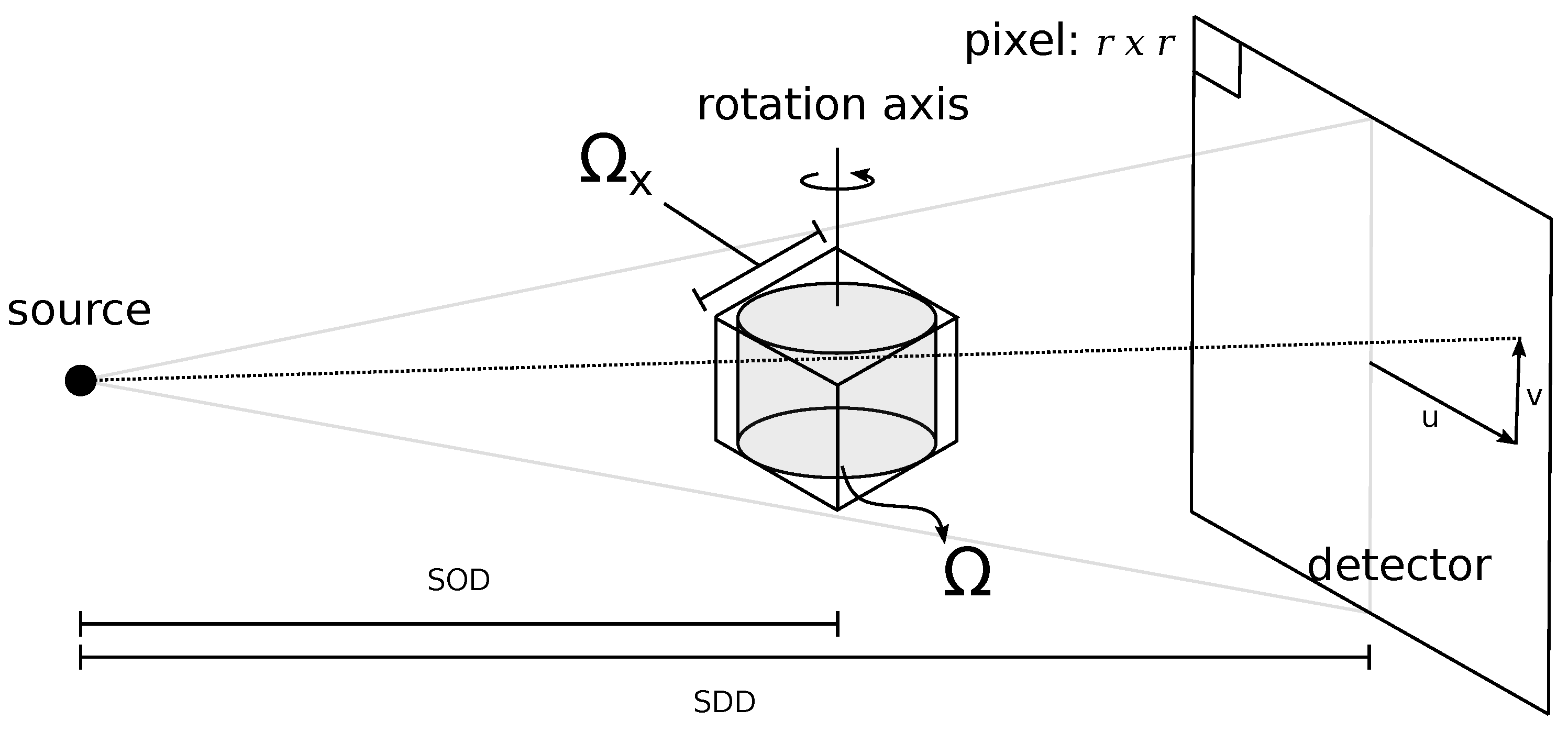
In circular cone-beam CT, an X-ray point source and flat-panel detector are fixed opposite to each other at some distance, which we refer to as the source-detector distance ($SDD$). In between, at a distance $SOD$ (source-object distance) to the source, the object under study is mounted on a rotation stage. Equivalently, the object can be fixed while the source and detector rotate around it. In either case, X-ray images are acquired at discrete angles during rotation. The resulting stack of pictures is called the projection dataset. The setup is displayed in Figure 1.

Cone beam tomography can be modeled as follows. Let the object function $f:\Omega \to \mathbb{R}$ represent the density of an unknown 3D volume supported on $\Omega \subset {\mathbb{R}}^3$. From the frame of reference of the object, the formation of the projection on the detector is given by

$$\begin{array}{c}\hfill P_{\theta }(u,v)={\int }_0^{1}f(l(t))\mathrm{d}t,\end{array}$$

(1)

where $l(t):[0,1]\to {\mathbb{R}}^3$ is the parameterization of the line segment connecting the position of the source at angle $\theta$ with position $(u,v)$ on the detector.

In practice, only a finite number $N_{\theta }$ of projections are acquired on a discrete grid of $N_u\times N_v$ detector pixels of size $r\times r$. Hence, the projection data can be described by a vector $\mathbf{p}\in {\mathbb{R}}^m,m=N_{\theta }\times N_u\times N_v$. Likewise, the object f is represented by a three-dimensional voxel grid $\mathbf{x}\in {\mathbb{R}}^{N_{\mathbf{x}}\times N_{\mathbf{x}}\times N_{\mathbf{x}}}$ describing a physical volume ${\Omega }_{\mathbf{x}}\supseteq \Omega$. In this paper, solely for ease of exposition, we choose all grids to be cubes. The physical dimensions of a single voxel, the voxel size, is naturally determined by the number of voxels in $\mathbf{x}$ and choice of ${\Omega }_{\mathbf{x}}$, and can in principle be made arbitrarily small. The discrete formulation gives rise to the linear inverse problem

$$\begin{array}{c}\hfill \mathbf{A}\mathbf{x}=\mathbf{p},\end{array}$$

(2)

with $\mathbf{A}=(a_{ij})$ an $m\times n$ matrix where $a_{ij}$ represents the contribution of volume voxel j to detector pixel i. The goal of tomographic reconstruction is to estimate $\mathbf{x}$ such that it matches the $N_{\mathbf{x}}\times N_{\mathbf{x}}\times N_{\mathbf{x}}$ voxel discretization of f.

For the circular cone beam trajectory, several methods exist to compute $\mathbf{x}$ from projections $\mathbf{p}$. One of these methods is the widely used Feldkamp–Davis–Kress (FDK) algorithm [20], $\mathbf{FDK}:{\mathbb{R}}^{N_{\theta }\times N_u\times N_v}\to {\mathbb{R}}^{N_{\mathbf{x}}\times N_{\mathbf{x}}\times N_{\mathbf{x}}}$, which computes

$$\begin{array}{c}\hfill \tilde{\mathbf{x}}=\mathbf{FDK}\left(\mathbf{p}\right)={\mathbf{A}}^T{(\mathbf{h}\ast \tilde{\mathbf{p}})}_{1D},\end{array}$$

(3)

where ${\mathbf{A}}^T\in {\mathbb{R}}^{n\times m}$, the transpose of $\mathbf{A}$, is the discrete backprojection of $\mathbf{p}$ onto $\mathbf{x}$, $\mathbf{h}\in {\mathbb{R}}^{N_u}$ is the convolution kernel associated with the FDK algorithm, and ${(\mathbf{h}\ast \tilde{\mathbf{p}})}_{1D}$ is the horizontal one-dimensional convolution of $\mathbf{h}$ with $\tilde{\mathbf{p}}$, a weighted version of $\mathbf{p}$ with diminished intensity at higher distance from the detector center. The FDK algorithm is computationally efficient and results in accurate reconstructions when the projection data have a low noise profile and have been acquired from a sufficient number of angles.

The resolution of the reconstruction cannot be arbitrarily improved by choosing a finer reconstruction grid. Even in the absence of noise and other effects, the minimal voxel size is limited by the detector pixel size [21]

$$\begin{array}{c}\hfill v=r·\frac{\mathrm{SOD}}{\mathrm{SDD}}.\end{array}$$

(4)

The angular resolution of the CT scan also influences the voxel size. The number of angles from which the projection data has been acquired also influences the minimal voxel size, but, when a sufficiently large number of angles has been used, the voxel size as determined in Equation (4) is not further limited [22].

In addition to the detector pixel size, multiple optical phenomena influence the formation of projection images. Many of these optical effects introduce a blurring effect on the projection images. For instance, pixel cross-talk causes an element of the photo-multiplier array to measure some fraction of the incoming photons of its neighboring pixels [23]. Cross-talk can occur both in the scintillator, where the high-energy photons are converted into the visible spectrum, and in the photo-sensor itself. Blurring can also be introduced when the focal spot, the region where the X-rays originate from, is a larger disc-like region rather than a point source [7], Chapter 9. These optical effects can be modeled by a point spread function (PSF), e.g., a 2D Gaussian filter, describing the projection on the detector of a point-like object. A consequence of these optical effects is that the effective resolution on the detector is lower than the pixel resolution, thereby increasing the effective voxel size [7].

Even though detector resolution is limited, Equation (4) shows that the voxel resolution can be increased by modifying the acquisition geometry. The projection of a feature located on the rotation axis has a magnification factor of

$$\begin{array}{c}\hfill \alpha =\frac{\mathrm{SDD}}{\mathrm{SOD}}.\end{array}$$

(5)

By moving the object closer to the source, this magnification factor is increased, which, thereby, as a consequence of Equation (4), decreases the minimal voxel size. As the object is moved closer to the source, the projections of the object may become truncated. Consequently, only a part of the object, the region of interest (ROI), is consistently projected onto the detector at every angle. This causes truncation artifacts in the reconstruction. Various techniques exist to minimize these artifacts [24,25,26,27]. Nonetheless, these methods only improve resolution in the region of interest, hence new methods are required to reconstruct the entire volume at high resolution.

2.2. Deep Convolutional Neural Networks

A recently proposed strategy to improve the resolution of photographic images is the use of deep convolutional neural networks (CNNs) [17]. This class of machine learning algorithms processes the image by applying multiple convolution kernels and saves the intermediate results in layers. Each layer consists of several images, and is computed by convolving the previous layer with learned kernels, adding a scalar bias term, and applying a nonlinear activation function to each pixel. The network

$$\begin{array}{c}\hfill {Net}_{C,\phi }:{\mathbb{R}}^{C\times N\times N}\to {\mathbb{R}}^{N\times N}\end{array}$$

(6)

is trained to find a set of parameters $\widehat{\phi }\in \Phi$ such that it best transforms a stack of C images into a desired image of $N\times N$ pixels. In modern CNN architectures, the number of parameters can range up to millions.

The training procedure applies the network to a training set of input data, ${(x_i)}_{i=1}^n$, and compares the output to target data ${(z_i)}_{i=1}^n$, where the goal is to minimize a user-specified empirical loss function L. In this paper, we use the pixel-wise mean square error

$$\begin{array}{c}\hfill L(\phi )=\frac{1}{n}\sum _{i=1}^n||{{Net}_{C,\phi }(x_i)-z_i||}_2^2.\end{array}$$

(7)

Training is not usually carried out to completion, i.e., the training is stopped before the absolute minimum of L is attained on the training set. This is done to prevent overfitting the network to the training data. When the network is overfit, the empirical loss is low for data in the training set, but high for data not included in the training set. The performance of a network that is being trained is commonly tested on a validation set that is not part of the training set. Once the performance on the validation set stops improving, training is stopped. An alternative to using a validation set is early stopping, where training is stopped at some predetermined time.

Most existing state-of-the-art CNNs process 2D images. To process 3D volumes, we can subdivide the input and target voxel grids ${\tilde{\mathbf{x}}}^{\mathrm{input}}$ and ${\tilde{\mathbf{x}}}^{\mathrm{target}}$ into 2D horizontal slices. As input, the network is provided with a slab containing not just a single input slice but also surrounding slices, supplying the network with quasi-3D information. Although network architectures exist that process entire 3D volumes at once, their memory requirements are challenging when applied to voxel grids with sizes that are common in tomography.

3. Method

In this section, we describe the main contribution of this paper: an integrated data acquisition and machine learning approach for improving resolution in cone-beam tomography. Our approach consists of several steps. First, we perform a standard CT scan of the object under study. In addition to a standard CT scan, we acquire additional projection images with the object moved closer to the radiation source. Second, we reconstruct the entire volume at low resolution. Next, using both projection datasets, we reconstruct a region of interest at high resolution. These two reconstructions are used to train a neural network to compute a mapping between the low-resolution volume in the region of interest and its high-resolution counterpart. The trained neural network is then applied to the entire low-resolution volume to obtain a final high-resolution volume representation. This process is illustrated in Figure 2. In the next subsections, we describe the steps of our data acquisition and reconstruction strategy in detail.

3.1. Data Acquisition

Our data acquisition protocol consists of two scans. The first scan with magnification factor ${\alpha }_{\mathrm{low}}=\raisebox{1ex}{$SDD$}\!\left/ \!\raisebox{-1ex}{$SOD$}\right.$ is a standard circular cone beam scan and yields projection dataset ${\mathbf{p}}^{\mathrm{low}}$, as shown in Figure 1. In addition to the standard acquisition, we propose to acquire an additional projection dataset ${\mathbf{p}}^{\mathrm{high}}$. Here, the object is moved closer to the source such that the resulting projection on the detector has a magnification factor of ${\alpha }_{\mathrm{high}}=\raisebox{1ex}{$SDD$}\!\left/ \!\raisebox{-1ex}{$SO{D}_2$}\right.$. Now, only a region of interest ${\Omega }_{\mathrm{ROI}}\subseteq \Omega \subseteq {\mathbb{R}}^3$ is in full view on the detector at all times, as is depicted in Figure 3. The addition of the second projection dataset ${\mathbf{p}}^{\mathrm{high}}$ permits the high-resolution reconstruction of a rectangular sub-region of the region of interest. This is described below.

3.2. Reconstruction

From the acquired datasets, two reconstructions are computed. The first reconstruction contains the entire object at low resolution, and the second reconstruction describes the region of interest at high resolution. Because these reconstructions are later used for the training of a neural network, we ensure that their voxel grids are aligned.

The dimensions of the low-resolution reconstruction grid are determined using the pixel size r and the physical dimensions $\Omega$ of the object. We calculate the effective voxel size $v_{\mathrm{low}}=\raisebox{1ex}{$r$}\!\left/ \!\raisebox{-1ex}{${\alpha }_{\mathrm{low}}$}\right.$ using Equations (4) and (5). Given the voxel size, the shape of the voxel grid ${\mathbf{x}}^{\mathrm{low}}$, $N_{\mathrm{low}}\times N_{\mathrm{low}}\times N_{\mathrm{low}}$, is established such that its real-world volume ${\Omega }_{\mathrm{low}}\subset {\mathbb{R}}^3$ covers the object, i.e., $\Omega \subseteq {\Omega }_{\mathrm{low}}$. On this grid, the low-resolution reconstruction is computed using the FDK algorithm

$$\begin{array}{cc}\hfill {\tilde{\mathbf{x}}}^{\mathrm{low}}& =\mathbf{FDK}\left({\mathbf{p}}^{\mathrm{low}}\right)\in {\mathbb{R}}^{N_{\mathrm{low}}^3}.\hfill \end{array}$$

(8)

Next, we determine the shape and voxel size $v_{\mathrm{high}}$ of the high-resolution voxel grid ${\mathbf{x}}^{\mathrm{high}}$. We set the voxel size to equal $v_{\mathrm{high}}=v_{\mathrm{low}}/k$, where k equals ${\alpha }_{\mathrm{high}}/{\alpha }_{\mathrm{low}}$ rounded to the nearest integer. In practice, magnification factors ${\alpha }_{\mathrm{low}}$ and ${\alpha }_{\mathrm{high}}$ can be carefully chosen to avoid the need for rounding. The voxel size $v_{\mathrm{high}}$ is close to the limit defined by Equation (4), since, by Equation (5), we have

$$\begin{array}{c}\hfill v_{\mathrm{high}}=\frac{v_{\mathrm{low}}}{k}\approx v_{\mathrm{low}}\frac{{\alpha }_{\mathrm{low}}}{{\alpha }_{\mathrm{high}}}=\frac{r}{{\alpha }_{\mathrm{low}}}\frac{{\alpha }_{\mathrm{low}}}{{\alpha }_{\mathrm{high}}}=\frac{r}{{\alpha }_{\mathrm{high}}}.\end{array}$$

(9)

We fix the physical volume of the high-resolution grid, ${\Omega }_{\mathrm{high}}$, to be contained in the region of interest, i.e., ${\Omega }_{\mathrm{high}}\subseteq {\Omega }_{\mathrm{ROI}}$, and set its shape, $N_{\mathrm{high}}\times N_{\mathrm{high}}\times N_{\mathrm{high}}$, such that $N_{\mathrm{high}}$ is divisible by k. Now, voxels from ${\mathbf{x}}^{\mathrm{low}}$ relate to cubes of $k\times k\times k$ voxels in ${\mathbf{x}}^{\mathrm{high}}$. This assists in modeling the forward projection of the second scan.

As shown in Figure 3, the rays forming the projection data, ${\mathbf{p}}^{\mathrm{high}}$, have been transmitted through both ${\Omega }_{\mathrm{high}}$ and $\Omega \backslash {\Omega }_{\mathrm{high}}$. This is modeled by the discrete linear equation

$$\begin{array}{cc}\hfill {\mathbf{p}}^{\mathrm{high}}& \approx {\mathbf{A}}^{(\mathrm{high})}{\mathbf{x}}^{\mathrm{high}}+{\mathbf{A}}^{(\mathrm{low}\to \mathrm{high})}\mathbf{M}{\mathbf{x}}^{\mathrm{low}},\hfill \end{array}$$

(10)

where $\mathbf{M}\in {\mathbb{R}}^{N_{\mathrm{low}}^3\times N_{\mathrm{low}}^3}$ is a matrix that masks all voxels in ${\mathbf{x}}^{\mathrm{low}}$ that are contained in ${\Omega }_{\mathrm{high}}$. In other words, $\mathbf{M}$ is a diagonal matrix where the diagonal is 0 on row i if voxel i of the large grid ${\mathbf{x}}^{\mathrm{low}}$ overlaps ${\Omega }_{\mathrm{high}}$, and is 1 elsewhere. The matrix ${\mathbf{A}}^{(\mathrm{low}\to \mathrm{high})}=(a_{ij})$ is defined such that $a_{ij}$ represents the contribution of the low-resolution volume voxel ${\mathbf{x}}_j^{\mathrm{low}}$ to detector pixel ${\mathbf{p}}_i^{\mathrm{high}}$ at magnification ${\alpha }_{\mathrm{high}}$. The matrix ${\mathbf{A}}^{(\mathrm{high})}$ similarly defines the projection of the high-resolution volume ${\mathbf{x}}^{\mathrm{high}}$ at magnification ${\alpha }_{\mathrm{high}}$.

To reconstruct ${\mathbf{x}}^{\mathrm{high}}$, we subtract the reprojection of the masked reconstruction $\mathbf{M}{\tilde{\mathbf{x}}}^{\mathrm{low}}$ from the acquired high-resolution projection data

$$\begin{array}{cc}\hfill \widehat{\mathbf{p}}& ={\mathbf{p}}^{\mathrm{high}}-{\mathbf{A}}^{(\mathrm{low}\to \mathrm{high})}\mathbf{M}{\tilde{\mathbf{x}}}^{\mathrm{low}}.\hfill \end{array}$$

(11)

Next, we apply the FDK algorithm to the processed projection data to obtain the reconstruction

$$\begin{array}{cc}\hfill {\tilde{\mathbf{x}}}^{\mathrm{high}}& =\mathbf{FDK}\left(\widehat{\mathbf{p}}\right)\in {\mathbb{R}}^{N_{\mathrm{high}}^3}.\hfill \end{array}$$

(12)

In a conventional FDK reconstruction, the outside contributions of $\Omega \backslash {\Omega }_{\mathrm{high}}$ to the projection data ${\mathbf{p}}^{\mathrm{high}}$ cause truncation artifacts. Because we have approximately removed these contributions, we can apply the FDK algorithm to obtain a high-resolution reconstruction of the region of interest. Note that similar subtraction methods have been proposed before to remove truncation artifacts in region-of-interest tomography [25,27,28]. Some artifacts may occur on the border of the region of interest, which may be due to the specifics of the interpolation kernel that is used in the forward projection ${\mathbf{A}}^{(\mathrm{low}\to \mathrm{high})}$ or due to discontinuity at the image borders enhanced by the FDK filter kernel. Water cylinder extrapolation or truncation robust FBP methods like [29] may alleviate these artifacts. These artifacts are not a problem in practice, as the affected border voxels may be ignored.

3.3. Machine Learning

At this point in the process, the tomographic reconstruction method yields a low-resolution voxel grid ${\tilde{\mathbf{x}}}^{\mathrm{low}}$ and a high-resolution voxel grid ${\tilde{\mathbf{x}}}^{\mathrm{high}}$. For the neural network to match the low-resolution input to the high-resolution target, it is necessary that both input and target relate to the same physical space, and have the same voxel size. In this section, we outline how ${\tilde{\mathbf{x}}}^{\mathrm{low}}$ and ${\tilde{\mathbf{x}}}^{\mathrm{high}}$ are processed to match in physical space and voxel size. We also describe the training procedure, and motivate the choice of neural network architecture.

The voxel grid ${\tilde{\mathbf{x}}}^{\mathrm{low}}$ corresponds to the physical space ${\Omega }_{\mathrm{low}}$ and ${\tilde{\mathbf{x}}}^{\mathrm{high}}$ corresponds to ${\Omega }_{\mathrm{high}}$. To serve as input data for neural network training, we use the voxels from ${\tilde{\mathbf{x}}}^{\mathrm{low}}$ that are contained in ${\Omega }_{\mathrm{high}}$. We denote this restriction operation by $\mathbf{R}:{\mathbb{R}}^{N_{\mathrm{low}}^3}\to {\mathbb{R}}^{N_{\mathrm{high}}^3/k^3}$. The resulting voxel grid

$$\begin{array}{c}\hfill {\tilde{\mathbf{x}}}_{\mathrm{ROI}}^{\mathrm{low}}=\mathbf{R}({\tilde{\mathbf{x}}}^{\mathrm{low}})\in {\mathbb{R}}^{N_{\mathrm{high}}^3/k^3}\end{array}$$

(13)

corresponds to the physical volume ${\Omega }_{\mathrm{high}}$, and each of its voxels can thus be matched with voxels from ${\tilde{\mathbf{x}}}^{\mathrm{high}}$.

The voxel sizes of ${\tilde{\mathbf{x}}}_{\mathrm{ROI}}^{\mathrm{low}}$ and ${\tilde{\mathbf{x}}}^{\mathrm{high}}$ can be equalized by either up-sampling the input data ${\tilde{\mathbf{x}}}_{\mathrm{ROI}}^{\mathrm{low}}$ or down-sampling the target data ${\tilde{\mathbf{x}}}^{\mathrm{high}}$. We present both options, which we designate as method A and method B, respectively. By up-sampling the input data by a factor k with an interpolation method ${\mathbf{U}}_k:{\mathbb{R}}^{N_{\mathrm{high}}^3/k^3}\to {\mathbb{R}}^{N^3}$ with $N=N_{\mathrm{high}}$, we obtain training data on a fine grid

$$\begin{array}{ccc}\hfill {\tilde{\mathbf{x}}}^{\mathrm{input}}& ={\mathbf{U}}_k({\tilde{\mathbf{x}}}_{\mathrm{ROI}}^{\mathrm{low}})\in {\mathbb{R}}^{N^3},\hfill & \hfill (\mathrm{method}\mathrm{A})\end{array}$$

(14)

$$\begin{array}{cc}\hfill {\tilde{\mathbf{x}}}^{\mathrm{target}}& ={\tilde{\mathbf{x}}}^{\mathrm{high}}\in {\mathbb{R}}^{N^3}.\hfill \end{array}$$

(15)

By down-sampling the target data by a factor k with an interpolation method ${\mathbf{D}}_k:{\mathbb{R}}^{N_{\mathrm{high}}^3}\to {\mathbb{R}}^{N^3}$ with $N=N_{\mathrm{high}}/k$, we obtain training data on a coarse grid

$$\begin{array}{ccc}\hfill {\tilde{\mathbf{x}}}^{\mathrm{input}}& ={\tilde{\mathbf{x}}}_{\mathrm{ROI}}^{\mathrm{low}}\in {\mathbb{R}}^{N^3},\hfill & \hfill (\mathrm{method}\mathrm{B})\end{array}$$

(16)

$$\begin{array}{cc}\hfill {\tilde{\mathbf{x}}}^{\mathrm{target}}& ={\mathbf{D}}_k({\tilde{\mathbf{x}}}^{\mathrm{high}})\in {\mathbb{R}}^{N^3}.\hfill \end{array}$$

(17)

The interpolation methods ${\mathbf{U}}_k$ and ${\mathbf{D}}_k$ are open to choice. Various methods can be used, including, for instance, cubic interpolation. The up- and down-sampling operations are illustrated in Figure 4.

The properties of the acquired projection data can be used to inform the choice whether to up-sample the input (method A), or down-sample the target (method B). When optical blurring on the detector is negligible, the small-scale features that can be seen in ${\tilde{\mathbf{x}}}^{\mathrm{high}}$ will be hard to visualize on the coarse grid of ${\tilde{\mathbf{x}}}_{\mathrm{ROI}}^{\mathrm{low}}$. Therefore, it is recommended to use method A where ${\tilde{\mathbf{x}}}^{\mathrm{target}}$ is defined on a fine grid. If, on the other hand, optical blurring limits the effective resolution of ${\tilde{\mathbf{x}}}_{\mathrm{ROI}}^{\mathrm{low}}$, and its resolution can be improved without reducing the voxel size, then it is recommended to use method B, where the grid size is smaller, and training and applying the network is thus computationally faster. The differences between the input and target grids are summarized in the first three columns of

Table 1. An overview of the grid sizes of method A, where the input is up-sampled, and method B, where the target is down-sampled. The grid size and input are tabulated for the training phase and the processing phase, in which the final output is calculated. The grid size is in number of voxels. The processing grid size is the size of the output ${\tilde{\mathbf{x}}}^{\mathrm{final}}$ when the network is applied to ${\tilde{\mathbf{x}}}^{\mathrm{low}}$, and s is the number of additional input slices that the network takes as input.

	Training			Processing
	Grid Size (${\mathit{N}}^3$)	Input (${\tilde{\mathbf{x}}}^{\mathbf{input}}$)	Target (${\tilde{\mathbf{x}}}^{\mathbf{target}}$)	Grid Size (${\mathit{N}}_{\mathbf{final}}^3$)	Input
Method A	$N_{\mathrm{high}}^3$	${\mathbf{U}}_k({\tilde{\mathbf{x}}}_{\mathrm{ROI}}^{\mathrm{low}})$	${\tilde{\mathbf{x}}}^{\mathrm{high}}$	${(k{N}_{\mathrm{low}}-2s)}^3$	${\mathbf{U}}_k({\tilde{\mathbf{x}}}^{\mathrm{low}})$
Method B	$N_{\mathrm{high}}^3/k^3$	${\tilde{\mathbf{x}}}_{\mathrm{ROI}}^{\mathrm{low}}$	${\mathbf{D}}_k({\tilde{\mathbf{x}}}^{\mathrm{high}})$	${(N_{\mathrm{low}}-2s)}^3$	${\tilde{\mathbf{x}}}^{\mathrm{low}}$

.

The input and target voxel grids ${\tilde{\mathbf{x}}}^{\mathrm{input}}$ and ${\tilde{\mathbf{x}}}^{\mathrm{target}}$ serve to train the convolutional neural network. The voxel grids ${\tilde{\mathbf{x}}}^{\mathrm{input}}$ and ${\tilde{\mathbf{x}}}^{\mathrm{target}}$ are divided into slices ${\tilde{\mathbf{x}}}_i^{\mathrm{input}},{\tilde{\mathbf{x}}}_i^{\mathrm{target}},i=1,\dots ,N$ as illustrated in Figure 4. In this article, ${\mathbf{x}}_i$ denotes both a single voxel at position i and a horizontal slice i of a voxel grid $\mathbf{x}$. The surrounding text always distinguishes between a voxel and a slice.

The input slices are combined into slabs $[{{\tilde{\mathbf{x}}}_j^{\mathrm{input}}]}_{j=i-s}^{i+s},i=s+1,\dots ,N-s,$ containing the input slice and the s slices above and below. The target slices are not combined into slabs. The training procedure now minimizes

$$\begin{array}{c}\hfill L_s(\phi )=\frac{1}{N}\sum _{i=s+1}^{N-s}\left|\right|{{Net}_{2s+1,\phi }\left([{{\tilde{\mathbf{x}}}_j^{\mathrm{input}}]}_{j=i-s}^{i+s}\right)-{\tilde{\mathbf{x}}}_i^{\mathrm{target}}\left|\right|}_2^2,\end{array}$$

(18)

which yields the set of parameters, $\widehat{\phi }$. Other norms, such as the L1 norm, could also be used.

Multiple deep network architectures can be used to improve the quality of reconstructions [30,31,32,33]. One of these is the mixed-scale dense (MS-D) network, which is a neural network architecture specifically developed for scientific settings. The mixed-scale dense network has several properties that make it well-suited for our method. The MS-D network has relatively few parameters compared to other neural network structures, making it easier to train and less likely to overfit. This is especially useful if a small training set is available, and no part of the training set is sacrificed to serve as a validation set, as is the case in this paper. Another advantage is that the MS-D network maximally reuses the intermediate images in each layer, thus requiring fewer intermediate images compared to other deep convolutional neural network architectures. Therefore, the MS-D network can transform large images using less memory and computation time compared to other popular convolutional neural network architectures [33]. Finally, the network has shown good results for removing noise and other artifacts from tomographic images when a large training set of similar objects scanned at high dose is available. This is described in [34], where the network was applied to tomographic images reconstructed from a dataset of parallel beam projections, rather than cone beam projections.

3.4. Improving Resolution

After training the network, a set of network parameters $\widehat{\phi }$ is obtained. The trained neural network ${Net}_{\widehat{\phi }}$ is applied to the initially reconstructed low-resolution volume ${\tilde{\mathbf{x}}}^{\mathrm{low}}$ to obtain a final volume representation ${\tilde{\mathbf{x}}}^{\mathrm{final}}$. This process consists of several steps. If the training input has been up-sampled using method A, then the reconstruction ${\tilde{\mathbf{x}}}^{\mathrm{low}}$ must likewise be up-sampled to ${\mathbf{U}}_k({\tilde{\mathbf{x}}}^{\mathrm{low}})$, which is k times larger in every dimension. If method B has been used, no up-sampling of the reconstruction is necessary. The resulting voxel grid is processed by the network slice by slice. These slices must be collected in slabs containing s slices above and below the input slice. This influences the output size, since the top and bottom s slices of ${\tilde{\mathbf{x}}}^{\mathrm{low}}$ do not have enough surrounding slices to be processed by the network. This is usually not a problem because s is small ($s<10$) and the low-resolution grid can be chosen large enough that any important features are at some distance from the top and bottom. Finally, the network can be applied to each of these slabs in turn, the result of which we collect into ${\tilde{\mathbf{x}}}^{\mathrm{final}}$. In summary, this process results in the final volume representation

$$\begin{array}{ccc}\hfill {\tilde{\mathbf{x}}}^{\mathrm{final}}& =[{{Net}_{2s+1,\widehat{\phi }}\left([{U_K{\left({\tilde{\mathbf{x}}}^{\mathrm{low}}\right)}_j]}_{j=i}^{i+2s}\right)]}_{i=1}^{N_{\mathrm{final}}}\hfill & \hfill (\mathrm{Method}\mathrm{A}),\\ \hfill {\tilde{\mathbf{x}}}^{\mathrm{final}}& =[{{Net}_{2s+1,\widehat{\phi }}\left([{{\tilde{\mathbf{x}}}_j^{\mathrm{low}}]}_{j=i}^{i+2s}\right)]}_{i=1}^{N_{\mathrm{final}}}\hfill & \hfill (\mathrm{Method}\mathrm{B}).\end{array}$$

For both methods, the size of the final grid ${\tilde{\mathbf{x}}}^{\mathrm{final}}$ is summarized in Table 1.

4. Results

We evaluate the accuracy of our method on simulated and experimental data, which is described below. Before going through the specifics of each experiment, we first provide details on the steps that all experiments have in common.

Data acquisition For each experiment, three projection datasets are acquired. The first projection dataset has the entire object in the field of view and has a low magnification factor ${\alpha }_{\mathrm{low}}$. The second and third projection datasets are acquired of a central and upper region of interest and have a higher magnification factor ${\alpha }_{\mathrm{high}}$. This is illustrated in Figure 5.

Reconstruction In all experiments, high-resolution reconstructions are computed of a central and upper region of interest to serve as target data for the training set and test set, respectively. A low-resolution reconstruction is computed of the entire object, which serves as input data for both training and testing. In all experiments, the low-resolution voxels are $k=4$ times as large as the high-resolution voxels. FDK reconstructions were computed using the ASTRA toolbox [35].

Up- and down-sampling The up- and down-sampling of the reconstructed volumes can be performed in various ways. In the experiments, up-sampling in method A is carried out by nearest-neighbor up-sampling, where each voxel is repeated k times in each direction. Empirically, we found this to be sufficient, as cubic up-sampling did not improve the quality of the network output. Down-sampling of the target voxel grid in method B is carried out using three-dimensional cubic interpolation, where the image is interpolated to a coarser grid using polynomials of degree at most 3 determined by a window of $4\times 4\times 4$ voxels.

Neural network implementation For each experiment, three separate networks are trained using: (i) method A and a single input slice, (ii) method A and a slab of nine input slices, (iii) method B and a single input slice. The MS-D network is implemented in PyTorch [36]. Each trained network has 100 single-channel intermediate layers, and the convolution in layer i is dilated by $d_i=1+(imod10)$, as is described in [33]. The network has 45,652 parameters when there is a single input slice, and it has 52,948 parameters when the input is a slab of nine slices.

Training procedure The network is trained on the central region of interest. Because we chose not to use a validation set, a criterion was set for early stopping. In all experiments, training finished after two days or 1000 epochs, whichever came first. All networks are trained from scratch in each experiment. The training procedure minimizes the mean square error between the output and target images, and the networks are trained using the ADAM algorithm [37] with a mini-batch size of one. The network output is evaluated on a test set containing the low- and high-resolution reconstructions of the upper region of interest. The training and test set are thus non-overlapping.

Metrics and evaluation On both datasets, the on-the-fly machine learning approach is evaluated using the structural similarity index (SSIM) [38] and the mean square error (MSE) metrics. These metrics are used to compare the output slices of the networks to target slices from the upper ROI reconstruction. To compare methods A and B on the same grid, the output volume of method B is cubically up-sampled before computing the MSE and SSIM metrics. The output slices of method A are not processed, since they are the same size as the target slices of the test set. Both metrics are computed slice by slice and averaged. To prevent the influence of reconstruction artifacts at the boundaries of the high-resolution reconstructions, all metrics are calculated on pixels that are at least eight pixels from the boundary of the volume. Likewise, all displayed images are cropped to remove eight pixels from all sides. The error metrics of our approach are compared to a baseline: a full-volume three-dimensional cubic up-sampling of the low-resolution input volume. We visually compare all methods on the central slice of the upper ROI reconstruction on both the simulated and the experimental data.

All computations were performed on a server with 192 GB of RAM and four Nvidia GeForce GTX 1080 Ti GPUs (Nvidia, Santa Clara, CA, USA) or on a workstation with 64 GB of RAM and one Nvidia GeForce GTX 1070.

4.1. Simulations

First, we investigated the performance of the proposed on-the-fly machine learning technique on simulated tomographic data.

Simulation phantom A foam ball simulation phantom was generated by removing 90,000 randomly-placed non-overlapping spheres from a large sphere made of one material. The foam ball has diameter 1. All other dimensions in the simulation are relative to this unit length. The radius of the random spheres ranges between $0.0025$ and $0.2$. The central slice of this phantom is displayed in Figure 6.

Data simulation Using the foam phantom, three projection datasets were computed. For the first projection dataset, which has the entire foam ball in the field of view, the source-object distance is equal to the source-detector distance, yielding a magnification factor of ${\alpha }_{\mathrm{low}}=1$. In practice, having an equal source-object and source-detector distance is not possible, since the detector and object would share the same physical space. In simulations, however, this is both possible and natural, since it results in a minimal voxel size that is equal to the detector pixel size. The second and third projection dataset were acquired at a magnification factor of ${\alpha }_{\mathrm{high}}=4$.

To simulate how our method copes with optical phenomena, another set of projections was created by post-processing the projections using a Gaussian blur with standard deviation of two pixels. The Gaussian blur convolves the projection images with a 2D filter defined by $g(x)=exp(-{||x||}^2/2{\sigma }^2)/\sqrt{2\pi {\sigma }^2}$, where $\sigma$ is the chosen standard deviation. We refer to the blurred data as optics-limited, and to the non-blurred data as pixel-limited.

The projections were carried out using the GPU-accelerated cone_balls software package, which we have made available as an open source package [39]. This package analytically computes the linear cone beam projection of solid spheres of constant density. For each dataset, 1500 projections were acquired over 360 degrees on a virtual detector with $1000\times 1000$ pixels. For each detector pixel, four rays were cast through the phantom, and their projection values were averaged.

Processing The reconstruction and training of the foam phantom was performed as described before in Section 4. The details are summarized in

Table 2. A summary of the pixel and voxel grids used for the reconstructions of the full object and regions of interest (ROIs). For each dataset, the network was trained by up-sampling the input (method A) with a slab of nine slices and one slice as input, and by down-sampling the target (method B) with a slab of one slice as input.

	Foam	Foam	Oatmeal
	Pixel-Limited	Optics-Limited
Detector
Shape	$1000\times 1000$	$1000\times 1000$	$1536\times 1944$
Pixel size	$0.0012$	$0.0012$	$75\mathsf{\mu }\mathrm{m}$
Number of angles	1500	1500	2000
Full object
Grid shape	$1064\times 1064\times 1064$	$1064\times 1064\times 1064$	$1647\times 2084\times 2084$
Voxel size	$0.0012$	$0.0012$	$68.26\mathsf{\mu }\mathrm{m}$
Central ROI
Grid shape	$888\times 664\times 664$	$888\times 664\times 664$	$1364\times 1304\times 1304$
Voxel size	$0.0003$	$0.0003$	$17.07\mathsf{\mu }\mathrm{m}$
Top ROI
Grid shape	$880\times 664\times 664$	$880\times 664\times 664$	$1364\times 1304\times 1304$
Voxel size	$0.0003$	$0.0003$	$17.07\mathsf{\mu }\mathrm{m}$
Training epochs
Method A 9 slices	230	230	30
Method A 1 slice	260	250	40
Method B 1 slice	1000	1000	950

. Methods A and B are evaluated on the upper ROI reconstruction, and compared below for both the pixel-limited and optics-limited case.

Evaluation For the simulated data, the MSE and SSIM metrics are computed between the network outputs and the original phantom data, rather than the high-resolution reconstruction. As the SSIM metric is designed to operate on images with a fixed intensity interval, we clip the network outputs such that all images have the same minimum and maximum intensity as the phantom data. Similarly, the images displayed in Figure 7 are clipped to the range $[0,1]$. The MSE metrics are calculated on the unclipped data.

The quantitative results for the foam phantom are given in

Table 3. Foam ball phantom: comparison of the MSE and SSIM between the output of the three approaches described in this section and cubic up-sampling. For each dataset and metric, the best results are shown in bold.

Dataset	Method A		Method A		Method B		Cubic up-Sampling
	Slab: 9 Slices		Slab: 1 Slice		Slab: 1 Slice
	MSE	SSIM	MSE	SSIM	MSE	SSIM	MSE	SSIM
Pixel-limited	0.0044	0.9578	0.0089	0.9281	0.0111	0.8065	0.0125	0.6893
Optics-limited	0.0143	0.8275	0.0154	0.8220	0.0178	0.8135	0.0463	0.6038

. Both variants of method A significantly outperform cubic up-sampling on both MSE and SSIM metrics. On the pixel-limited dataset, the SSIM score of method B is lower than the methods A but higher than cubic up-sampling. The fine scale features in the pixel-limited high-resolution image can simply not be represented on the coarser grid that method B operates on. On the optics-limited dataset, on the other hand, the SSIM score of method B is comparable to the SSIM scores of methods A, and is significantly higher than that of cubic up-sampling.

In Figure 7, the methods are visually compared on both the pixel-limited dataset and the optics-limited dataset. In the pixel-limited dataset, the low-resolution input suffers from partial volume effects, where some voxels contain more than one material. In this case, the foam and void contributions to a voxel are averaged, which leads to jagged edges. The high-resolution data are significantly sharper, but still has some non-smooth texture in the foam and voids. The output of method A with nine input slices makes the edges as sharp as in the high-resolution image, and removes the non-smooth texture in the foam and voids. Moreover, it does not introduce any voids where there are none in the target data. Method A with one input slice performs similarly, but has some difficulty with features that are rapidly introduced in the vertical direction. This is apparent in the magnified image in Figure 7, where the top or bottom of one void in the input data are not correctly removed. As discussed before, method B performs worse than method A when the high-resolution features cannot be represented on the coarse grid.

In the optics-limited dataset, both low- and high-resolution slices are less sharp than in the pixel-limited case. Due to the additional blur on the projection data, some of the smaller features in the low-resolution image cannot easily be distinguished. Nonetheless, the output of both methods A has significantly improved resolution and is visually similar to the target slice. With few exceptions, all voids in the output are round, and, without exception, all voids in the output are also present in the target. Method B produces output that looks similar to the output of methods A, although it fuses some voids that can still be distinguished in the output of methods A.

4.2. Experimental Data

To verify the practical applicability of our approach, we have investigated the performance of our method on experimentally acquired cone-beam CT data.

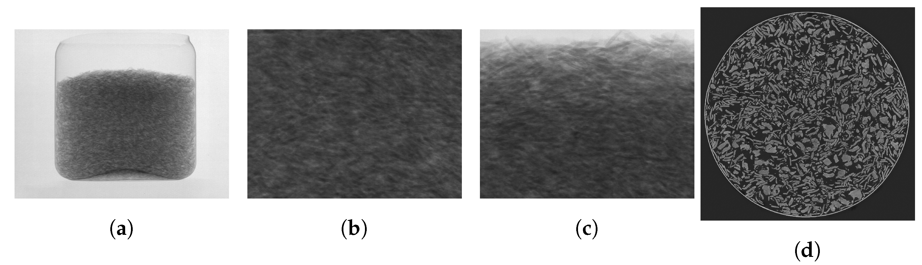
Sample A plastic jar filled with oatmeal was scanned. The oatmeal was specifically chosen for its structure, which is consistent throughout the entire object. A package of oatmeal contains thousands of flakes, which all have roughly the same dimensions and shape, but still exhibit fine-scale features, requiring high-resolution tomography to accurately capture. Projection and reconstruction images of the oatmeal are displayed in Figure 8.

Data acquisition The projection images were acquired using the custom-built and flexible CT scanner, FleX-ray Laboratory, developed by XRE NV and located at CWI [40]. The apparatus consists of a cone-beam microfocus X-ray point source that projects polychromatic X-rays onto a $1944\times 1536$ pixels, 14-bit, flat detector panel. The data was acquired over 360 degrees in circular motion with 2000 projections distributed evenly over the full circle. The projections were collected with 250 ms exposure time and the total scanning time was 11 minutes per acquisition. The tube voltage was 70 kV and the tube power was 42 W. This acquisition strategy was performed three times with magnification factors $\alpha =1.09,4.38,$ and $4.38$. Examples of the acquired projection images are displayed in Figure 8 and an overview of scanning time and emitted beam energy is given in

Table 4. The scanning times and emitted beam energy of the experiments. The third row contains an estimate of the duration of a full high-resolution scan with a detector tiling strategy, where a virtual large projection image is created by stitching the images for several detector positions. To achieve similar resolution as the high-resolution ROI scan, 16 detector positions would have to be stitched together. The emitted beam energy is used as a proxy for the radation dose absorbed by the object. The efficiency of the source $\eta$ is multiplied by the power $P=42W$ applied to the X-ray tube, and the scanning time in seconds.

	Emitted Beam Energy (J)	Scanning Time (Minutes)
Full low-resolution scan	$\eta \times$ 27,720	11
High-resolution ROI scan	$\eta \times$ 27,720	11
Full high-resolution scan	$\eta \times$ 443,520	176
(Estimate for tiling)

. The object was centered on the detector for the first two scans, and the object was moved down to capture a region of interest above the center of the object for the final scan. These data are publicly available via [41].

Processing Reconstructions were computed of the full object, a central region of interest (serving as training set), and an upper region of interest (serving as test set). An example of the central slice of the oatmeal is displayed in Figure 8d. The voxels in the full-object reconstruction are four times larger in each dimension than the voxels in the region-of-interest reconstructions. The training step was also performed in the same way as for the simulated data. The details are summarized in Table 2. Up-sampling the low-resolution region-of-interest slices to $1304\times 1304$ pixels takes roughly $0.56$ s per slice and 13 min in total using method A with one input slice. Using method B, up-sampling a single slice takes $0.03$ s, and the entire region of interest can be up-sampled in less than a minute.

Evaluation The attenuation coefficients of the voxels in the high-resolution reconstruction are contained in the range $[-0.039,0.105]$. To enable comparison of the MSE and SSIM metrics of the experimental data with the simulated data, we rescaled the attenuation coefficients of the target volume to the range $[0,1]$, and used the same scaling factors to rescale the values of all other volumes. In addition, before calculating the SSIM, all volumes are clipped to the range $[0,1]$, similar to the simulated data. Likewise, the slices displayed in Figure 9 are rescaled and clipped to the unit range.

The experimental results on the oatmeal dataset are visually compared on the central slice of the upper region of interest. This low-resolution input slice, which is displayed in Figure 9, is thus not part of the training set. The low- and high-resolution slices of the oatmeal both suffer from some noise. The high-resolution slice contains significantly more visible fine-scale features. The output of the three methods is virtually indistinguishable in the non-magnified images. In the magnified images, we see that not all fine details can be retrieved: some small features are removed and others are slightly deformed compared to the target. In the red ellipse, a large flake is visible in the low-resolution slice that appears larger than it really is due to partial volume effects. The high-resolution slice, on the other hand, shows only a small fragment of the large flake. All three networks are able to filter away a large part of the flake and retain the ridge that is visible in the high-resolution slice. The three methods significantly reduce the background noise that is present in the high-resolution target beyond what can be achieved using cubic up-sampling. Overall, all three methods sharpen features that are hard to distinguish in the input, significantly reduce the background noise, and do not introduce new features that are not present in the high-resolution slice. The quantitative results paint a similar picture, and are displayed in

Table 5. Oatmeal: comparison of the MSE and SSIM between the output of the three approaches described in this section and cubic up-sampling. The best results are shown in bold for each metric.

	Method A		Method A		Method B		Cubic up-Sampling
	Slab: 9 Slices		Slab: 1 Slice		Slab: 1 Slice
	MSE	SSIM	MSE	SSIM	MSE	SSIM	MSE	SSIM
Oatmeal	0.0027	0.4508	0.0026	0.4529	0.0025	0.4521	0.0035	0.4192

. The difference between the three proposed methods in terms of MSE and SSIM is small, whereas the cubic up-sampling performs worse on both metrics.

Comparing method A and method B, we observe a difference between simulation and experimental data. For the pixel-limited dataset, method A performs better on the MSE and SSIM metrics, and it outputs visually more appealing and accurate results. For the real-world data, however, there appears to be qualitatively little difference between method B and method A. In this case, the coarse voxel grid seems fine enough to represent almost all details that can be reconstructed.

4.3. Comparison with Other Network Structures

In this section, we compare the results of the MS-D network to the widely used U-net approach described in [30] on both the simulated and experimental data. The data acquisition and reconstruction procedures remain unchanged, and the U-net is trained on the low- and high-resolution data for two days or 1000 epochs, whichever comes first. As before, the metrics on the simulated data are computed based on the original phantom and the output of the network, and the metrics on the experimental data are computed based on the high-resolution target and the output of the network.

Neural network implementation The U-net network is implemented in PyTorch, and is based on a widely available open source implementation. We have provided our code as an open source package [42]. This implementation of the U-net architecture is almost identical to that described in [30]: the images are down-sampled four times using $2\times 2$ max-pooling, the “up-convolutions” have trainable parameters, and the convolutions have $3\times 3$ kernels. Like [43], this implementation uses batch normalization before each ReLU. Moreover, the smallest image layers are 512 channels instead of 1024 channels, and zero-padding is used instead of reflection-padding. An adaptation was made to allow the network to process images whose width or height was not divisible by 16: these images were padded to the right dimensions using reflection padding. All U-net networks are trained from scratch in each experiment.

Metrics and evaluation The quantitative results are given in

Table 6. Comparison of the MSE and SSIM between MS-D and U-net for all three datasets. For each dataset and metric, the best results are shown in bold.

		Method A		Method A		Method B
		Slab: 9 Slices		Slab: 1 Slice		Slab: 1 Slice
		MSE	SSIM	MSE	SSIM	MSE	SSIM
Pixel-limited	U-net	0.0057	0.4225	0.0092	0.9149	0.0111	0.6850
	MS-D	0.0044	0.9578	0.0089	0.9281	0.0111	0.8065
Optics-limited	U-net	0.0159	0.7436	0.0402	0.1339	0.0178	0.7959
	MS-D	0.0143	0.8275	0.0154	0.8220	0.0178	0.8135
Oatmeal	U-net	0.0030	0.4372	0.0029	0.4372	0.0037	0.4221
	MS-D	0.0027	0.4508	0.0026	0.4529	0.0025	0.4521

, and the network outputs are visually compared in Figure 10. On the whole, the output of the U-net is visually similar to the MS-D network, and apart from a few negative outliers, the metrics of U-net are similar to those of the MS-D network. The lower SSIM metrics of the U-net could be explained by the fact that, on the pixel-limited dataset, the U-net appears to introduce the same non-smooth texture in the foam (method A—9 slices) and in the voids (method B) that is present in the high-resolution image. Likewise, the oatmeal flakes in the U-net outputs appear to have a distinct texture, especially for method B. It appears that some care must be taken to prevent the U-net from overfitting to the training data. In Figure 11, we compare the training and test error of the U-net and MS-D networks as training progresses. The mean square error metric is computed on the central slice of the training and test set of the oatmeal dataset. For both networks, the MSE decreases on the training slice. On the test slice, however, the MSE metric of the MS-D network remains consistently low, but the MSE of the U-net increases as training progresses, indicating that the network overfits to the training data.

5. Discussion

The experimental results demonstrate the feasibility of applying our combined acquisition scheme and on-the-fly machine learning technique to improve the resolution of tomographic reconstructions. Although our approach already achieves substantial improvement in image resolution, we believe our approach can still be improved. In this section, we discuss improvements for the training and architecture of the neural network, and how the acquisition geometry may be adapted to less self-similar objects.

We believe that training the neural network can be accomplished faster and that the training procedure can be made less sensitive to small changes in alignment. In its current form, the computations of the learning step take considerably longer than the reconstruction step. In fact, the reconstruction for both the simulated data and the experimental data took less than fifteen minutes, while the learning step took up to two days. By using a validation set, for instance, the training can be cut short when the validation error does not improve. Sacrificing part of the training set for validation appears possible without making the training set too small for the network to learn a useful transformation from low- to high-resolution data. Based on the results in Figure 11, we expect that training for a considerably shorter period is possible, and will lead to results comparable to those reported in this paper. The neural networks were trained using the mean square error, which is sensitive to small changes in alignment. Hence, the alignment of the low-resolution and high-resolution reconstructions is critical, but can in practice not always be guaranteed. Therefore, using an error metric that does not depend on the exact alignment of the input and target data could improve robustness. Resolving this problem has received considerable attention, for instance by learning the loss function in an adversarial setting [17,44]. Finally, training time could be further improved in batch settings by pre-training the network with an object that is similar to the object under investigation.

The MS-D network architecture could be changed to obtain better results. Since we have not found the MS-D network to overfit to the training data, a deeper MS-D network with the capacity to exploit more input features might be able to increase resolution even more. Furthermore, we believe that a fully three-dimensional convolutional neural network might be able to achieve even better results on this task. In the synthetic data, we have found some qualitative visual difference in the output of the networks with a single input slice and those with nine input slices. This suggests that three-dimensional information can be useful for transforming low-resolution data to high-resolution data.

The experimental results indicate that, if objects are self-similar, super-resolution can be obtained using our method, thus providing a super-resolution approach that does not rely on a training set of similar objects. There are cases, however, where not all parts of the object have similar structure. For example, an object may consist of multiple parts with different characteristics. In that case, the network may be trained on multiple ROI reconstructions in these parts to ensure that it is able to improve the resolution of the various structures within the object. The areas where the local structure are different can usually be identified using just the low-resolution reconstruction.

6. Conclusions

In this paper, we have presented a novel technique for improving the resolution of tomographic volumes using a custom scanning procedure combined with on-the-fly machine learning. The technique relies on combining high-resolution projection data of a small region of interest with low-resolution projection data of the entire object. Reconstructions of both projection sets are used to train a neural network, which is then able to improve the resolution of the low-resolution reconstruction of the entire object. The effectiveness of our approach was tested on simulated foam phantom data and real-world experimental cone-beam tomography data. Using the learned high-resolution structure, the proposed approach is able to recover a large fraction of high-resolution features without introducing additional artifacts. Moreover, it requires a limited increase in scanning time and radiation dose. We have proposed two variants of our approach (A and B). The first variant (A) performs better on synthetic data but is more computationally costly to compute. The second variant (B) is considerably cheaper to compute, results in smaller output images, and produces results qualitatively similar to method A on real-world experimental data. Our proposed approach has the added advantage of removing noise from reconstructions of experimental data. The results of this paper show that the proposed machine learning method is able to significantly improve resolution of tomographic reconstructions without requiring a training set of similar objects.

References

- Cnudde, V.; Boone, M.N. High-resolution X-ray computed tomography in geosciences: A review of the current technology and applications. Earth-Sci. Rev. 2013, 123, 1–17. [Google Scholar] [CrossRef] [Green Version]
- Midgley, P.A.; Dunin-Borkowski, R.E. Electron tomography and holography in materials science. Nat. Mater. 2009, 8, 271–280. [Google Scholar] [CrossRef] [PubMed]
- Kardjilov, N.; Manke, I.; Hilger, A.; Strobl, M.; Banhart, J. Neutron imaging in materials science. Mater. Today 2011, 14, 248–256. [Google Scholar] [CrossRef]
- Arridge, S.R. Optical tomography in medical imaging. Inverse Probl. 1999, 15, R41–R93. [Google Scholar] [CrossRef] [Green Version]
- Saadatfar, M.; Garcia-Moreno, F.; Hutzler, S.; Sheppard, A.P.; Knackstedt, M.A.; Banhart, J.; Weaire, D. Imaging of metallic foams using X-ray micro-CT. Coll. Surf. A Physicochem. Eng. Asp. 2009, 344, 107–112. [Google Scholar] [CrossRef]
- Stampanoni, M.; Borchert, G.; Wyss, P.; Abela, R.; Patterson, B.; Hunt, S.; Vermeulen, D.; Rüegsegger, P. High Resolution X-ray detector for synchrotron-based microtomography. Nucl. Instrum. Methods Phys. Res. Sect. A Accel. Spectrom. Detect. Assoc. Equip. 2002, 491, 291–301. [Google Scholar] [CrossRef]
- Buzug, T.M. Computed Tomography: From Photon Statistics to Modern Cone–Beam CT; Springer: Berlin, Germany, 2008. [Google Scholar]
- Mueller, K. Fast and Accurate Three–Dimensional Reconstruction from Cone–Beam Projection Data Using Algebraic Methods. Ph.D. Thesis, The Ohio State University, Columbus, OH, USA, 1998. [Google Scholar]
- Guan, H.; Gordon, R. Computed tomography using algebraic reconstruction techniques (ARTs) with different projection access schemes: A comparison study under practical situations. Phys. Med. Biol. 1996, 41, 1727–1743. [Google Scholar] [CrossRef] [PubMed]
- Ketcham, R.A.; Carlson, W.D. Acquisition, optimization and interpretation of X-ray computed tomographic imagery: Applications to the geosciences. Comput. Geosci. 2001, 27, 381–400. [Google Scholar] [CrossRef]
- Niinimäki, K.; Siltanen, S.; Kolehmainen, V. Bayesian multiresolution method for local tomography in dental X-ray imaging. Phys. Med. Biol. 2007, 52, 6663–6678. [Google Scholar] [CrossRef]
- Vescovi, R.; Du, M.; de Andrade, V.; Scullin, W.; Gürsoy, D.; Jacobsen, C. Tomosaic: Efficient acquisition and reconstruction of teravoxel tomography data using limited-size synchrotron X-ray beams. J. Synchrotron Radiat. 2018, 25, 1478–1489. [Google Scholar] [CrossRef] [PubMed]
- Li, M.; Yang, H.; Kudo, H. An accurate iterative reconstruction algorithm for sparse objects: Application to 3D blood vessel reconstruction from a limited number of projections. Phys. Med. Biol. 2002, 47, 2599–2609. [Google Scholar] [CrossRef] [PubMed]
- Sidky, E.Y.; Pan, X. Image reconstruction in circular cone-beam computed tomography by constrained, total-variation minimization. Phys. Med. Biol. 2008, 53, 4777–4807. [Google Scholar] [CrossRef] [PubMed] [Green Version]
- Bian, J.; Siewerdsen, J.H.; Han, X.; Sidky, E.Y.; Prince, J.L.; Pelizzari, C.A.; Pan, X. Evaluation of sparse-view reconstruction from flat-panel-detector cone-beam CT. Phys. Med. Biol. 2010, 55, 6575–6599. [Google Scholar] [CrossRef] [PubMed]
- Batenburg, K.J.; Sijbers, J. DART: A practical reconstruction algorithm for discrete tomography. IEEE Trans. Image Process. 2011, 20, 2542–2553. [Google Scholar] [CrossRef]
- Ledig, C.; Theis, L.; Huszar, F.; Caballero, J.; Cunningham, A.; Acosta, A.; Aitken, A.; Tejani, A.; Totz, J.; Wang, Z.; et al. Photo-realistic single image super-resolution using a generative adversarial network. In Proceedings of the IEEE Conference on Computer Vision and Pattern Recognition (CVPR), Honolulu, HI, USA, 21–26 July 2017. [Google Scholar]
- Romano, Y.; Isidoro, J.; Milanfar, P. RAISR: Rapid and accurate image super resolution. IEEE Trans. Comput. Imaging 2017, 3, 110–125. [Google Scholar] [CrossRef]
- Kashkooli, A.G.; Farhad, S.; Lee, D.U.; Feng, K.; Litster, S.; Babu, S.K.; Zhu, L.; Chen, Z. Multiscale modeling of lithium-ion battery electrodes based on nano-scale X-ray computed tomography. J. Power Sources 2016, 307, 496–509. [Google Scholar] [CrossRef]
- Feldkamp, L.A.; Davis, L.C.; Kress, J.W. Practical cone-beam algorithm. J. Opt. Soc. Am. A 1984, 1, 612. [Google Scholar] [CrossRef]
- Brokish, J.; Bresler, Y. Sampling requirements for circular cone beam tomography. In Proceedings of the 2006 IEEE Nuclear Science Symposium Conference Record, San Diego, CA, USA, 29 October–4 November 2006. [Google Scholar]
- Kingston, A.M.; Myers, G.R.; Latham, S.J.; Recur, B.; Li, H.; Sheppard, A.P. Space-filling X-ray source trajectories for efficient scanning in large-angle cone-beam computed tomography. IEEE Trans. Comput. Imaging 2018, 4, 447–458. [Google Scholar] [CrossRef]
- Possin, G.E.; Wei, C.Y. CT Array with Improved Photosensor Linearity and Reduced Crosstalk. US Patent 5,430,298, 4 July 1995. [Google Scholar]
- Kopp, F.K.; Nasirudin, R.A.; Mei, K.; Fehringer, A.; Pfeiffer, F.; Rummeny, E.J.; Noël, P.B. Region of interest processing for iterative reconstruction in X-ray computed tomography. In Medical Imaging 2015: Physics of Medical Imaging; SPIE: Orlando, FL, USA, 2015. [Google Scholar]
- Tisson, G.; Scheunders, P.; Van Dyck, D. 3D region of interest X-ray CT for geometric magnification from multiresolution acquisitions. In Proceedings of the 2nd IEEE International Symposium on Biomedical Imaging: Macro to Nano, Arlington, VA, USA, 15–18 April 2004. [Google Scholar]
- Witte, Y.D.; Vlassenbroeck, J.; van Hoorebeke, L. A multiresolution approach to iterative reconstruction algorithms in X-ray computed tomography. IEEE Trans. Image Process. 2010, 19, 2419–2427. [Google Scholar] [CrossRef]
- Varga, L.; Mokso, R. Iterative high resolution tomography from combined high-low resolution sinogram pairs. In International Workshop on Combinatorial Image Analysis; Springer: Cham, Switzerland, 2018; pp. 150–163. [Google Scholar]
- Maaß, C.; Knaup, M.; Kachelrieß, M. New approaches to region of interest computed tomography. Med. Phys. 2011, 38, 2868–2878. [Google Scholar] [CrossRef]
- Dennerlein, F.; Maier, A. Approximate Truncation Robust Computed Tomography-ATRACT. Phys. Med. Biol. 2013, 58, 6133–6148. [Google Scholar] [CrossRef] [PubMed]
- Ronneberger, O.; Fischer, P.; Brox, T. U-Net: Convolutional networks for biomedical image segmentation. In Medical Image Computing and Computer–Assisted Intervention - MICCAI 2015; Springer: Cham, Switzerland, 2015; pp. 234–241. [Google Scholar]
- Shelhamer, E.; Long, J.; Darrell, T. Fully convolutional networks for semantic segmentation. IEEE Trans. Pattern Anal. Mach. Intell. 2017, 39, 640–651. [Google Scholar] [CrossRef] [PubMed]
- Jin, K.H.; McCann, M.T.; Froustey, E.; Unser, M. Deep convolutional neural network for inverse problems in imaging. IEEE Trans. Image Process. 2017, 26, 4509–4522. [Google Scholar] [CrossRef] [PubMed]
- Pelt, D.M.; Sethian, J.A. A mixed-scale dense convolutional neural network for image analysis. Proc. Natl. Acad. Sci. USA 2017, 115, 254–259. [Google Scholar] [CrossRef] [PubMed] [Green Version]
- Pelt, D.M.; Batenburg, K.J.; Sethian, J.A. Improving tomographic reconstruction from limited data using mixed-scale dense convolutional neural networks. J. Imaging 2018, 4, 128. [Google Scholar] [CrossRef]
- Van Aarle, W.; Palenstijn, W.J.; De Beenhouwer, J.; Altantzis, T.; Bals, S.; Batenburg, K.J.; Sijbers, J. The ASTRA Toolbox: A platform for advanced algorithm development in electron tomography. Ultramicroscopy 2015, 157, 35–47. [Google Scholar] [CrossRef] [PubMed] [Green Version]
- Paszke, A.; Gross, S.; Chintala, S.; Chanan, G.; Yang, E.; DeVito, Z.; Lin, Z.; Desmaison, A.; Antiga, L.; Lerer, A. Automatic differentiation in PyTorch. In Proceedings of the NIPS-W, Long Beach, CA, USA, 4–9 December 2017. [Google Scholar]
- Kingma, D.P.; Ba, J. ADAM: A method for stochastic optimization. In Proceedings of the 3rd International Conference on Learning Representations, Scottsdale, AZ, USA, 2–4 May 2014. [Google Scholar]
- Wang, Z.; Bovik, A.C.; Sheikh, H.R.; Simoncelli, E.P. Image quality assessment: From error visibility to structural similarity. IEEE Trans. Image Process. 2004, 13, 600–612. [Google Scholar] [CrossRef]
- Hendriksen, A.A. Cone balls: A phantom generation package for cone beam CT geometries (v0.2.2). Zenodo. [CrossRef]
- Coban, S.B.; Palenstijn, W.J.; Buurlage, J.W.; Kostenko, A.; Batenburg, K.J. FleX-ray Laboratory: A Highly Flexible Scanner for Explorative Imaging. In preparation.
- Coban, S.B.; Hendriksen, A.A.; Pelt, D.M.; Palenstijn, W.J.; Batenburg, K.J. Oatmeal Data: Experimental cone-beam tomographic data for techniques to improve image resolution. Zenodo 2019. [Google Scholar] [CrossRef]
- Hendriksen, A.A. On_the_fly: Code accompanying the manuscript “On-the-Fly Machine Learning for Improving Image Resolution in Tomography”. Zenodo 2019. [Google Scholar] [CrossRef]
- Çiçek, Ö.; Abdulkadir, A.; Lienkamp, S.S.; Brox, T.; Ronneberger, O. 3D U-Net: Learning dense volumetric segmentation from sparse annotation. In Lecture Notes in Computer Science; Springer: Cham, Switzerland, 2016; pp. 424–432. [Google Scholar]
- Isola, P.; Zhu, J.Y.; Zhou, T.; Efros, A.A. Image-to-image translation with conditional adversarial networks. In Proceedings of the IEEE Conference on Computer Vision and Pattern Recognition (CVPR), Honolulu, HI, USA, 21–26 July 2017. [Google Scholar]
Figure 1.
A schematic overview of the cone-beam geometry. The object is mounted on a rotation stage at distance from the source. The object is supported on , and the voxel grid is supported on . The detector is at distance from the source and is divided into pixels of size . We use the coordinates to denote a location on the detector.
Figure 2.
Method summary. We make a high- and low-resolution reconstruction of a region of interest to train a neural network to obtain a high-resolution representation of the entire object. (1) Acquire projection data; (2) Acquire zoomed in projection data; (3) Reconstruct on a coarse grid; (4) Restrict to a region of interest; (5) Reconstruct the region of interest on a fine grid using both projection datasets; (6) Train a neural network to transform the low-resolution region of interest to a high-resolution volume; (7) Apply the network to the entire low-resolution volume.
Figure 3.
An illustration of the second tomographic scan. The object, supported on , is scanned at magnification . Now, only the region of interest, , is always in full view of the detector. The high-resolution reconstruction grid is thus constrained to the rectangular volume . Part of the object outside of contributes to the acquired projection data. This is highlighted in red.
Figure 4.
Two voxel grids at different resolution. The low-resolution grid on the left can be up-sampled () to a high-resolution grid. This transforms a slice (in red, left) into a slab (in green, right), which consists of multiple slices. The down-sampling operation () performs the reverse transformation. Here, the up-sampling and down-sampling are performed with magnification factor , which increases or decreases the number of voxels in each dimension by a factor of k.
Figure 5.
For each object, three projection datasets are acquired. The first dataset has the entire object in the field of view, and its reconstruction is used as input data for the learning step. The second dataset has a central region of interest in view (dark gray), the reconstruction of which is used as target data for the learning step. The third dataset has an upper region of interest in view (dark gray), the reconstruction of which is used as target data for evaluation.
Figure 6.
(a) A projection image of the foam ball; (b) a magnified projection image of the central region of interest (ROI); (c) a magnified projection image of the upper ROI; (d) the central cross-sectional slice of the phantom.
Figure 7.
Results of applying the trained networks to the central slice of the upper region of interest. The low-resolution slice (shown left) was not part of the training set. The high-resolution slice is the result of reconstruction (Equation (12)). The images in the right-most four columns are computed from the input using our proposed methods and cubic up-sampling. Magnifications of the central yellow square are displayed in the even rows. The first row displays the results on the non-blurred foam phantom reconstructions, and the third row displays the results on reconstructions of blurred foam phantom projections. The output of method B is cubically up-sampled by a factor of 4 to be the same size as the other images.
Figure 8.
(a) A projection image of the oatmeal sample; (b) a magnified projection image of the central ROI; (c) a magnified projection image of the upper ROI; (d) a central slice of the oatmeal sample.
Figure 9.
Oatmeal data: results of applying the trained networks to the central slice of the upper region of interest. The low-resolution slice (shown left) was not part of the training set. The high-resolution slice is the result of reconstruction (Equation (12)). The four images on the right are computed from the input using our proposed methods and cubic up-sampling. Magnifications of the central yellow square are displayed in the second row. The red ellipse highlights a flake that is partially visible in the input, and is correctly removed by all three methods. The output of method B is cubically up-sampled by a factor of 4 to be the same size as the other images.
Figure 10.
Comparison of U-net and MS-D on the central slice of the upper region of interest. The high-resolution slice (left-most column) is the result of reconstruction (Equation (12)). The four columns on the right are computed from a low-resolution reconstruction using a U-net or MS-D network. The first and third row display the results on simulated data, and the fifth row displays the results on experimentally acquired oatmeal data. Magnifications of the central yellow square are displayed in the even rows. The output of method B is cubically up-sampled by a factor of 4 to be the same size as the other images.
Figure 11.
Oatmeal dataset, method B: the mean square error for MS-D and U-net calculated on the central slice of the training and test set. The training error decreases as the networks are trained longer. The test error of the U-net increases, whereas the test error of the MS-D network remains stable.