Insulation Monitoring Method for DC Systems with Ground Capacitance in Electric Vehicles

Featured Application

The insulation monitoring generally applied to DC charging piles, battery management systems, or high voltage distribution system for electric vehicles. It is effective on improving the safety performance of electric vehicles.

Abstract

Owing to the influence of ground capacitance in electric vehicles, in the traditional unbalanced electric bridge DC insulation monitoring (DC-IM) method, the voltage of positive and negative electric bridges changes slowly. To calculate the insulation resistances, sampling should be conducted once the voltage of the bridge becomes stable, that will inevitably extend the monitoring cycle. To reduce the monitoring cycle, this study proposes a three-point climbing algorithm, namely, three-bridge voltage sampling with equal sampling intervals, to predict the evolution of the bridge voltage curve. However, due to the existence of sampling errors, the insulation resistances calculated by sampling values will deviate from the actual values. Then, this article also proposes the filter and correction methods of three sampled voltages to improve monitoring accuracy. Through experimental data, the influences of different parameters on the results are verified, and comparisons with the traditional method are shown in the back. The conclusion is that compared with the traditional method, the proposed method can monitor insulation resistance more quickly and ensure fixed monitoring cycles under different ground capacitance values and keep the similar monitoring accuracy.

1. Introduction

With the increasing popularity of electric vehicles (EVs), strict requirements are being established for the driving and charging safety of EVs. The insulation of EVs decreases due to rain, dampness, collision, and other reasons arising from the long-term exposure of EVs and charging equipment to the outdoor environment [1,2]. The DC system of EVs is connected to numerous power electronic devices, including the motor converter, battery charger, air conditioner, and DC–DC converter [3], and the overall connections may form a DC power microgrid system when EV is charging [4,5]. Insulation failure of any equipment affects the safety of the entire system. When the insulation resistance of the system decreases to below a threshold value, the vehicle sends warning signals. If the situation is serious, then the high-voltage system must be cut off and stopped for troubleshooting [6,7]. The DC insulation monitoring (DC-IM) function is thus required before charging by the DC charging pile and during the process of driving the EVs [8]. Various insulation-monitoring devices and embedded circuits have been designed and installed in DC charging piles, battery packs, high-voltage distribution boxes, and other equipment or embedded in the battery management system of EVs. DC-IM methods include balanced electric bridge [9], unbalanced electric bridge [10,11,12,13,14], high-voltage injection [15], differential amplification [16], and low-frequency small-signal injection [17,18]. The unbalanced electric bridge method can synchronously monitor positive and negative insulation resistances, has a low cost, and is easy to realize; thus, it has been widely used in EVs and charging piles.

Because the DC system of EVs connects various power electronic devices that contain many Y capacitors and parasitic capacitors, which make up the large ground capacitance (GC) of the system, GC, an unknown system parameter, seriously affects the monitoring accuracy and speed of DC-IM. Therefore, various solutions have been suggested in the literature. In [19,20], wavelet-transform and chaos theory detection methods were proposed to deal with interference signals. However, these methods are more suitable for a multi-branch DC system with the small-signal injection method than for systems with a large GC. The method based on the Kalman filter and Lyapunov equation proposed in [18] and [21] needs to be recursive step by step. Thus, obtaining the result takes a long time. The traditional sampling and comparison method is frequently used in current practical product applications. After initiating bridge conversion, sampling and calculation are performed only after GC is fully charged so that a stable voltage signal can be sampled. However, this method considerably slows down DC-IM and cannot meet the real-time requirements of EVs and the future development trend of EV safety.

This study proposes a method of unbalanced electric bridge DC-IM based on a three-point climbing algorithm. After switching the bridge, sampling is conducted for three times at equal intervals. The methods of filtering and automatic correction of sampling voltage are also proposed to reduce the result error caused by voltage ripple and sampling resolution. The calculation can predict the voltage value after the completion of GC charging. The method is simple and easy to implement. It does not need to wait for GC charging and multiple sampling, which can considerably increase the detection speed. Thus, the DC-IM period is fixed and unaffected by GC.

The rest of this paper is organized as follows. Section 2 analyzes the unbalanced electric bridge DC-IM with the existing GC. Section 3 proposes the novel method of the three-point climbing algorithm in order to avoid the impact on GC. Section 4 further optimizes the proposed method and describes the implementation method. In Section 5, The experimental data are exhibited to prove the theory. Finally, conclusions are included in Section 6. Some symbols used in the operation optimization are shown in

Table 1. List of some symbols used in the operation optimization.

Symbol	Explanation
DC-IM	DC insulation monitoring
GC	Ground capacitance
Rf1	The negative insulation resistance
Rf2	The positive insulation resistance
Ra	The larger bridge resistance
Rb	The smaller bridge resistance
C1	The capacitance value of the DC negative pole to the earth
C2	The capacitance value of the DC positive pole to the earth
v1	The voltage value of the DC negative pole to the earth
v2	The voltage value of the DC positive pole to the earth
v11 and v12	The sample value of v1 in M1 and M2 phase respectively
v21 and v22	The sample value of v2 in M1 and M2 phase respectively
Δt	The time interval of sampling
E1	$e^{-\frac{\Delta t}{{\tau }_1}}$ of M1 phase
E2	$e^{-\frac{\Delta t}{{\tau }_2}}$ of M2 phase
${\widehat{E}}_1(k)$	The estimated value of the kth E1
${\widehat{E}}_2(k)$	The estimated value of the kth E2
$\tilde{v}$	Estimated voltage value of the half-bridge voltage
$\widehat{v}$	Correction voltage value of the half-bridge voltage

.

2. Traditional Unbalanced Electric Bridge DC-IM Method and Analysis of the Influence on GC

The unbalanced electric bridge DC-IM topology circuit is shown in Figure 1, where v_dc is the DC voltage; R_f2 and R_f1 are the positive and negative insulation resistances, respectively; R_a and R_b are the bridge resistances, R_a = R₁, R_b = R₁||R₂, so R_a > R_b. The unbalanced electric bridge method works in two phases, namely, M₁ and M₂. In the M₁ phase, Q₁ turn-on and Q₂ turn-off, the positive half-bridge resistance is R_a, the negative half-bridge resistance is R_b, the negative and positive half-bridge voltages are v₁₁ and v₁₂, respectively, and the ground current is i₁, as shown in Figure 1a. In the M₂ phase, Q₁ turn-off and Q₂ turn-on, the positive half-bridge resistance is R_b, and the negative half-bridge resistance is R_a. The negative and positive half-bridge voltages are v₂₁ and v₂₂, respectively, and the ground current is i₂, as shown in Figure 1b. The conventional DC-IM method can be expressed as Equation (1) by Kirchhoff’s law.

$$\left\{\begin{array}{l}{R}_{f1}=\frac{v_{dc}(R_a-R_b)-(i_1-i_2)(R_a{R}_b)}{i_1{R}_b-i_2{R}_a}\\ R_{f2}=\frac{v_{dc}(R_a-R_b)-(i_1-i_2)(R_a{R}_b)}{i_1{R}_a-i_2{R}_b}\end{array}\right.$$

(1)

When the DC system has GC, the capacitance value of the DC negative pole to the earth is C₁, and the capacitance value of the DC positive pole to the earth is C₂. Thus, the circuits in Figure 1c,d can be changed to those shown in Figure 2a,b. To facilitate calculation and analysis, the equivalent resistance of the two working modes is assumed to be what is shown in Equation (2). Figure 2a,b can be simplified as Figure 2c,d.

$$\left\{\begin{array}{l}{R}_{11}=\frac{R_b{R}_{f1}}{R_b+R_{f1}},R_{12}=\frac{R_a{R}_{f2}}{R_a+R_{f2}}\\ R_{21}=\frac{R_a{R}_{f1}}{R_a+R_{f1}},R_{22}=\frac{R_b{R}_{f2}}{R_b+R_{f2}}\end{array}\right.$$

(2)

The following parameters are set.

$$\left\{\begin{array}{l}{X}_{11}=\frac{R_{11}}{R_{11}+R_{12}},X_{12}=\frac{R_{12}}{R_{11}+R_{12}}\\ X_{21}=\frac{R_{21}}{R_{21}+R_{22}},X_{22}=\frac{R_{22}}{R_{21}+R_{22}}\end{array}\right.$$

(3)

According to Figure 2, the time constants of the M₁ and M₂ phases are defined as

$${\tau }_1=\frac{(C_1+C_2)R_{11}{R}_{12}}{(R_{11}+R_{12})} \mathrm{and} {\tau }_2=\frac{(C_1+C_2)R_{21}{R}_{22}}{(R_{21}+R_{22})}$$

(4)

When the two phases switch with each other, the charging process of GC belongs to the first-order circuit full response process, and the curvilinear function Equation (5) can be obtained, where v₁₁₀, v₁₂₀, v₂₁₀, and v₂₂₀ are the initial voltage of the full response processes of v₁₁, v₁₂, v₂₁, and v₂₂, respectively.

$$\left\{\begin{array}{l}{v}_{11}=v_{dc}{X}_{11}+(v_{110}-v_{dc}{X}_{11})e^{-\frac{t}{{\tau }_1}}\\ v_{12}=v_{dc}{X}_{12}+(v_{120}-v_{dc}{X}_{12})e^{-\frac{t}{{\tau }_1}}\\ v_{21}=v_{dc}{X}_{21}+(v_{210}-v_{dc}{X}_{21})e^{-\frac{t}{{\tau }_2}}\\ v_{22}=v_{dc}{X}_{22}+(v_{220}-v_{dc}{X}_{22})e^{-\frac{t}{{\tau }_2}}\end{array}\right.$$

(5)

3. New Strategy to Avoid the Impact on GC: Three-Point Climbing Algorithm

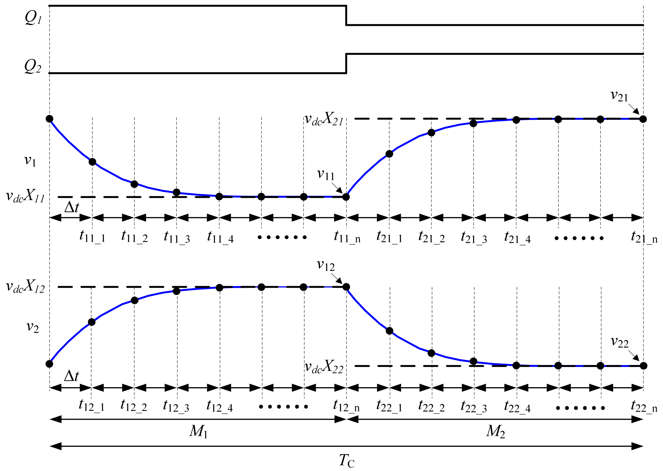
The traditional sampling method when GC exists is shown in Figure 3. In the M₁ phase, v₁ decreases slowly, and v₂ increases slowly. Sampling continues for v₁ and v₂ until t_{11_n} and t_{12_n}, respectively; v₁ falls to stable value v_dcX₁₁, and v₂ rises to stable value v_dcX₁₂. After stabilization, the final v₁₁ and v₁₂ are obtained. The method switches to the M₂ phase until v₁ and v₂ reach stable values v_dcX₂₁ and v_dcX₂₂, respectively, and the controller obtains the final v₂₁ and v₂₂. One sampling period T_C ends, and the insulation resistance values R_f2 and R_f1 are calculated by v₁₁ = v_dcX₁₁, v₁₂ = v_dcX₁₂, v₂₁ = v_dcX₂₁, and v₂₂ = v_dcX₂₂. The resistance values of R₁₁, R₁₂, R₂₁, and R₂₂ are large, so the charging time of the capacitor is long. Sampling and calculation should be performed after GC charging is completed; hence, the measurement time of the traditional method is long and unable to meet the real-time requirements of EVs. To avoid the measurement overtime caused by GC, a new insulation resistance monitoring method, namely, three-point climbing algorithm, is proposed.

Figure 4 shows that each phase is sampled three times, and the sampling intervals are equal. With v₁₁ as an example, the three sampling times are t_{11_1}, t_{11_2}, and t_{11_3}; the sampling voltage values are v_{11_1}, v_{11 _2}, and v_{11_3}, respectively, and the time intervals are Δt. Similar definitions of v₁₂, v₂₁, and v₂₂ are provided to facilitate the calculation, and E₁ and E₂ are used to present natural exponential function. The following equation is then obtained from (5).

$$\left\{\begin{array}{l}\frac{v_{11}{}_{\_1}-v_{11}{}_{\_2}}{v_{11}{}_{\_2}-v_{11}{}_{\_3}}=e^{-\frac{\Delta t}{{\tau }_1}}=E_1,\begin{array}{c}\\ \end{array}\frac{v_{12}{}_{\_1}-v_{12}{}_{\_2}}{v_{12}{}_{\_2}-v_{12}{}_{\_3}}=e^{-\frac{\Delta t}{{\tau }_1}}=E_1\\ \frac{v_{21}{}_{\_1}-v_{21}{}_{\_2}}{v_{21}{}_{\_2}-v_{21}{}_{\_3}}=e^{-\frac{\Delta t}{{\tau }_2}}=E_2,\begin{array}{c}\\ \end{array}\frac{v_{22}{}_{\_1}-v_{22}{}_{\_2}}{v_{22}{}_{\_2}-v_{22}{}_{\_3}}=e^{-\frac{\Delta t}{{\tau }_2}}=E_2\end{array}\right.$$

(6)

t_{11_1}, t_{12_1}, t_{21_1}, and t_{22_1} are set as initial times for the first-order circuit full response curve, and the curve Equation (5) is converted into Equation (7).

$$\left\{\begin{array}{l}{v}_{11}{}_{\_2}=v_{dc}{X}_{11}+(v_{11}{}_{\_1}-v_{dc}{X}_{11})E_1\\ v_{12}{}_{\_2}=v_{dc}{X}_{12}+(v_{12\_}{}_1-v_{dc}{X}_{12})E_1\\ v_{21}{}_{\_2}=v_{dc}{X}_{21}+(v_{21}{}_{\_1}-v_{dc}{X}_{21})E_2\\ v_{22}{}_{\_2}=v_{dc}{X}_{22}+(v_{22\_}{}_1-v_{dc}{X}_{22})E_2\end{array}\right.$$

(7)

Equation (7) is converted into Equation (8).

$$\left\{\begin{array}{l}{X}_{11}=\frac{v_{11}{}_{\_2}-v_{11}{}_{\_1}{E}_1}{v_{dc}(1-E_1)},\begin{array}{c}\\ \end{array}{X}_{12}=\frac{v_{12}{}_{\_2}-v_{12}{}_{\_1}{E}_1}{v_{dc}(1-E_1)}\\ X_{21}=\frac{v_{21}{}_{\_2}-v_{12}{}_{\_1}{E}_2}{v_{dc}(1-E_2)},\begin{array}{c}\\ \end{array}{X}_{22}=\frac{v_{22}{}_{\_2}-v_{22}{}_{\_1}{E}_2}{v_{dc}(1-E_2)}\end{array}\right.$$

(8)

X₁₁, X₁₂, X₂₁, and X₂₂ in Equation (8) are known values calculated by sampling voltage. Equation (9) can be obtained from Equations (2), (3), and (8), and insulation resistance values R_f1 and R_f2 can be solved.

$$\left\{\begin{array}{l}{R}_{f1}=\frac{R_a{R}_b}{\frac{R_a-R_b}{X_{12}-X_{22}}{X}_{12}-R_a},R_{f2}=\frac{R_a{R}_b}{\frac{R_b-R_a}{X_{11}-X_{21}}{X}_{11}-R_b}\\ R_{f1}=\frac{R_a{R}_b}{\frac{R_a-R_b}{X_{12}-X_{22}}{X}_{22}-R_b},R_{f2}=\frac{R_a{R}_b}{\frac{R_b-R_a}{X_{11}-X_{21}}{X}_{21}-R_a}\end{array}\right.$$

(9)

4. Implementation Method for Improving Accuracy

4.1. Error Analysis

In practical applications, sample resolution and voltage ripple cause sampling errors, which affect the calculated result of insulation resistance. With the v₁₁ of the M₁ phase as an example, Δv_{11_1}, Δv_{11_2}, and Δv_{11_3} are the sampling errors of v_{11_1}, v_{11_2}, and v_{11_3}, respectively. E_1R is the actual value of E₁. E_1C is the measured value of E₁. Considering the sampling error, the expression of E_1R and E_1C according to Equation (6) is shown as

$$\left\{\begin{array}{l}{E}_1{}_R=\frac{v_{11}{}_{\_2}-v_{11}{}_{\_3}}{v_{11}{}_{\_1}-v_{11}{}_{\_2}}\\ E_1{}_C=\frac{(v_{11}{}_{\_2}+\Delta v_{11}{}_{\_2})-(v_{11}{}_{\_3}+\Delta v_{11}{}_{\_3})}{(v_{11}{}_{\_1}+\Delta v_{11}{}_{\_1})-(v_{11}{}_{\_2}+\Delta v_{11}{}_{\_2})}\end{array}\right.$$

(10)

ΔE₁ is the error of $E_1$ and is defined as follows:

$$\Delta E_1=E_1{}_C-E_1{}_R$$

(11)

By substituting Equation (11) into Equation (10), ΔE₁ can be rewritten as

$$\Delta E_1=\frac{(\Delta v_{11}{}_{\_2}-\Delta v_{11}{}_{\_3})-E_1{}_R(\Delta v_{11}{}_{\_1}-\Delta v_{11}{}_{\_2})}{(v_{11}{}_{\_1}-v_{11}{}_{\_2})+(\Delta v_{11}{}_{\_1}-\Delta v_{11}{}_{\_2})}$$

(12)

where Δv_{11_1}, Δv_{11_2}, and Δv_{11_3} are uncontrollable components and E_1R is a fixed value. (v_{11_1–}v_{11_2}) is inversely proportional to ΔE₁. Similarly, v₁₂, v₂₁, and v₂₂ can result in the same conclusion. In the application, the larger Δt₁₁, Δt₁₂, Δt₂₁, and Δt₂₂ are, the smaller the result error is. The larger the difference between the R_a and R_b is, the smaller the result error is. The higher the v_dc is, the smaller the result error is.

4.2. Selection of Calculation Method

In the climbing stage, the smaller GC is, the larger the difference is in the three-point sampling and the smaller the result error is. If GC is too small, the sampling may reach the stable stage after climbing, the difference between the three sampled voltages will be too small, and the resulting error will increase. The accuracy is the highest only when the three sampled voltages are in the climbing stage of the voltage variation curve. Equation (6) shows that when the difference of the three sampled voltages is close to zero, the calculated value of ΔE₁ is nearly infinite because of signal interference in the actual application unlike in the ideal situation. This condition seriously affects the measurement result. A positive constant is set as C_a to determine if GC is too small by using the following rule.

$$\left\{\begin{array}{l}{v}_{11}{}_{\_2}-v_{11}{}_{\_3}<{\mathrm{C}}_{\mathrm{a}}\\ v_{22}{}_{\_2}-v_{22}{}_{\_3}<{\mathrm{C}}_{\mathrm{a}}\\ v_{12}{}_{\_2}-v_{12}{}_{\_3}>-{\mathrm{C}}_{\mathrm{a}}\\ v_{21}{}_{\_2}-v_{21}{}_{\_3}>-{\mathrm{C}}_{\mathrm{a}}\end{array}\right.$$

(13)

If the three sampled voltages satisfy Equation (13), then GC is too small to be non-negligible, and the traditional sampling method is adopted. If the three sampled voltages do not satisfy Equation (13), then GC is non-negligible, and the proposed three-point climbing algorithm is adopted.

4.3. Filter of E₁ and E₂

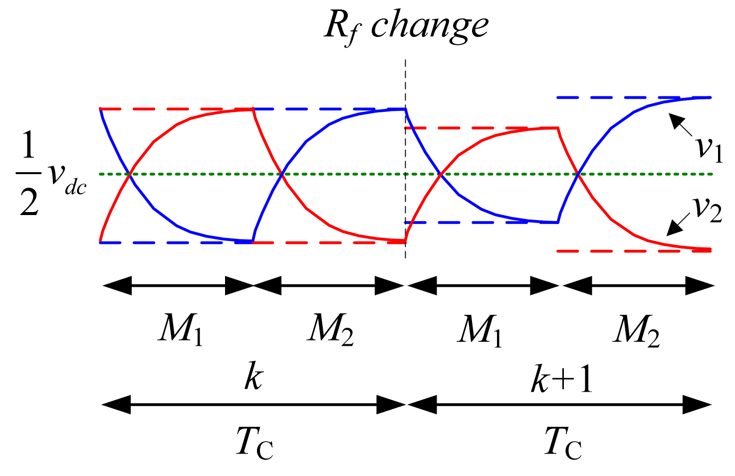
Δt is an invariant constant; ${\tau }_1$ and ${\tau }_2$ vary with GC, so E₁ and E₂ are also variations. Counter k is increased once every measurement period T_C, as shown in Figure 5. To make kth measurements E₁ and E₂ close to the actual value, the average value of M₁ and M₂ phases are taken according to Equation (6). E₁(k) and E₂(k) can be rewritten as

$$\left\{\begin{array}{l}{E}_1(k)=(\frac{v_{11}{}_{\_1}(k)-v_{11}{}_{\_2}(k)}{v_{11}{}_{\_2}(k)-v_{11}{}_{\_3}(k)}+\frac{v_{12}{}_{\_1}(k)-v_{12}{}_{\_2}(k)}{v_{12}{}_{\_2}(k)-v_{12}{}_{\_3}(k)})/2\\ E_2(k)=(\frac{v_{21}{}_{\_1}(k)-v_{21}{}_{\_2}(k)}{v_{21}{}_{\_2}(k)-v_{21}{}_{\_3}(k)}+\frac{v_{22}{}_{\_1}(k)-v_{22}{}_{\_2}(k)}{v_{22}{}_{\_2}(k)-v_{22}{}_{\_3}(k)})/2\end{array}\right.$$

(14)

The estimated value of the kth E₁ and E₂ is set as ${\widehat{E}}_1(k)$ and ${\widehat{E}}_2(k)$, respectively, which can be obtained by the following first-order filter, where A is a filter coefficient that satisfies 0 < A < 1.

$$\left\{\begin{array}{l}{\widehat{E}}_1(k)=\mathrm{A}{\widehat{E}}_1(k-1)+(1-\mathrm{A})E_1(k)\\ {\widehat{E}}_2(k)=\mathrm{A}{\widehat{E}}_2(k-1)+(1-\mathrm{A})E_2(k)\end{array}\right.$$

(15)

4.4. Correction of Sampled Value

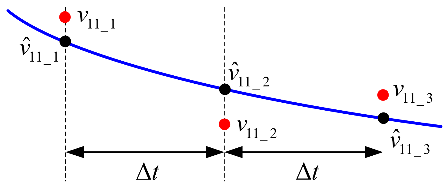
The actual sampled voltage value shows a certain deviation from the expected value. The red sampled point in Figure 6 shows that the exponential function curve cannot be formed. The result calculated by the sampled value must be a large error. Therefore, to obtain satisfactory results, the sampled values must be corrected with a loop iterative correction method. ${\widehat{v}}_{11\_1}(i)$,${\widehat{v}}_{11\_2}(i)$,${\widehat{v}}_{11\_3}(i)$,${\widehat{v}}_{12\_1}(i)$,${\widehat{v}}_{12\_2}(i)$,${\widehat{v}}_{12\_3}(i)$,${\widehat{v}}_{21\_1}(i)$,${\widehat{v}}_{21\_2}(i)$,${\widehat{v}}_{21\_3}(i)$,${\widehat{v}}_{22\_1}(i)$,${\widehat{v}}_{22\_2}(i)$, and ${\tilde{v}}_{22\_3}(i)$ are set as the ith correction voltage values. After the 12 voltages of v₁₁, v₁₂, v₂₁, and v₂₂ are sampled completely, the counter is set as i = 0. The 12 voltage values are substituted into the following equation, and the sampled value is used as the initial correction value.

$$\left\{\begin{array}{l}{\widehat{v}}_{11\_1}(0)=v_{11}{}_{\_1}\\ {\widehat{v}}_{11\_2}(0)=v_{11}{}_{\_2}\\ {\widehat{v}}_{11\_3}(0)=v_{11}{}_{\_3}\end{array}\right.,\left\{\begin{array}{l}{\widehat{v}}_{12\_1}(0)=v_{12}{}_{\_1}\\ {\widehat{v}}_{12\_2}(0)=v_{12}{}_{\_2}\\ {\widehat{v}}_{12\_3}(0)=v_{12}{}_{\_3}\end{array}\right.\left\{\begin{array}{l}{\widehat{v}}_{21\_1}(0)=v_{21}{}_{\_1}\\ {\widehat{v}}_{21\_2}(0)=v_{21}{}_{\_2}\\ {\widehat{v}}_{21\_3}(0)=v_{21}{}_{\_3}\end{array}\right.,\left\{\begin{array}{l}{\widehat{v}}_{22\_1}(0)=v_{22}{}_{\_1}\\ {\widehat{v}}_{22\_2}(0)=v_{22}{}_{\_2}\\ {\widehat{v}}_{22\_3}(0)=v_{22}{}_{\_3}\end{array}\right.$$

(16)

The three sampled voltages of each group cannot form an exponential curve of ${\widehat{E}}_1(k)$ due to the measurement error and ripple. To form the desired exponential curve, each voltage value can be estimated by the two other voltage values. ${\tilde{v}}_{11\_1}(i)$,${\tilde{v}}_{11\_2}(i)$,${\tilde{v}}_{11\_3}(i)$,${\tilde{v}}_{12\_1}(i)$,${\tilde{v}}_{12\_2}(i)$,${\tilde{v}}_{12\_3}(i)$,${\tilde{v}}_{21\_1}(i)$,${\tilde{v}}_{21\_2}(i)$,${\tilde{v}}_{21\_3}(i)$,${\tilde{v}}_{22\_1}(i)$,${\tilde{v}}_{22\_2}(i)$, and ${\tilde{v}}_{22\_3}(i)$ are set as the estimated voltage values. The estimated method can be derived from the following equation according to Equation (6).

$$\begin{array}{l}\{\begin{array}{l}{\tilde{v}}_{11\_1}(i)=[{\widehat{v}}_{11\_2}(i)-{\widehat{v}}_{11\_3}(i)]{\widehat{E}}_1{(k)}^{-1}+{\widehat{v}}_{11\_2}(i)\\ {\tilde{v}}_{11\_2}(i)=[{\widehat{v}}_{11\_1}(i){\widehat{E}}_1(k)+{\widehat{v}}_{11\_3}(i)]/(1+{\widehat{E}}_1(k))\\ {\tilde{v}}_{11\_3}(i)={\widehat{v}}_{11\_2}(i)-[{\widehat{v}}_{11\_1}(i)-{\widehat{v}}_{11\_2}(i)]{\widehat{E}}_1(k)\end{array},\{\begin{array}{l}{\tilde{v}}_{12\_1}(i)=[{\widehat{v}}_{12\_2}(i)-{\widehat{v}}_{12\_3}(i)]{\widehat{E}}_1{(k)}^{-1}+{\widehat{v}}_{12\_2}(i)\\ {\tilde{v}}_{12\_2}(i)=[{\widehat{v}}_{12\_1}(i){\widehat{E}}_1(k)+{\widehat{v}}_{12\_3}(i)]/(1+{\widehat{E}}_1(k))\\ {\tilde{v}}_{12\_3}(i)={\widehat{v}}_{12\_2}(i)-[{\widehat{v}}_{12\_1}(i)-{\widehat{v}}_{12\_2}(i)]{\widehat{E}}_1(k)\end{array}\\ \{\begin{array}{l}{\tilde{v}}_{21\_1}(i)=[{\widehat{v}}_{21\_2}(i)-{\widehat{v}}_{21\_3}(i)]{\widehat{E}}_2{(k)}^{-1}+{\widehat{v}}_{21\_2}(i)\\ {\tilde{v}}_{21\_2}(i)=[{\widehat{v}}_{21\_1}(i){\widehat{E}}_2(k)+{\widehat{v}}_{21\_3}(i)]/(1+{\widehat{E}}_2(k))\\ {\tilde{v}}_{21\_3}(i)={\widehat{v}}_{21\_2}(i)-[{\widehat{v}}_{21\_1}(i)-{\widehat{v}}_{21\_2}(i)]{\widehat{E}}_2(k)\end{array},\{\begin{array}{l}{\tilde{v}}_{22\_1}(i)=[{\widehat{v}}_{22\_2}(i)-{\widehat{v}}_{22\_3}(i)]{\widehat{E}}_2{(k)}^{-1}+{\widehat{v}}_{22\_2}(i)\\ {\tilde{v}}_{22\_2}(i)=[{\widehat{v}}_{22\_1}(i){\widehat{E}}_2(k)+{\widehat{v}}_{22\_3}(i)]/(1+{\widehat{E}}_2(k))\\ {\tilde{v}}_{22\_3}(i)={\widehat{v}}_{22\_2}(i)-[{\widehat{v}}_{22\_1}(i)-{\widehat{v}}_{22\_2}(i)]{\widehat{E}}_2(k)\end{array}\end{array}$$

(17)

The estimated value comparison rule is shown as

$$\begin{array}{l}\{\begin{array}{l}\left|{\widehat{v}}_{11\_1}(i)-{\tilde{v}}_{11\_1}(i)\right|<\mathrm{D},\left|{\widehat{v}}_{11\_2}(i)-{\tilde{v}}_{11\_2}(i)\right|<\mathrm{D},\left|{\widehat{v}}_{11\_3}(i)-{\tilde{v}}_{11\_3}(i)\right|<\mathrm{D}\\ \left|{\widehat{v}}_{12\_1}(i)-{\tilde{v}}_{12\_1}(i)\right|<\mathrm{D},\left|{\widehat{v}}_{12\_2}(i)-{\tilde{v}}_{12\_2}(i)\right|<\mathrm{D},\left|{\widehat{v}}_{12\_3}(i)-{\tilde{v}}_{12\_3}(i)\right|<\mathrm{D}\end{array}\\ \{\begin{array}{l}\left|{\widehat{v}}_{21\_1}(i)-{\tilde{v}}_{21\_1}(i)\right|<\mathrm{D},\left|{\widehat{v}}_{21\_2}(i)-{\tilde{v}}_{21\_2}(i)\right|<\mathrm{D},\left|{\widehat{v}}_{21\_3}(i)-{\tilde{v}}_{21\_3}(i)\right|<\mathrm{D}\\ \left|{\widehat{v}}_{22\_1}(i)-{\tilde{v}}_{22\_1}(i)\right|<\mathrm{D},\left|{\widehat{v}}_{22\_2}(i)-{\tilde{v}}_{22\_2}(i)\right|<\mathrm{D},\left|{\widehat{v}}_{22\_3}(i)-{\tilde{v}}_{22\_3}(i)\right|<\mathrm{D}\end{array}\end{array}$$

(18)

When Equation (18) is satisfied, the difference between the estimated value and the correction value is small, and the ith correction value is applied as the final correction value. Otherwise, the counter i is increased by 1, and further correction is be conducted as follows:

$$\begin{array}{l}\{\begin{array}{l}{\widehat{v}}_{11\_1}(i+1)={\tilde{v}}_{11\_1}(i)+\mathrm{B}[{\widehat{v}}_{11\_1}(i)-{\tilde{v}}_{11\_1}(i)]\\ {\widehat{v}}_{11\_2}(i+1)={\tilde{v}}_{11\_2}(i)+\mathrm{B}[{\widehat{v}}_{11\_2}(i)-{\tilde{v}}_{11\_2}(i)]\\ {\widehat{v}}_{11\_3}(i+1)={\tilde{v}}_{11\_3}(i)+\mathrm{B}[{\widehat{v}}_{11\_3}(i)-{\tilde{v}}_{11\_3}(i)]\end{array},\{\begin{array}{l}{\widehat{v}}_{12\_1}(i+1)={\tilde{v}}_{12\_1}(i)+\mathrm{B}[{\widehat{v}}_{12\_1}(i)-{\tilde{v}}_{12\_1}(i)]\\ {\widehat{v}}_{12\_2}(i+1)={\tilde{v}}_{12\_2}(i)+\mathrm{B}[{\widehat{v}}_{12\_2}(i)-{\tilde{v}}_{12\_2}(i)]\\ {\widehat{v}}_{12\_3}(i+1)={\tilde{v}}_{12\_3}(i)+\mathrm{B}[{\widehat{v}}_{12\_3}(i)-{\tilde{v}}_{12\_3}(i)]\end{array}\\ \{\begin{array}{l}{\widehat{v}}_{21\_1}(i+1)={\tilde{v}}_{21\_1}(i)+\mathrm{B}[{\widehat{v}}_{21\_1}(i)-{\tilde{v}}_{21\_1}(i)]\\ {\widehat{v}}_{21\_2}(i+1)={\tilde{v}}_{21\_2}(i)+\mathrm{B}[{\widehat{v}}_{21\_2}(i)-{\tilde{v}}_{21\_2}(i)]\\ {\widehat{v}}_{21\_3}(i+1)={\tilde{v}}_{21\_3}(i)+\mathrm{B}[{\widehat{v}}_{21\_3}(i)-{\tilde{v}}_{21\_3}(i)]\end{array},\{\begin{array}{l}{\widehat{v}}_{22\_1}(i+1)={\tilde{v}}_{22\_1}(i)+\mathrm{B}[{\widehat{v}}_{22\_1}(i)-{\tilde{v}}_{22\_1}(i)]\\ {\widehat{v}}_{22\_2}(i+1)={\tilde{v}}_{22\_2}(i)+\mathrm{B}[{\widehat{v}}_{22\_2}(i)-{\tilde{v}}_{22\_2}(i)]\\ {\widehat{v}}_{22\_3}(i+1)={\tilde{v}}_{22\_3}(i)+\mathrm{B}[{\widehat{v}}_{22\_3}(i)-{\tilde{v}}_{22\_3}(i)]\end{array}\end{array}$$

(19)

where B is the correction factor that satisfies 0 < B < 1. Then, the results of Equation (19) are substituted into Equation (17). This method cycles back and forth until the difference between the estimated and correction values satisfies Equation (18). The cycle is then stopped, and the final correction value is outputted.

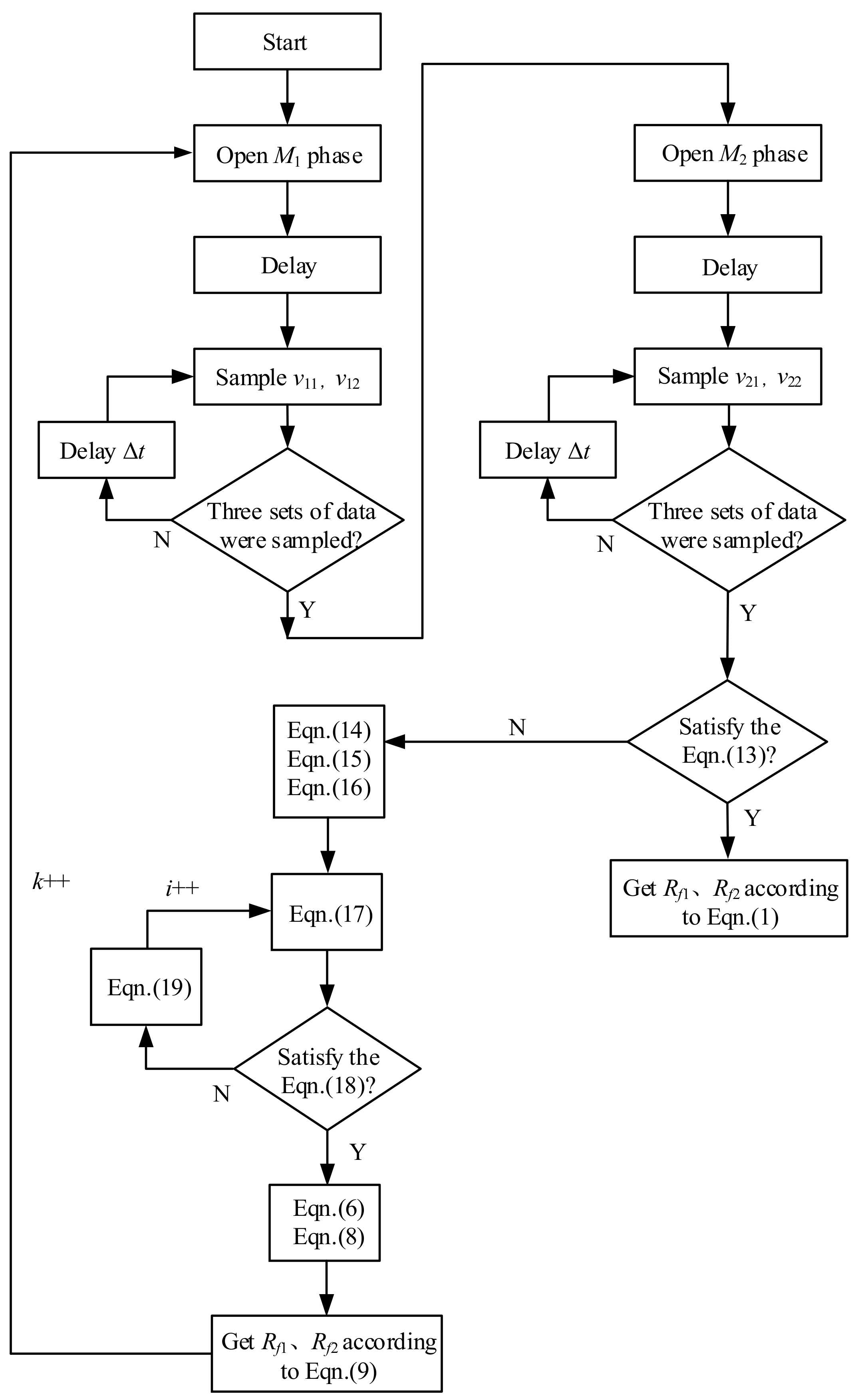
The overall software flow chart of the method is shown in Figure 7.

5. Comparative Study of Experimental Data

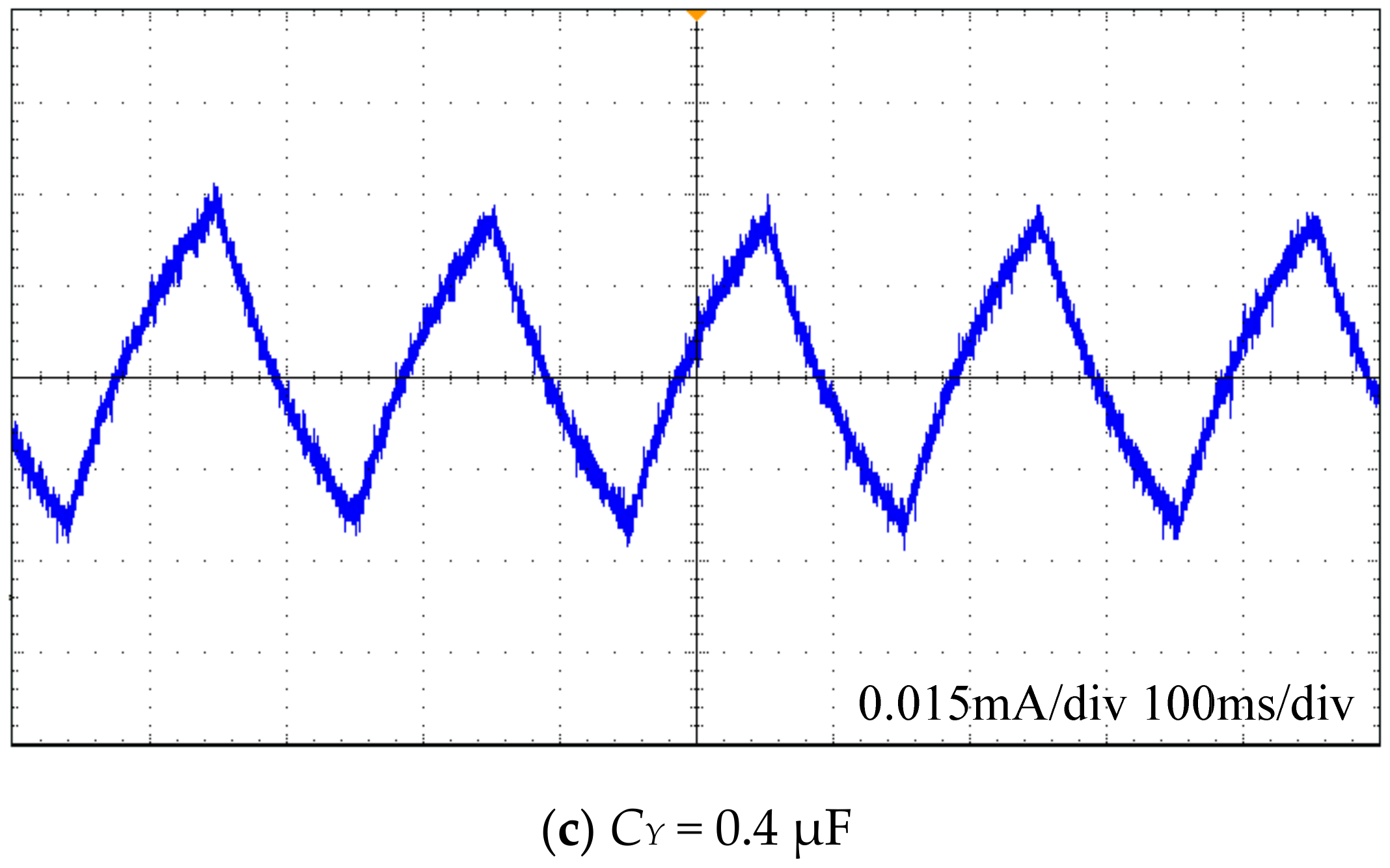
The DC-IM device with the unbalanced electric bridge method is created, and the schematic overview of application is shown in Figure 8. The MCU performs the switch Q₁ and Q₂, sample the voltage values of v₁ and v₂ stored in memory, then calculate the R_f1 and R_f2, and output the result to the computer. The experiment table is shown in Figure 9. It includes the display interface, DC-IM device, voltage regulating device, insulation resistance selection switch, and GC selection switch. The DC-IM controller uses a PIC18F4580 single-chip microcomputer. The monitoring period is 0.2 s; that is, the switch action occurs every 0.1 s, so the sampling time should satisfy (t₁ + 2Δt) < 0.1 s. The positive grounding resistance is R_f1 = 1000 kΩ, the negative grounding resistance is R_f2 = 300 kΩ, the first sampling time t₁ = 0.01 s, the bridge resistance is R_a = 1000 kΩ, and R_b = 200 kΩ. The GC value is C_Y = C₁ = C₂. The grounding current waveform corresponding to different GCs is shown in Figure 10. The waveform of C_Y = 0.1 μF can be stabilized in a half cycle. The larger the value of C_Y is, the closer the waveform is to the triangle wave. Therefore, the traditional unbalanced bridge sampling method is used when C_Y < 0.1 μF, and the three-point climbing algorithm is used when C_Y > 0.1 μF.

The calculation results are compared by changing the different parameters, and relative error (RE%) is determined as

RE% = | measured value − actual value |/measured value.

(20)

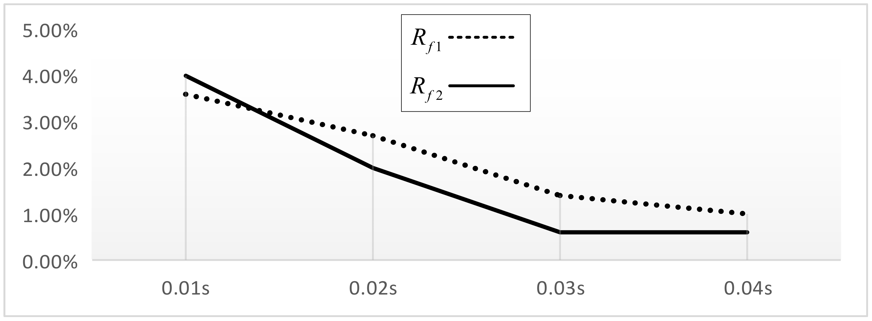
Different parameters are applied in the proposed method. (1) DC voltage v_dc = 800 V, GC value C_Y = 0.1 μF, and the sampling time interval Δt is changed; the results are shown in Figure 11. The larger the sampling time interval is, the higher accuracy is. (2) DC voltage v_dc = 800 V, sampling time interval Δt = 0.04 s, and the value of C_Y is changed; the results are shown in Figure 12. The smaller C_Y is, the higher accuracy is. (3) Sampling interval Δt = 0.04 s, C_Y = 0.1 μF, and DC voltage v_dc is changed; the results are shown in Figure 13. The larger the DC voltage is, the higher accuracy is. When the DC voltage drops to below 200 V, the measurement accuracy is greatly reduced. (4) Under the premise that the parallel value of bridge resistance R_a || R_b is constant and the difference between R_a and R_b is changed; the results are shown in

Table 2. Data results with different bridge resistors.

Ra (kΩ)	Rb (kΩ)	Rf1 (kΩ)	RE% of Rf1	Rf2 (kΩ)	RE% of Rf2
1000	200	1010	1.0%	302	0.6%
800	250	1014	1.4%	305	1.6%
600	300	1020	2.0%	309	3.0%
500	350	1045	4.5%	316	5.3%

. The larger the difference between R_a and R_b is, the higher accuracy is. Time interval Δt increases, C_Y decreases, DC voltage v_dc increases, and the difference between R_a and R_b increases. These factors make the sampled voltage difference larger, which will reduce the error of the final results.

The proposed method is compared with the traditional method to verify the availability and superiority of the former. The monitoring time and relative error of the two methods are shown in

Table 3. Comparison of monitoring data in v_dc = 800 V, R_f1 = 1000 kΩ, R_f2 = 300 kΩ.

	Traditional Method		Proposed Method
CY	Monitoring Time	RE%	Monitoring Time	RE%
10 nF	0.2s	0.8%	0.2s	0.8%
0.1 μF	0.3s	1.0%	0.2s	1.2%
1 μF	1.35s	2.4%	0.2s	1.8%
2 μF	2.51s	3.5%	0.2s	3.7%
3 μF	3.67s	5%	0.2s	5.3%
4 μF	4.83s	6.6%	0.2s	7.3%

,

Table 4. Comparison of monitoring data in v_dc = 400 V, R_f1 = 1000 kΩ, R_f2 = 300 kΩ.

	Traditional Method		Proposed Method
CY	Monitoring Time	RE%	Monitoring Time	RE%
10 nF	0.2s	1.3%	0.2s	1.3%
0.1 μF	0.29s	1.7%	0.2s	2.8%
1 μF	0.34s	3.2%	0.2s	4.1%
2 μF	2.49s	5.8%	0.2s	6.2%
3 μF	3.64s	8.5%	0.2s	9%
4 μF	4.79s	11%	0.2s	12%

and

Table 5. Comparison of monitoring data in v_dc = 800 V, R_f1 = 100 kΩ, R_f2 = 100 kΩ.

	Traditional Method		Proposed Method
CY	Monitoring Time	RE%	Monitoring Time	RE%
10 nF	0.2s	0.7%	0.2s	0.7%
0.1 μF	0.23s	1.0%	0.2s	0.9%
1 μF	0.65s	2.2%	0.2s	1.6%
2 μF	1.11s	3.4%	0.2s	2.4%
3 μF	1.57s	4.7%	0.2s	4.1%
4 μF	2s	6.3%	0.2s	5.2%

. The relative error is the larger one between R_f1 and R_f2. Table 3 is the data at v_dc = 800 V, R_f1 = 1000 kΩ, R_f2 = 300 kΩ; Table 4 is the data at v_dc = 400 V, R_f1 = 1000 kΩ, R_f2 = 300 kΩ; Table 5 is the data at v_dc = 800 V, R_f1 = 100 kΩ, R_f2 = 100 kΩ. The traditional method needs to increase the monitoring time with a large value of GC because it should have a stable sample value after charging the GC. The proposed method has a fixed monitoring time due to the fixed three-point sampling. When GC is large and the proposed method is applied, the error is similar to using the traditional method. When GC is small, such as 10 nF in the table, and the traditional unbalanced bridge calculation method is applied automatically, the calculation results of two methods are almost the same. Overall, the experimental results are consistent with the theoretical conclusion.

6. Conclusions

For the DC-IM circuit of EVs, the traditional unbalanced electric bridge method switches the positive and negative bridge resistances and calculates the insulation resistance value by sampling the positive and negative bridge voltages. However, when the DC positive and negative poles have GC, the bridge voltages must be sampled after the capacitor is charged completely; thus, the measurement time is very long. This study proposes a novel method of DC-IM using a three-point climbing algorithm. The insulation resistance can be calculated by sampling the voltage of the positive and negative bridges three times and keeping the sampling interval equal. Moreover, the method filters and automatically corrects the three sampling voltages, which can improve the accuracy of the calculation results. Combined with experimental data, the following conclusions can be drawn: (1) The advantage of proposed method can perform a faster time and maintain a constant monitoring period compared with the traditional method. (2) The restriction of proposed method only apply in larger GC situation. If GC is small, the traditional method could be used. (3) The characteristics of proposed method: Increasing the sampling interval, increasing the difference between R_a and R_b, increasing DC voltage v_dc, all make the results more accurate. Overall, the proposed method can be applied to some practical industrial applications. The future work is to study how to set the constant C_a to determine which method to use or find a different rule to generally judge the value of GC, and study a method to reduce error when v_dc is constant changing.

References

- Hou, Y.P.; Zhou, W.; Shen, C.Y. Experimental investigation of gas-tightness and electrical insulation of fuel cell stack under strengthened road vibrating conditions. Int. J. Hydrogen Energy 2011, 36, 13763–13768. [Google Scholar] [CrossRef]
- Gyftakis, K.N.; Sumislawska, M.; Kavanagh, D.F.; Howey, D.A.; McCulloch, M.D. Dielectric Characteristics of Electric Vehicle Traction Motor Winding Insulation Under Thermal Aging. IEEE Trans. Ind. Appl. 2016, 52, 1398–1404. [Google Scholar]
- Dannier, A. Overview of Main Electric Subsystems of Zero-Emission Vehicles. Propuls. Syst. 2019, 1–31. [Google Scholar] [CrossRef]
- Vahedipour-Dahraie, M.; Rashidizaheh-Kermani, H.; Najafi, H.R.; Anvari-Moghaddam, A.; Guerrero, J.M. Coordination of EVs Participation for Load Frequency Control in Isolated Microgrids. Appl. Sci. 2017, 7, 539. [Google Scholar] [CrossRef]
- Rafique, M.K.; Khan, S.U.; Zaman, M.S.U.; Mehmood, K.K.; Haider, Z.M.; Ali Bukhar, S.B.; Kim, C. An Intelligent Hybrid Energy Management System for a Smart House Considering Bidirectional Power Flow and Various EV Charging Techniques. Appl. Sci. 2019, 9, 1658. [Google Scholar] [CrossRef]
- Kim, J.; Kim, H.; Cho, Y.; Kim, H.; Cho, J. Application of a DC Distribution System in Korea: A Case Study of the LVDC Project. Appl. Sci. 2019, 9, 1074. [Google Scholar] [CrossRef]
- Holger Potdevin, D.-I. Insulation Monitoring in High Voltage Systems for Hybrid and Electric Vehicles. High Voltage Safety. ATZ Elektron. 2009, 4, 28–31. [Google Scholar] [CrossRef]
- Pan, X.F.; Rinkleff, T.; Willmann, B.; Vick, R. PSpice simulation of surge testing for electrical vehicles. In Proceedings of the 2012 International Symposium on Electromagnetic Compatibility (EMC EUROPE), Rome, Italy, 17–21 September 2012. [Google Scholar]
- Liu, Y.-C.; Lin, C.-Y. Insulation fault detection circuit for ungrounded DC power supply systems. In Proceedings of the 2012 IEEE Sensors, Taipei, Taiwan, 28–31 October 2012. [Google Scholar]
- Zhao, C.Y.; Jia, X.F.; Hao, Z.F. The new method of monitoring DC system insulation on-line. In Proceedings of the 27th Annual Conference of the IEEE Industrial Electronics Society, IECON’01, Denver, CO, USA, 29 November–2 December 2001. [Google Scholar]
- Jiang, J.S.; Ji, H. Study of Insulation Monitoring Device for DC System Based on Multi-switch Combination. In Proceedings of the Second International Symposium on Computational Intelligence and Design, ISCID’09, Changsha, China, 12–14 December 2009. [Google Scholar]
- Li, J.X.; Wu, Z.Q.; Fan, Y.Q.; Wang, Y.Y.; Jiang, J.C. Research on Insulation Resistance On-Line Monitoring for Electric Vehicle. In Proceedings of the 2005 International Conference on Electrical Machines and Systems, Nanjing, China, 27–29 September 2005. [Google Scholar]
- Wei, X.Y.; Bi, L.; Sun, Z.C. A method of insulation failure detection on electric vehicle based on FPGA. In Proceedings of the 2008 IEEE Vehicle Power and Propulsion Conference, VPPC’08, Harbin, China, 3–5 September 2008. [Google Scholar]
- Zheng, M.X. The Design of Insulation Monitoring Device for Electric Vehicle’s Battery Pack. Adv. Mater. Res. 2013, 718–720, 1422–1428. [Google Scholar] [CrossRef]
- Bao, Y.; Jiang, J.C.; Zhang, W.G.; Wang, J.Y.; Wen, J.P. Novel On-line Insulation Supervising Method for DC System. High Volt. Eng. 2011, 37, 333–337. [Google Scholar]
- Wu, Z.J.; Wang, L.F. A novel insulation resistance monitoring device for Hybrid Electric Vehicle. In Proceedings of the 2008 IEEE Vehicle Power and Propulsion Conference, VPPC’08, Harbin, China, 3–5 September 2008. [Google Scholar]
- Neti, P.; Grubic, S. Online broadband insulation spectroscopy of induction machines using signal injection. IEEE Trans. Ind. Appl. 2017, 53, 1054–1062. [Google Scholar] [CrossRef]
- Chiang, Y.-H.; Sean, W.-Y.; Huang, C.-Y.; Chiang Hsieh, L.-H. Adaptive control for estimating insulation resistance of high-voltage battery system in electric vehicles. Environ. Prog. Sustain. Energy 2017, 36, 1882–1887. [Google Scholar] [CrossRef] [Green Version]
- Li, D.H.; Jia, W. Application of Chaos Theory in Grounaing Fault Detection of DC Power Supply System. High Volt. Eng. 2005, 31, 79–82. [Google Scholar]
- Li, D.H.; Shi, L.T. An Overall Scheme for Ground Fault Detection in DC Systems of Power Plants and Substations. Power Syst. Technol. 2005, 29, 56–59. [Google Scholar]
- Song, C.X.; Shao, Y.L.; Song, S.X.; Peng, S.L.; Zhou, F.; Chang, C.; Wang, D. Insulation Resistance Monitoring Algorithm for Battery Pack in Electric Vehicle Based on Extended Kalman Filtering. Energies 2017, 10, 714. [Google Scholar] [CrossRef]
Figure 1.
The circuit of unbalanced bridge. (a) The circuit of M1 phase. (b) The circuit of M2 phase. (c) The equivalent circuit of M1 phase. (d) The equivalent circuit of M2 phase.
Figure 2.
Equivalent circuit of unbalanced bridge with GC. (a) The circuit of M1 phase. (b) The circuit of M2 phase. (c) The equivalent circuit of M1 phase. (d) The equivalent circuit of M2 phase.
Figure 3.
Traditional sampling method.
Figure 4.
Proposed three-point climbing algorithm.
Figure 5.
Waveform of the bridge voltage.
Figure 6.
Actual sampling point.
Figure 7.
Software flow chart of the proposed method.
Figure 8.
The schematic overview of application.
Figure 9.
Display of the experiment table.
Figure 10.
Waveform of grounding current with different values of CY. (a) CY = 0.1 μF. (b) CY = 0.2 μ. (c) CY = 0.4 μF.
Figure 11.
RE% with different sampling intervals.
Figure 12.
RE% with different values of CY.
Figure 13.
RE% with different DC voltages.