Modeling of CO Emissions from Traffic Vehicles Using Artificial Neural Networks

Abstract

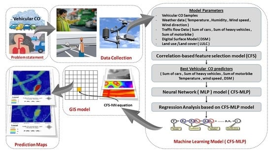
Traffic emissions are considered one of the leading causes of environmental impact in megacities and their dangerous effects on human health. This paper presents a hybrid model based on data mining and GIS models designed to predict vehicular Carbon Monoxide (CO) emitted from traffic on the New Klang Valley Expressway, Malaysia. The hybrid model was developed based on the integration of GIS and the optimized Artificial Neural Network algorithm that combined with the Correlation based Feature Selection (CFS) algorithm to predict the daily vehicular CO emissions and generate prediction maps at a microscale level in a small urban area by using a field survey and open source data, which are the main contributions to this paper. The other contribution is related to the case study, which represents the spatial and quantitative variations in the vehicular CO emissions between toll plaza areas and road networks. The proposed hybrid model consists of three steps: the first step is the implementation of the correlation-based Feature Selection model to select the best model’s predictors; the second step is the prediction of vehicular CO by using a multilayer perceptron neural network model; and the third step is the creation of micro scale prediction maps. The model was developed using six traffic CO predictors: number of vehicles, number of heavy vehicles, number of motorbikes, temperature, wind speed and a digital surface model. The network architecture and its hyperparameters were optimized through a grid search approach. The traffic CO concentrations were observed at 15-min intervals on weekends and weekdays, four times per day. The results showed that the developed model had achieved validation accuracy of 80.6 %. Overall, the developed models are found to be promising tools for vehicular CO simulations in highly congested areas.

1. Introduction

The transport infrastructure like expressways and roads has a significant importance in the development of any country’s economy by linking cities. These infrastructures are rapidly developing due to the changing in the traffic modes, leading to congested roads. Hence, road traffic emissions are increasing, creating many negative impacts on air quality on roadways, intersections and toll roads. Traffic emissions, such as carbon monoxide (CO), are the primary contributor to overall air pollution from this infrastructure, and the primary source of traffic emissions is vehicular exhausts.

Spatial prediction models are effectively used as a decision-making support tool for prediction and simulation of traffic emissions on road networks [1,2,3]. There are various negative impacts that can result from inappropriate traffic levels, including high levels of noise and high concentrations of gaseous pollutants [4,5]. Several diseases e.g., cancers, heart diseases, respiratory problems and preterm births, can occur when human beings are exposed to high concentrations of CO [6,7,8].

The measurement of vehicular emissions on roadways and toll gates may be costly, risky and requires a lot of time and effort. Moreover, the designers do not have the opportunity to determine the vehicular emissions through the design process. In the most recent planning techniques for design of highways and road networks, traffic emission models are often required to support sustainable transportation planning and the reduction of traffic emissions from sources such as congestion and tollgate areas. Thus, the GIS-based modeling of traffic emission and intra-urban air pollution exposure can be an effective tool in the environmental assessment for sustainable road planning. This tool can distinguish the areas affected by different types of pollutants and the related ecological and social factors. This would be able to determine the best strategy to support the decision makers [9]. On the other hand, GIS can save costs and time in the traffic emission modeling and can therefore be used in sustainable planning.

Different types of traffic CO prediction approaches are mentioned in the literature [10,11,12]. Early methods of traffic CO modelling were based on traditional techniques using data sampling and global position system (GPS) techniques. Several thematic maps and vehicle emission equations are combined to model the traffic emission distribution in a region and produce informative maps that could help in effective decision making [10]. Recent methods are mostly based on land-use regression analysis using statistical and soft computing algorithms [10,13]. These statistical and computing techniques allow the input of various traffic and road geometry factors. Almost all these models are designed by using experimental samples; consequently, these models are highly influenced by the traffic flow condition and the measurement style and the geographic locations [14]. The main drawback of these models is that they can not be generalized because of the local environment like vehicle model and type and the weather [15,16]. Ref. [17] presented an approach of recognizing the road geometric features from positioning information surveyed by collecting vehicle data.

2. Previous Works

Many models have been developed to predict CO emissions and other traffic emissions, such as NOx, NO₂, CO₂ and SO₂. In a paper, Ref. [18] presented a methodology by integrating the spatial analysis techniques and the neighborhood statistic function algorithm to evaluate the spatial diffusion of the gaseous pollutant in north of Italy by using the air pollutant records obtained from monitoring stations and GIS data (i.e., administrative borders, built-up areas, emission sources and road networks). Their results were illustrated on grids with a cell size of (4 × 4) km. Although this method showed a significant spatial representation of air pollution, the methodology was constrained by the limited spatial resolution. Therefore, it cannot be used for high-resolution data. Ref. [19] developed a GIS-based tool by combining the operational street pollution model (OSPM) and a multi-agent-based transportation model (MATSIM) to estimate the air pollutant concentrations in Munich, Germany. Their results showed hourly prediction of NOx from traffic. This approach can be used as an effective tool for air quality studies in urban areas. Nevertheless, its disadvantages appear in the complexity of a system that comprises different models where the non-expert users are not able to use it. Ref. [20] developed a model based on land-use regression algorithm and land-use types, meteorological variables and vehicle-kilometers-travelled (VKTs) and linear regression algorithm to estimate the concentrations of Nitrogen Dioxide (NO₂) in Seoul, Korea. The results showed the significant impacts of the residential, commercial land use, wind speed, temperature and humidity on the concentrations of NO₂. The air pollutants recorded by the fixed air quality monitoring stations can be affected by several factors such as terrain and buildings altitude. Moreover, the weather factors are not suitable to model and produce high-resolution products such as roadmaps. Ref. [21] presented a statistical model based on the fuzzy logic system to predict CO concentrations in Tehran, Iran. This model mainly relied on historical data, which were obtained from monitoring stations. Fuzzy logic algorithms were applied to combine the parameters. Their results showed that lowest Room Mean Square Error (RMSE) was recorded at 2.13. Another study related to statistical modeling was conducted by [22] to forecast air pollutants in Hong Kong based on the integration of two statistical models, i.e., the generalized additive models and the Global Forecast System, which linked the air pollution with meteorological data. Results showed a contrast in the air pollutant levels between urban and suburban areas. This model is useful for predicting air quality in complex terrain areas. These models lack the spatial aspect and could not be used to produce prediction maps. Ref. [23] developed a methodology by using two commercial programs to estimate the traffic emissions in small area in Madrid, Spain. The VISSIM program was used for traffic simulation to calculate a velocity-time profile. Then, the related emissions at the vehicle level were completed using the VERSIT + micro program. Results showed the spatial variation in NOx and PM₁₀ concentrations are based on microscale maps with high resolution, cell size (5 × 5) m. This model depends on the estimated emissions data based on prediction simulations without using actual samples based on sampling equipment.

Recently, machine-learning technologies have attracted researchers. The neural network (NN) models are the most popular models in the Artificial Intelligence models. Ref. [24] developed a model by integrating the artificial neural network (ANN) algorithm and evolutionary polynomial regression (EPR) to estimate the CO concentrations in Tabriz City, Iran. The EPR is one of the data mining algorithms developed based on evolutionary computing and the integration of numerical regression and genetic algorithm. The EPR model involves two stages: a genetic algorithm is used in the first stage based on the numerical regression to search for symbolic structures, whereas in the second stage, symbolic structure parameters are determined based on the linear least squares techniques. Their results showed that the ANN model is more reliable than the EPR model. The highest value of the correlation coefficient was measured at 0.85 based on NN and 0.41 using EPR. This study indicated that NN modeling can be efficiently utilized for air quality forecasting. On the other hand, ref. [25] developed a model based on the NN algorithm and data obtained from field survey to estimate the hourly traffic emissions near roads. The authors used different parameters such as traffic data, meteorology, proximity to roads and road direction. This model is considered as an efficient approach for predicting pollutant near a road. Although they used geographic information as a parameter, their results did not contain spatial prediction results such as maps. They only presented a statistical analysis. Results showed that the highest correlation coefficient for the CO prediction was 0.879. Ref. [26] conducted the most relevant studies that combined the NN model and the spatial prediction model. They presented an approach that combined the linear-chain conditional random field algorithm and ANN model to generate real-time air pollution maps. They utilized the data recorded from monitoring stations and the traffic data collected from the field while geographic parameters like land use and road network were derived using GIS data. Their results showed the air pollutants prediction on maps with (1 × 1) km spatial resolution. However, the developed model did not consider many issues like uncertainty, modeling multifactor and nonlinearity. Although several authors have attempted to overcome these issues, they principally focused on the integration of big data and the large scale modeling. On the other hand, most of these models deal with large quantities of data, expensive equipment, and complex data processing models, which require substantial time, cost and other resources.

In this paper, we presented a hybrid model to produce microscale prediction maps considering toll gate locations, as well as the other parameters listed in the literature. The model is developed by combining the metaheuristic optimization technique and ANN algorithm to predict traffic emissions based on a small number of training data and avoiding transferability issues. The metaheuristic optimization algorithms like correlation-based feature selection models which have the ability to find best model’s predictors in a short time were compared to other optimization techniques. Also, ANN algorithms are suitable for prediction based on few training data. The major contributions of this work lie in producing highly accurate predictive maps and providing a description of the high variation of traffic emissions on roads and tollgate areas. Other significant advantages may include easy implementation of the proposed model in open source GIS software where the non-expert users can utilize the model for rapid simulations and assessments of vehicular emissions based on microscale prediction maps. Also, the users can design GIS models based on their needs. We proposed that the combination of metaheuristic optimization and machine learning algorithms could help improving the forecasting of CO emissions on roads, highways and in tollgate areas.

3. Materials and Methods

3.1. Study Area

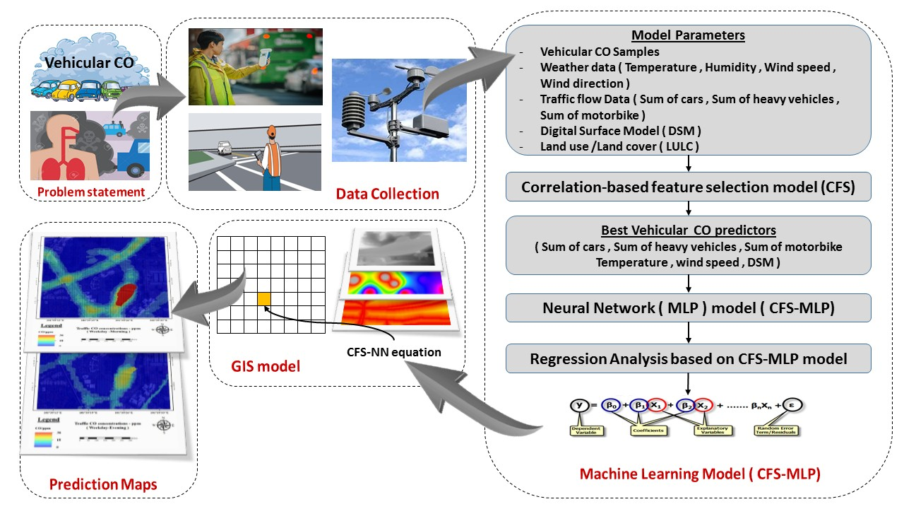
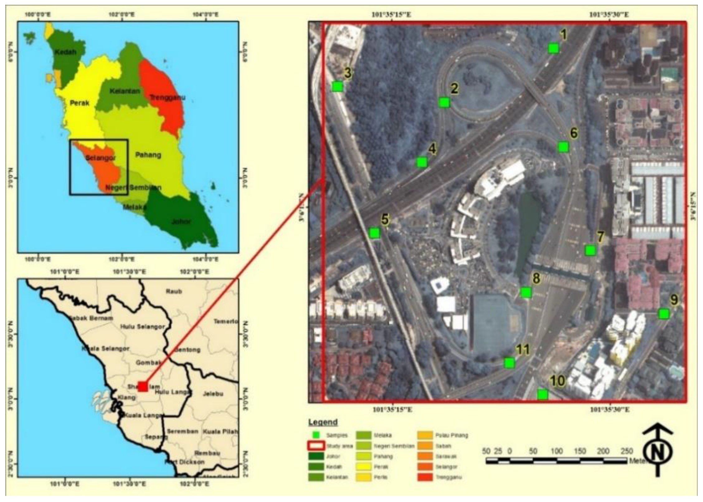
This study was conducted near of Subang jaya toll plaza which links the New Klang Valley Expressway (NKVE) and the federal expressway in Peninsular Malaysia. Subang toll plaza is located within a highly dense populated area in Petaling Jaya, Selangor, Malaysia (Figure 1). The total length of NKVE is 35 km, which connects urban and industrial areas in the capital city of Kuala Lumpur. It is a major highway for citizens who are living in the main cities like Kuala Lumpur, Subang, Shah Alam, Damansara, Sungai Buloh, Klang and Petaling Jaya. The vehicular speed limits are standardized to 110 and 90 km/h on Bukit Raja to Bukit Lanjan stretch and Bukit Lanjan to Jalan Duta stretch, respectively. The study area contains different types of land use such as tollgate area, commercial, industrial and residential areas, making it well suited for vehicular emissions studies.

3.2. Data and Method

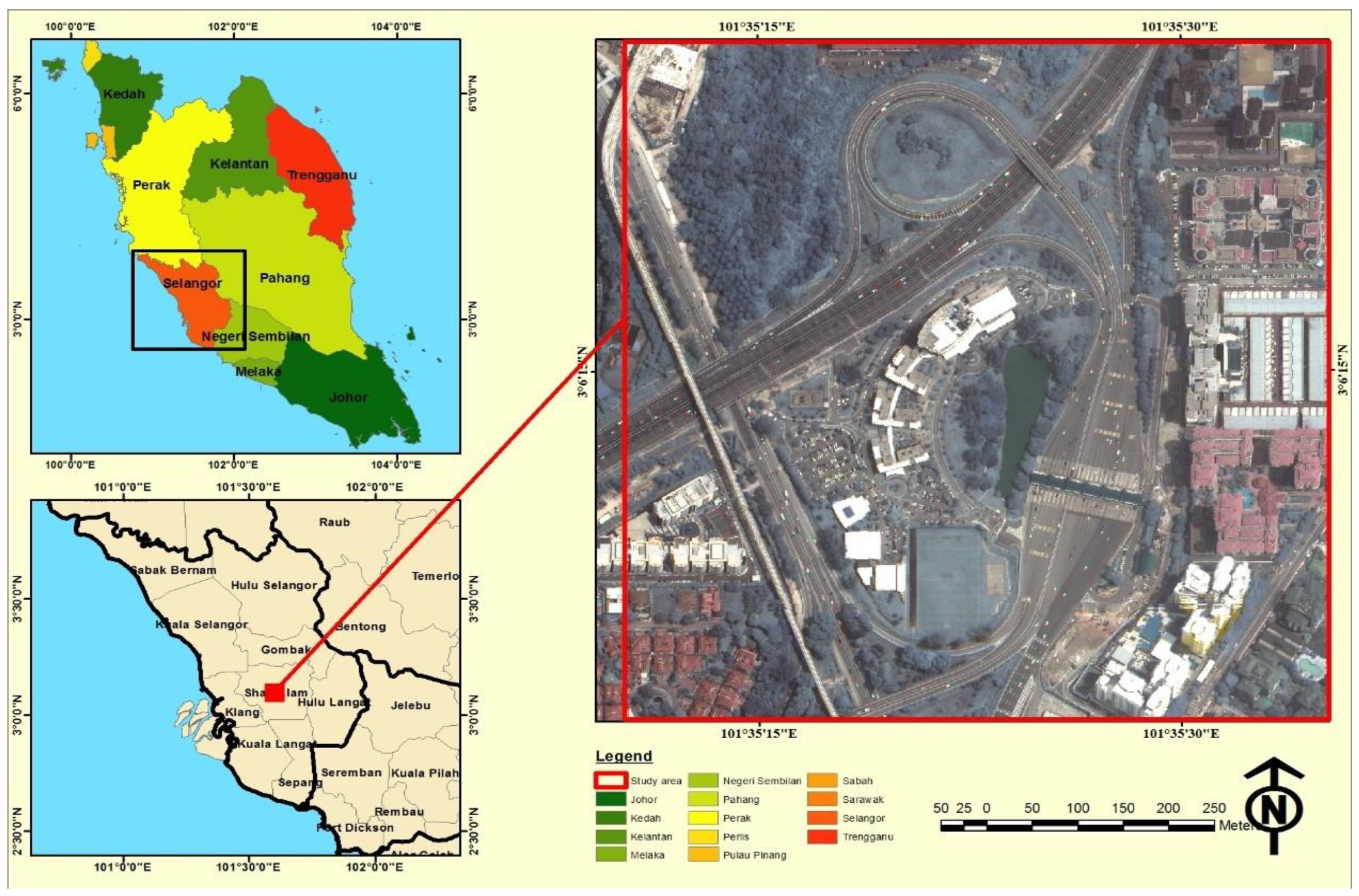
Several data (i.e., vehicular CO samples, meteorology and traffic flow data) were collected from the field during April 2017. Light Detection and Ranging (LiDAR) data were collected in March 2017, and the Worldview3 satellite image was captured in May 2017. Figure 2 shows the overall methodology, which consists of several steps. The hybrid model is designed to predict CO emissions at a specific time and location, for example, prediction maps based on different times of a day. The first step is data collection, which was achieved based on a gas analyzer and data loggers to simultaneously collect CO, temperature, humidity, and traffic information. The LULC map was extracted from the Worldview-3 image with spatial resolution of 0.3 m. The digital surface model (DSM) was derived from the Airborne LiDAR point clouds by using Environment for Visualizing Images (ENVI) software. The second step is the statistical modelling, which was applied by combining two models i.e., the correlation based feature selection (CFS) and Multilayer Perceptron (MLP) by using Weka software. The final step is the spatial modelling based on the regression equations derived from regression analysis and GIS techniques to generate microscale prediction maps for the traffic CO emissions during different times of the day.

3.3. Field Surveying

3.3.1. Sampling Selection

The vehicular CO, traffic condition and meteorology data are important for the development of vehicular CO emissions models [27]. Many studies have described approaches of collecting traffic flow data from the field, and the most important aspect has been determined to be the distribution of air pollutants samples and their suitability [28,29]. The accuracy of the spatial interpolation is highly affected by the sampling design and the variations between traffic CO samples [30]. Moreover, the density of points must be good enough to achieve high accuracy of interpolated data. Conversely, a large number of samples should be avoided to decrease the processing time. Most importantly, the samples density should be adjusted by considering the vehicular CO diffusion characteristics. In this paper, traffic CO data were collected according to a procedure given by [31]. Their method was implemented by creating sampling locations based on a random selection method by using spatial analysis techniques. This approach generates the optimum number of samples compared to the study area [31].

First, three layers (residential, commercial and industrial) from the land-use map were extracted. These layers were converted into points with a spatial constraint to force them inside the land-use polygons. Next, the density of points was estimated using a 150 m search radius and the resolution of the output density raster was set to 25 m. The density rasters were then integrated based on different coefficients (industrial = 1, commercial = 2, and residential = 3). The next step is the rescaling of the final density raster from 0 to 1 depending on linear approach led to the creation of the probability raster which was used to select the samples of the traffic CO. Next, the geospatial balanced points were then created within the study area by using the probability raster. The total number of points were generated based on the length of the road network, the cost of the project and the capability of traffic emissions detection equipment used in the data gathering. As a result, the locations of the traffic CO samples were distributed along the study area. Therefore, extra steps should be implemented to improve the created points in order to select the final sample locations depending on the transportation characteristics. Tessellated grids with a spatial resolution 25 m were generated. Then, these grids were intersected with the created points and the road network layer and the remaining tessellated grids were removed. Subsequently, the final traffic CO samples were selected within the intersected tessellated grids and road network.

3.3.2. Data Collection

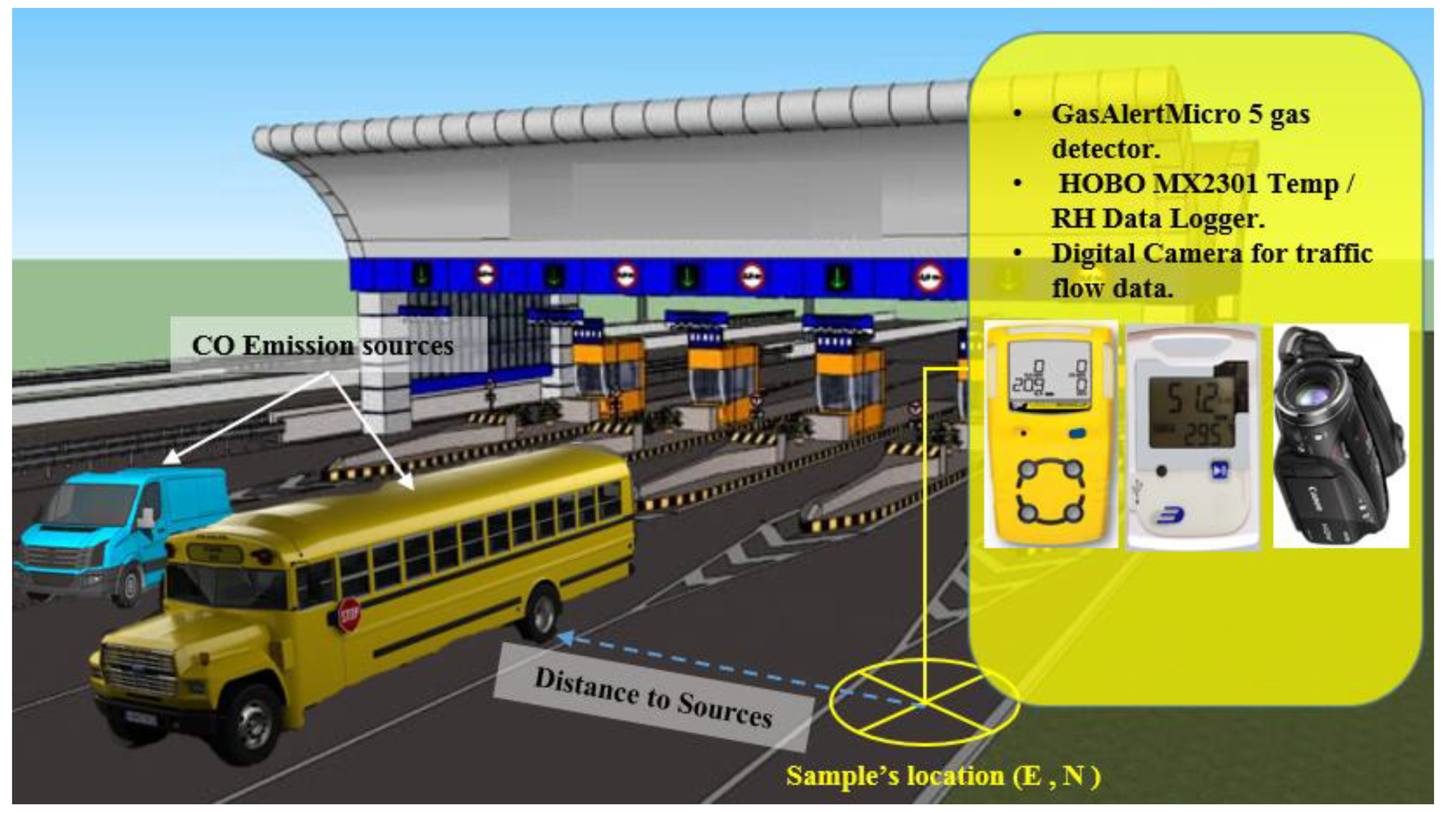
Traffic CO concentrations were collected from the field by using a low cost Gas Analyzer device model Micro-clip5 (1 ppm resolution). The data were collected continuously in 15-min intervals (recording the 15-min minimum, maximum, and average). The traffic flow data and meteorology information were simultaneously collected using a data logger and GPS device (Garmin GPS etrex 10, Olathe, KS, USA; available at University Putra Malaysia). Figure 3 shows the sampling procedure. The traffic CO analyzer was installed in the location of samples by using a Global Navigation System (GPS), at least 2 m from the road edge. The GPS was used to determine the geographic location of samples and to manually verify the locations using land-use maps. The traffic CO was measured four times a day on weekends and weekdays, in the morning (6.30 a.m. to 8.30 a.m.), afternoon (11.30 a.m. to 1.30 p.m.), evening (6.30 p.m. to 8.30 p.m.), and at night (11 p.m. to 12 midnight). In addition, the traffic data were collected by using digital cameras installed in the road’s side in the sample’s location. The traffic flow data were classified into several types (the number of cars, the number of heavy vehicles and the number of motorbikes), where the cars were private cars and taxi cars. On the other hand, the heavy vehicles refer to the following: medium truck, heavy truck, super-heavy/special duty truck and buses, while the motorbikes refer to any type of motorbikes. The meteorological data (temperature, humidity, wind speed and wind direction) were collected for two days, including on weekdays and weekends, to examine various scenarios in the study area for accurate and effective study of traffic CO modelling and mapping (e.g., hazard maps, risk maps, and further analysis). Figure 4 shows the data collection procedure adopted in this study.

3.4. Vehicular CO Prediction Model

3.4.1. Vehicular CO Model Parameters

The presented model aims to predict the daily traffic CO emissions and create prediction maps at different times of a day by using GIS techniques. The traffic CO descriptor (i.e., the dependent parameter) in the current study is the vehicular CO emissions measured every 15 min. The contributing parameters to vehicular CO emission were first selected depending on the previous studies and with consideration of traffic condition, weather characteristics, the surrounding (LULC), topography, and the building heights in the study area. These parameters are the number of vehicles, number of heavy vehicles, the number of motorbikes, temperature, humidity, wind speed, wind direction, LULC and digital surface model (DSM). Many studies have been conducted based on these parameters [32,33,34,35,36]. There are many factors that could affect the vehicular emissions such as engine condition and the fuel type (gasoline, diesel); however, these data cannot be detected through field survey. On the other hand, the data collection did not contain vehicle speed information because the study area is very small and the variation between the vehicles speed is difficult to differentiate. Consequently, the vehicle speed profile is stable during the day. There are many vehicular emissions studies conducted without adopting vehicle speed, such as [25]. The parameters’ statistics are shown in

Table 1. Summary statistics of traffic CO predictors.

Parameter	Average	Minimum	Maximum
Number of vehicles (per 15 min)	1172	126	2762
Number of heavy vehicles (per 15 min)	78	16	325
Number of motorbikes (per 15 min)	112	9	489
Temperature (°C)	29.9	25.6	37.7
Humidity (%)	73.5	54.3	94.5
Wind Speed (mph)	16.87	16	18.20
Wind Direction (angle)	247.1	0	350
DSM (m)	25.7	10.03	129.5

. The NN model was used to find out the degree of contribution of each mentioned parameter for estimating the vehicular CO emission. The NN has the ability to model the complex simulations of non-linear problems such as vehicular CO emission. However, contributing parameters to vehicular CO emission may not be directly used as inputs in the NN model, because of high levels of correlation between the factors resulting in multicollinearity, which can reduce the precision of estimating the vehicular CO emission. Moreover, using a large number of contributing parameters to vehicular CO emission (traffic CO predictors) as input layers of NN can generate over-fitting problems and increase the complexity ratio to run NN model. In the proposed NN model, only relevant and low-correlated parameters were used as inputs. The relevant and significant factors were selected using the CFS model.

Table 2. Summary statistics of traffic CO measurements.

Time	Weekend			Weekday
	Average CO Concentration (per 15 min) (ppm)			Average CO Concentration (per 15 min) (ppm)
	Min	Max	Mean	Min	Max	Mean
Morning	0	8	2.36	0	30.5	8.5
Afternoon	0	14.5	3.5	0	12.8	4.5
Evening	0	9.3	3.92	0	27.3	5.84
Night	0	3.6	1.47	0	5.6	1.9

shows the traffic CO measurements results.

3.4.2. Correlation-Based Feature Selection (CFS) Model

The CFS algorithm is one of the machine learning algorithms which is considered as a filter algorithm that choose the features based on correlation concepts [37]. A major characteristic of the correlation-based function is the ability to choose sub-groups that include features that are unusually correlated to the targeted class but unassociated with each other. On the other hand, this algorithm neglects the features with low correlation with the targeted class, and this algorithm is used to delete the duplicated features because they will be correlated with one of the rest of the features at least. The acknowledgement of a feature will rely on the degree to which it predicts classes in territories of the instance space not currently anticipated by different features.

The CFS’s feature subset assessment function is presented in Equation (1):

$$Ms=k\overline{r_{cf}}/ \sqrt{k+k\left( k-1\right) \overline{r_{ff}}}$$

(1)

where $Ms$ is the heuristic “merit” of a feature subset S containing k features, $\overline{r_{cf}}$ is the mean of the feature-class correlation (f ∈ S), and $\overline{r_{ff}}$ is the average of the feature-feature intercorrelation.

3.4.3. Multilayer Perceptron (MLP) Neural Network

The MLP algorithm is one of the ANN algorithms which results from adding hidden layers to the simple perceptron. In this algorithm, the structure of the NN is generally trained based on backpropagation algorithm and some related variants. Therefore, the models are designed based on the integration of the MLP algorithm and a backpropagation algorithm called backpropagation neural network [38,39,40,41,42,43]. The multilayer perceptron algorithm was developed due to the computational limitations that resulted from single-layered perceptron models. According to the experiments, the multilayer perceptron algorithm has the ability to represent complex simulations and mapping and process high level non-linear problems. Also, the MLP algorithm has the ability to process the nonlinear features, thus allowing the representation of a continuous function of non-linear activation functions such as sigmoid functions [44], which has a clear analogy with the conventional representation of a periodic function such as a Fourier series (i.e., as the sum of simple sine waves). Therefore, the MLP can be considered as a universal functional approximation. Figure 3 shows the architecture of an MLP with several layers of neurons and nonlinear activation functions.

The MLP is considered as a feed-forward system with single or multiple layer of segments among network output and input layers [38,39,40,41,42,43,44,45]. With the assumption of L-layer MPL, the system can signified by $N_{n_0,n_1,\dots , n_L}^L$, where $n_{l }, l=0, 1,\dots ,L$ indicate the number of segments in the input layer $\left(l=0\right)$, the $l$ is number of hidden layers that can range $\left(l=0, 2,\dots ,L-1\right), L$ is the number of layers, and the output layer is $\left(l=L\right)$. $X^{\left(0\right)}={\left[x_0^{\left(0\right)}{u}_1{u}_2\dots u_{n0}\right]}^T$ is the input vector and $X^{\left(l\right)}={\left[x_0^{\left(l\right)}{x}_1^{\left(l\right)}\dots x_{ni}^{\left(l\right)}\right]}^T$ denotes the $l\mathrm{th}$ layer output vector in the interval [0, T]. At this time, $\left\{u_i\right\}$, $j=1,2,\dots n_0$ represents the input attribute pattern while $x_j^{\left(l\right)}$ indicates the output of the jth segments of lth network layer. The threshold input is represented by $x_0^{\left(l\right)}$ with a fixed value at one. The neuron weight of the $j\mathrm{th}$ segment of lth layer from the $i\mathrm{th}$ segment of $\left(l-1\right)$ can be represented by ${\omega }_{ji}^{\left(l\right)}$. The activation function, which is connected with all the segments of the system except the input layer, is the tanh function specified by $\rho \left(S\right)=\tan \mathrm{h}\left(S\right)=\left(\frac{1-e^{-2S}}{1+e^{-2S}}\right)$. The restricted derivative of the $\rho \left(S\right)$ based on $S$ is signified by $\rho \prime \left(S\right)$ that is known as $\rho \prime \left(S\right)$ = $\left(1-{\rho }^2\left(S\right)\right)$. Also, the linear sum of the $j\mathrm{th}$ segment of $l\mathrm{th}$ layer is symbolized by $S_j^{\left(l\right)}$.

In the forward part, at the $k\mathrm{th}$ time direct, the input attribute pattern vector of $X^{\left(0\right)}$ is implemented in the system, while the corresponding preferred output is$\left\{y_j\right\}$, for $j=1,2,\dots ,n_L$. Since no calculation is applied, the input layer of the MLP is known by $x_j^{\left(0\right)}$ = $u_j$ for $j=1,2,\dots ,n_0$. For other layers, $l=1,2,\dots ,L,$ and $j=1,2,\dots ,n_1$, the outputs are computed as:

$$x_j^{\left(0\right)}=\rho (S_j^{\left(l\right)})\mathrm{and} S_j^{\left(l\right)}={\sum }_{i=0}^{ni-1}{\omega }_{ji}^{\left(1\right)}{x}_i^{\left(l-1\right)}.$$

The probable output is identified by $\left\{\widehat{y_{{\displaystyle J}}}\right\}$ and is assumed as $\left\{\widehat{y_{{\displaystyle J}}}\right\}$ $=\left\{x_j^{\left(L\right)}\right\}$ for all $j=1,2,\dots ,n_L$. The mean square error for the system can be formulated as $\frac{e^2}{nL}$ where $e_j=y_j-\widehat{y_{{\displaystyle J}}}$ is the error signal for the $j\mathrm{th}$ output. Furthermore, the instantons squared error can be computed by $e^2={\sum }_{j=1}^{n L}{e}_j^2$.

However, in the learning part, the BP procedure reduces the squared error by varying $\{{\omega }_{ji}^{\left(l\right)}$} according to the gradient search method, recursively. The squared error derivatives connected with the jth segment in layer l are described as Equation (2):

$${\delta }_j^{\left(1\right)}=-\frac{1}{2}\frac{\delta e^2}{\delta S_i^{\left(1\right)}}$$

(2)

Then, these derivatives can be formulated as in Equation (3):

$${\delta }_j^{\left(1\right)}=\{\begin{array}{c}{\rho }^{\prime }\left(S_j^{\left(l\right)}\right).e_j for l=L\hfill \\ {\rho }^{\prime }\left(S_j^{\left(l\right)}\right).{\sum }_{i=1}^{n l+1}{\omega }_i^{\left(l+1\right)}.{\delta }_i^{\left(l+1\right)} for l=L-1,L-2,\dots ,1.\hfill \end{array}$$

(3)

Eventually, the weights of the MLP are reorganized at the kth instant as in Equation (4):

$${\omega }_{ji}^{\left(l\right)}\left(k+1\right)={\omega }_{ji}^{\left(l\right)}\left(k\right)+{\Delta }_{ji}^{\left(l\right)}\left(k\right) and {\Delta }_{ji}^{\left(l\right)}\left(k\right)= \mu {\delta }_i^{\left(l\right)}{x}_i^{\left(l-1\right)}+\gamma {\Delta }_{ji}^{\left(l\right)}\left(k-1\right)$$

(4)

where $\mu$ is the learning rate and $\gamma$ signifies the momentum rate hyper-parameters.

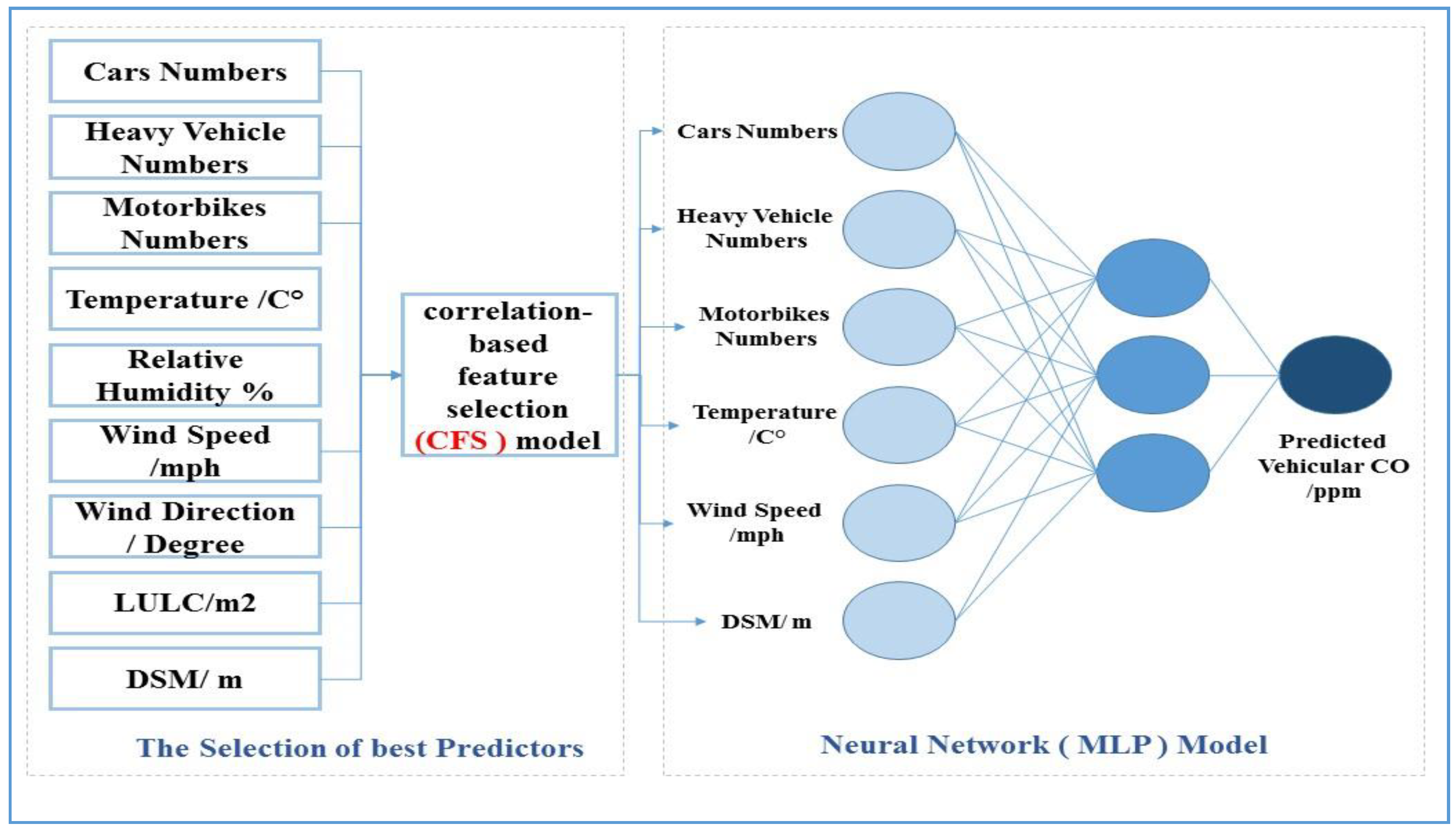
The final proposed network architecture for traffic CO prediction is illustrated in Figure 5. The proposed network is designed based on the results of the best traffic predictors that resulted from the CFS model, optimization and hyper-parameter, which are used to select the best predictors. By using the open source machine learning software (Weka), different MLP structures have been used to select the optimal MLP neural network model for the traffic CO prediction model. The proposed methodology was designed by combining the correlation-based feature selection model and multilayer perceptron.

3.4.4. Optimization Method

The capacity of the prediction in MLP model relies on its hyperparameter and structure. In this paper, several network structure hyperparameter combinations were tested to determine a sub-optimal network model for modeling vehicular CO.

Table 3. Hyper parameters of the proposed model for traffic CO prediction and their search spaces used for fine-tuning.

Parameter	Search Domain
Type of network	MLP, RBF
Number of hidden units	(3–40)
Training Algorithm	BFGS, RBFT
Hidden Activation	Identity, Logistic, Tanh, Exponential, Gaussian
Output Activation	Identity, Logistic, Tanh, Exponential, Gaussian
Learning rate	(0.1, 0.5)
Momentum	(0.1–0.9)

shows the structures and hyperparameters evaluated in the current study and their search space domain. In general, there are two main categories of NN, MLP and radial basis function (RBF). The former uses dot products between inputs and weights and monotonic activation functions such as sigmoid. The MLP uses dot products between inputs and weights and monotonic activation functions such as sigmoid while the RBF uses Euclidean distances between inputs and weights and usually Gaussian activation functions. Both of the networks can be trained with the back-propagation algorithm. In the RBF model, it is not necessary to use multiple hidden layers whereas with MLP, multiple hidden layers are used. In addition, the RBF model is less sensitive to noise than the MLP model. Other parameters of the network are the number of hidden units, training algorithm, error function, activation function, learning rate, and momentum. The number of hidden layers controls the complexity of the designed network. A small number of hidden units may result in low prediction capacity due to insufficient learning whereas a large number of hidden layers can reduce the ability of the model to be generalized and can also create overfitting problems. The training algorithm is the optimization method for calculating the weight for each node in the network. There are many training algorithms for NN based on back-propagation; the Broyden–Fletcher–Goldfarb–Shanno (BFGS) and radial basis function training algorithm (RBFT) are the most recommended back-propagation algorithms used for optimization of NN architecture [46]. During training of the network, an objective function or optimization score function was minimized according to the labeled training dataset. The optimizer usually has a learning rate and gradient momentum parameters. In addition, many activation functions such as identity, logistic, and Gaussian could be used in the hidden layers and the output layers of the neural network.

The total number of instances was 352, which was separated into training 70% (246) and testing 30% (106). This sample size is still small compared to other studies. However, it needs a good approach to handle overfitting problems. One approach is to design a cross-validation evaluation procedure. Other methods are data augmentation or collecting new samples. There are also methods such as transfer learning which requires retrained networks. Overall, training of the neural networks with small datasets requires careful analysis and evaluation before using them in practice. There are also some tricks to improve the performance of neural networks for small datasets. Those include batch normalization, rectified linear unit (relu) activations and regularization methods such as l1 and l2. On the other hand, the hyperparameters of the NN for predicting vehicular CO were chosen based on the implementation of systematic grid-based search that can be applied with the Scikit-Learn algorithm using 100 epochs. Although this method demands high quality of computation, more accurate outputs could result by fine tuning the hyperparameter values. Many models based on various integrations of parameters were generated. Cross validation (10-fold) was applied to validate each model. Therefore, the parameters that resulted in higher accuracy are the best parameters.

3.4.5. GIS Modelling

Collecting traffic CO data, especially on the highways, is dangerous and expensive. Therefore, predicting traffic CO concentrations on highways helps to generate traffic CO data that can be used for further studies. In this research, the measured and predicted traffic CO concentrations are used for GIS modelling based on a grid analysis. GIS modelling and mapping are mainly applied to assess affected people and environments due to inappropriate traffic emissions from traffic activities. The observed traffic CO samples are an important factor in the model, for computing the relationship between the predictive factors and carbon concentrations which were applied in the training data, and for the validation process. After training the NN model with the CO measurements from the field, the NN model produced a regression equation based on weighted values for each predictor factor, in order to calculate the predicted values based on the predictor factors that can be easily applied in a GIS platform; this is the main contribution of the proposed model. This equation has been applied using GIS to produce a spatial prediction of traffic CO concentration in the study area. This step was applied by implementing the final prediction equations on the 5 × 5 m GRID, using ArcGIS tools which are very efficient for spatial representation [23].

4. Results and Discussion

4.1. Contribution of Traffic CO Predictors

As shown in

Table 4. Results of assessing the contribution of traffic CO predictors using the Chi-square method.

Road Traffic CO Predictors	R-Squared	F-Statistic
Number of heavy vehicles	0.7546	32.784
Number of vehicles	0.5322	18.277
Number of motorbikes	0.0472	1.951
DSM (m)	0.0168	1.231
Wind speed (mph)	0.0016	0.124
Temperature (°C)	0.0014	0.1178

, the traffic CO predictors make different contributions to the traffic CO values that resulted from this study. The statistical analysis based on the Chi-square method shows that the parameters that contributed the most are the number of heavy vehicles (F = 32.784) and the number of vehicles (F = 18.277). Conversely, the findings indicated that the other traffic CO predictors (number of motorbikes, DSM, wind speed and temperature) did not make a significant contribution (Table 4).

4.2. Traffic CO Prediction Results

Two MLP models were trained and tested. The first model was trained based on MLP algorithm using nine parameters (those listed in Table 1 plus LULC) to predict the traffic CO concentration. The second model was trained based on the combination with the correlation-based feature selection (CFS-MLP) and six parameters that resulted from the CFS model. These parameters were: number of vehicles, number of heavy vehicles, number of motorbikes, temperature, wind speed, and DSM. The CFS algorithm was implemented to select the highly correlated parameters and best parameters to predict the traffic CO that led to increased accuracy of the prediction process.

Table 5. Results of predictions with MLP model and the proposed model (CFS-MLP) model.

MLP Model		CFS-MLP Model
Best structure	9-4-1	Best structure	6-3-1
Correlation coefficient	0.8657	Correlation coefficient	0.980
Mean absolute error (ppm)	0.991	Mean absolute error (ppm)	0.8925
Root mean squared error (ppm)	1.2862	Root mean squared error (ppm)	1.2736
Relative absolute error %	30.94%	Relative absolute error %	21.99%
Root relative squared error %	23.48%	Root relative squared error %	19.40%
Total number of instances	247	Total number of instances	247

shows the proposed model’s results when the input parameters were filtered and reduced from nine parameters to six based on the CFS algorithm which finds features that have higher correlation with the class but are uncorrelated with each other. Therefore, the highest correlated parameters were used for the prediction analysis, which resulted in improving the prediction accuracy. The relative absolute error decreased from 30.94% to 21.99% and the root relative square error also decreased from 23.48% to 19.40%. On the other hand, the correlation coefficient increased from 0.866 ppm to 0.98 ppm. The mean absolute error (MAE) was reduced from 0.99 ppm to 0.89 ppm. The root mean square error (RMSE) also decreased from 1.29 ppm to 1.27 ppm. The prediction results showed that the prediction improvement occurred after the implementation of the CFS algorithm which is able to reduce the high dimensionality, remove the low correlated data and improve the learning accuracy.

4.3. Traffic CO Prediction at Different Times of Day

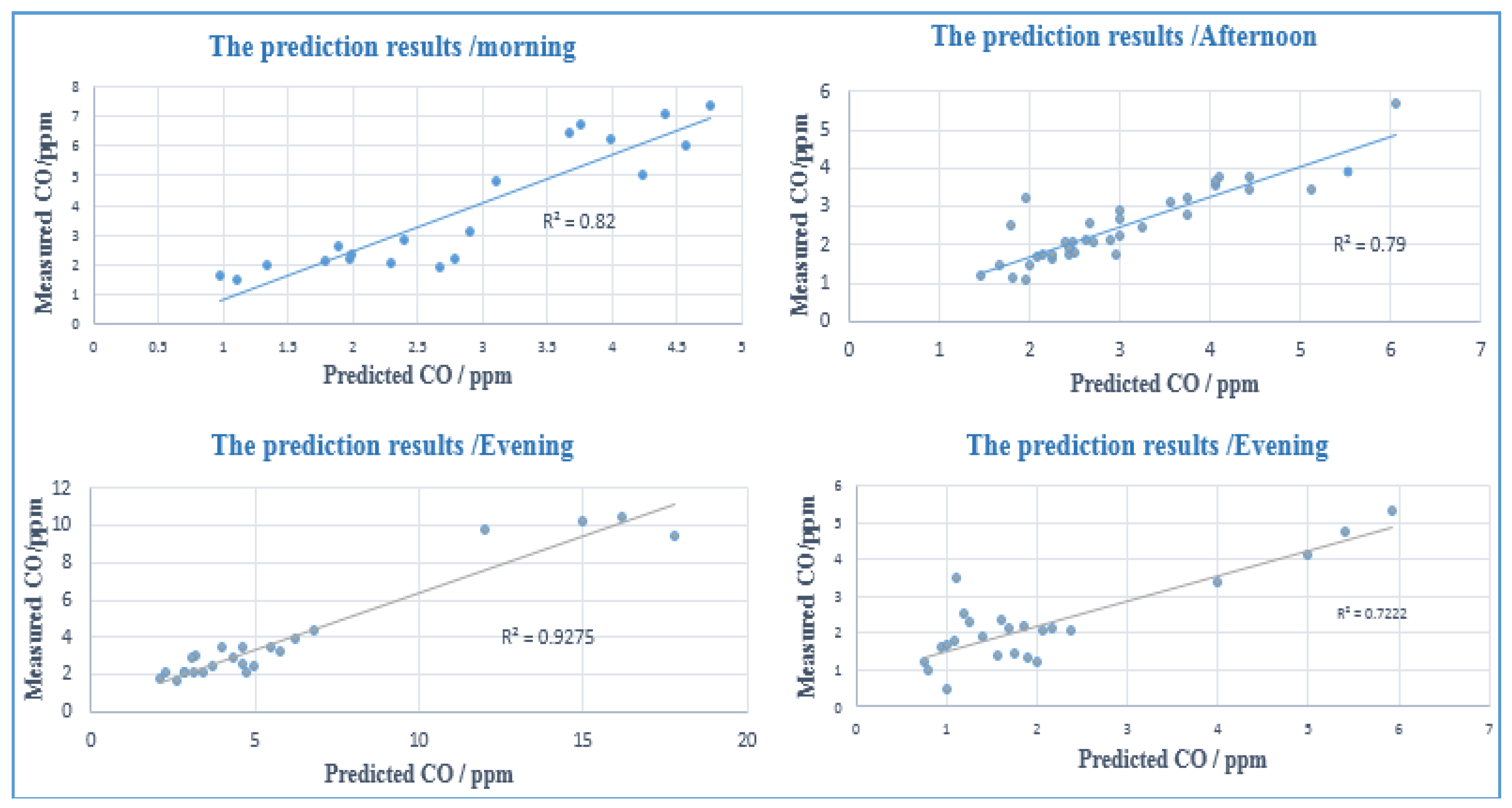
Regression equations were created, based on the results from the CFS-MLP model; the coefficients of vehicular emissions predictors are calculated to formulate regression models to easily predict vehicular emission in the study area using a set of predictors that can be gathered from the field and existing databases in order to facilitate connection with the GIS-based model by applying parameter coefficients in the spatial model. The decision makers can notice the effect of causative parameters on vehicular emissions occurrence, which was assessed by the corresponding coefficient that appears in the regression function [47]. Regression equations were simulated at different times during the day (morning, afternoon, evening and night) to predict traffic CO at these times. The highest RMSE was 2.9817 ppm during evening observations, while the lowest RMSE was 0.387 ppm at night.

Table 6. Regression models for traffic CO prediction based on the CFS-MLP model.

Traffic CO Predictors	Estimated Coefficient
	Morning	Afternoon	Evening	Night
Number of vehicles	−0.0016	0.0142	0.0108	0.0147
Number of heavy vehicles	0.0622	0.01	0.0319	−0.0216
Number of motorbikes	0.0135	−0.0378	−0.0376	−0.0093
Temperature °C	−0.4501	0.5512	0.4888	−0.0333
Wind speed mph	0.0752	−0.194	−0.4084	0.0135
DSM m	−0.2085	0.213	0.0812	0.1116
Intercept	16.8559	−22.2525	−15.8113	−2.1367
RMSE	2.914 ppm	2.0347 ppm	2.9817 ppm	0.387 ppm

shows the results of the regression analysis at different times.

4.4. GIS Modelling Results

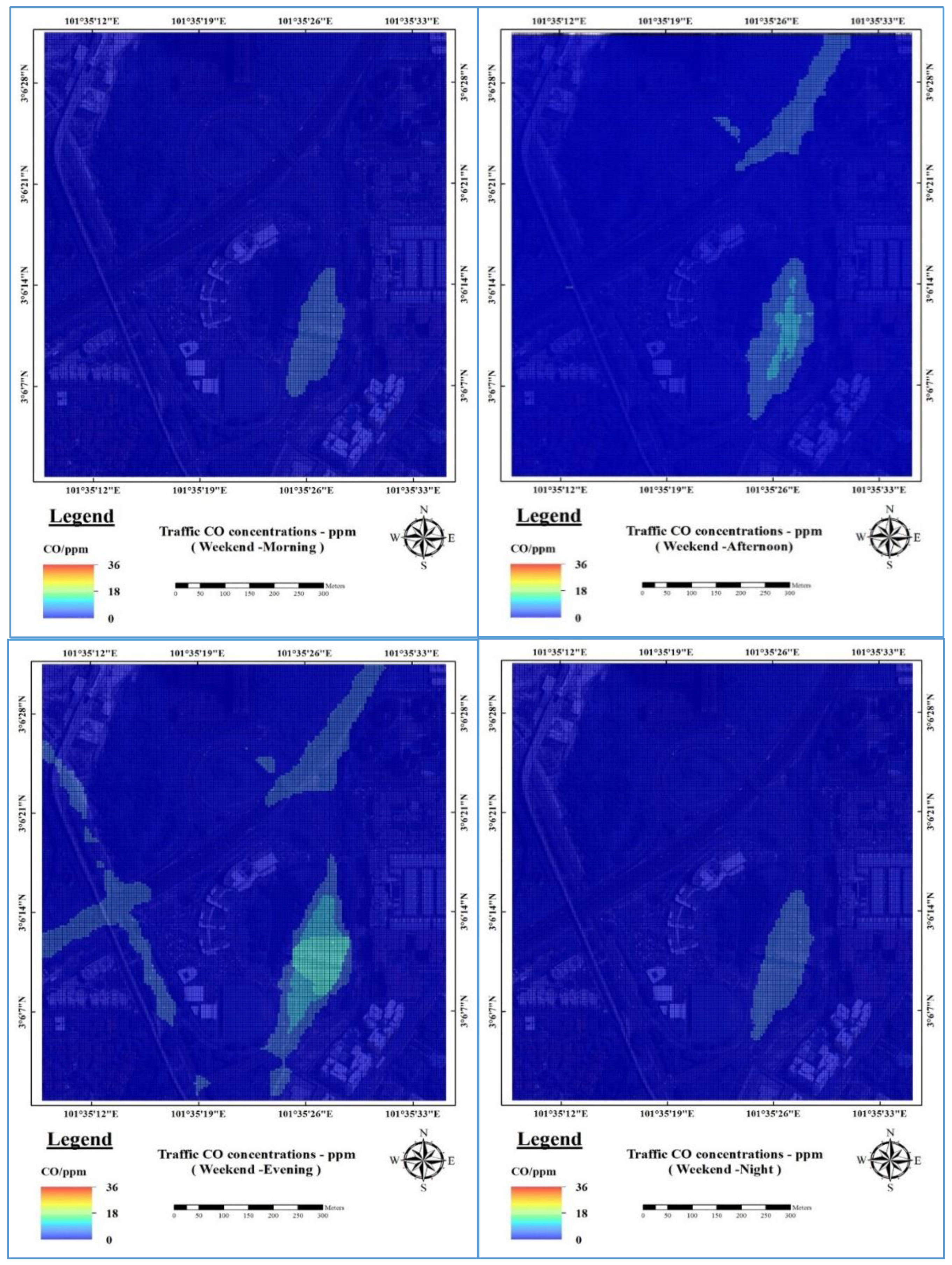
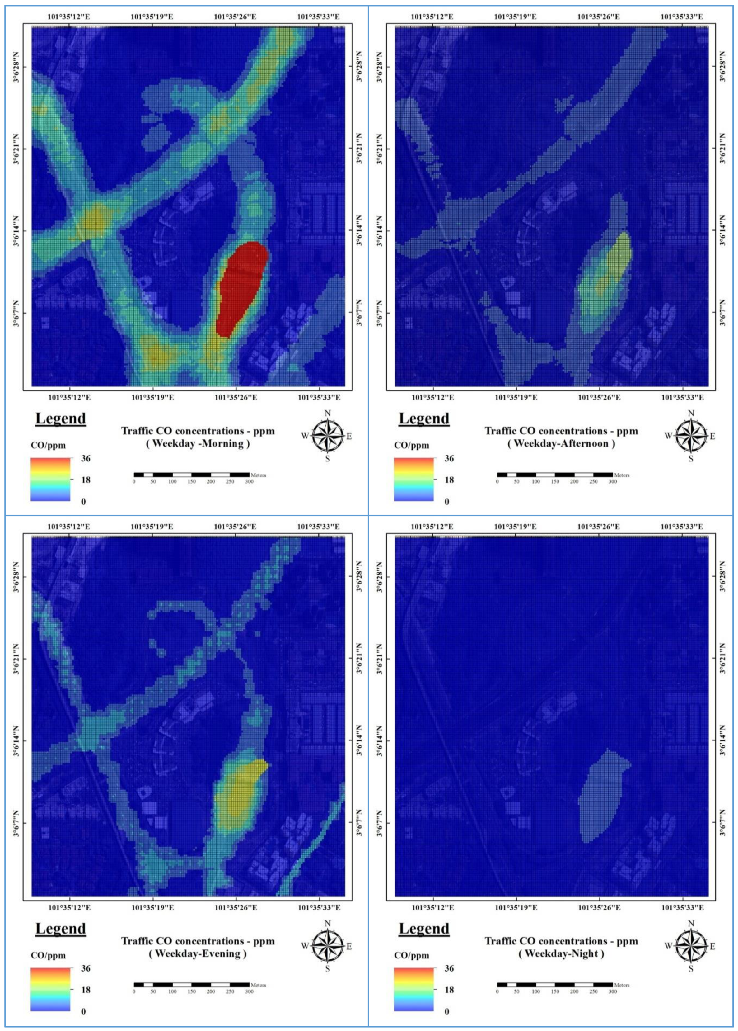
A GIS model was applied to generate prediction maps at different times a day (Figure 6 and Figure 7). The resultant spatial prediction maps showed that the concentrations of traffic CO increased more on weekdays than on weekends. These maps also showed that there was significant variation between traffic CO concentrations according to the time of day, with the traffic CO ranging from a high of 35.23 ppm per 15 min during the weekday morning to a low of 4.76 ppm per 15 min during the weekend night. The prediction maps showed that the highest values of traffic CO are located near the toll areas compared to other areas such as residential green areas, because of the traffic congestion at toll gates. The lowest values of traffic CO are concentrated near residential areas which reached zero values.

4.5. Comparison with Other Models

The developed model was compared with other popular models such as the support vector machine for regression (SVR) and the linear regression (LR) models. These models generated two statistical equations based on model parameters. Testing data were used for model validation; these equations are shown below:

$$\begin{array}{cc}\hfill \mathrm{Traffic}\mathrm{CO}=& 0.0022\times \mathrm{Number}\mathrm{of}\mathrm{vehicles}+0.0403\times \mathrm{Number}\mathrm{of}\mathrm{heavy}\mathrm{vehicles}\hfill \\ & \hspace{1em}-0.0187\times \mathrm{Number}\mathrm{of}\mathrm{Motorbikes}+0.1957\times \mathrm{Temperature}\hfill \\ & \hspace{1em}-0.0984\times \mathrm{Wind}\mathrm{speed}-0.0102\times \mathrm{DSM}-4.4382\hfill \end{array}$$

(4)

For the LR model:

$$\mathrm{Traffic}\mathrm{CO}= 0.05\times \mathrm{Number}\mathrm{of}\mathrm{heavy}\mathrm{vehicles}+0.21$$

(5)

4.6. Validation of Traffic CO Prediction Maps

The traffic CO spatial prediction maps were verified using the test sites of traffic CO samples, and the verification method was then performed by comparing the traffic CO test data and the traffic CO spatial prediction maps. The lowest accuracy of the validation was at night time (72.48%) and the highest accuracy was during the evening (92.75%).

Table 7. The comparison between CFS-MLP, SVR and LR models.

CFS-MLP Model		SVR Model		LR Model
Correlation coefficient	0.980	Correlation coefficient	0.8668	Correlation coefficient	0.851
Mean absolute error (ppm)	0.896	Mean absolute error (ppm)	1.640	Mean absolute error (ppm)	1.851
Root mean squared error (ppm)	1.286	Root mean squared error (ppm)	2.752	Root mean squared error (ppm)	2.849
Relative absolute error (%)	21.99	Relative absolute error (%)	51.646	Relative absolute error (%)	55.048
Root relative squared error (%)	19.40	Root relative squared error (%)	49.784	Root relative squared error (%)	48.292
Total number of instances	247	Total number of instances	247	Total number of instances	247

shows the comparison between CFS-MLP, SVR and LR model. The comparative analysis was conducted by using the training data and the proposed model, support vector regression model, linear regression, land use regression model and dispersion model i.e., CALINE4 model based on many criteria not only Root mean square RMSE, but we also compared the proposed model with other baseline models based on mean absolute error (MAE), relative absolute error, root relative squared error and correlation coefficient. Results showed that the proposed model is superior to the compared models. The correlation coefficient based on our proposed model was 0.980, which is higher than the SVR (0.8668) and LR (0.851). The MAE of the proposed model was 0.896 ppm which is lower than SVR (1.640 ppm) and LR (1.851 ppm). On the other hand, the RMSE results indicated that the proposed model has the lowest RMSE (1.286 ppm) compared to SVR (2.752 ppm) and LR models (2.849 ppm). The RAE ratio for the proposed model was calculated to be 21.99%, which was lower than the RAE ratio of SVR (51.646%) and LR (55.048%). The root relative squared error indicated that the proposed model has the lowest value (19.40%) among the other models (49.784% and 48.292%).

Table 7 shows the comparison between CFS-MLP, SVR and LR model. The comparative analysis was conducted by using the training data and the proposed models, i.e., SVR, LR, land use regression model and dispersion model, i.e., CALINE4 model based on many criteria, not only RMSE. We also compared the proposed model with other baseline models based on mean absolute error (MAE), relative absolute error, root relative squared error and correlation coefficient. Results showed that the proposed model is superior to the other models. The CO emission prediction rate can be justified as highly accurate, where the accuracy is more than 90%; 90% to 80% is a good forecast; 80% to 50% is a reasonable forecast; and more than 50% is an inaccurate forecast [48,49,50].

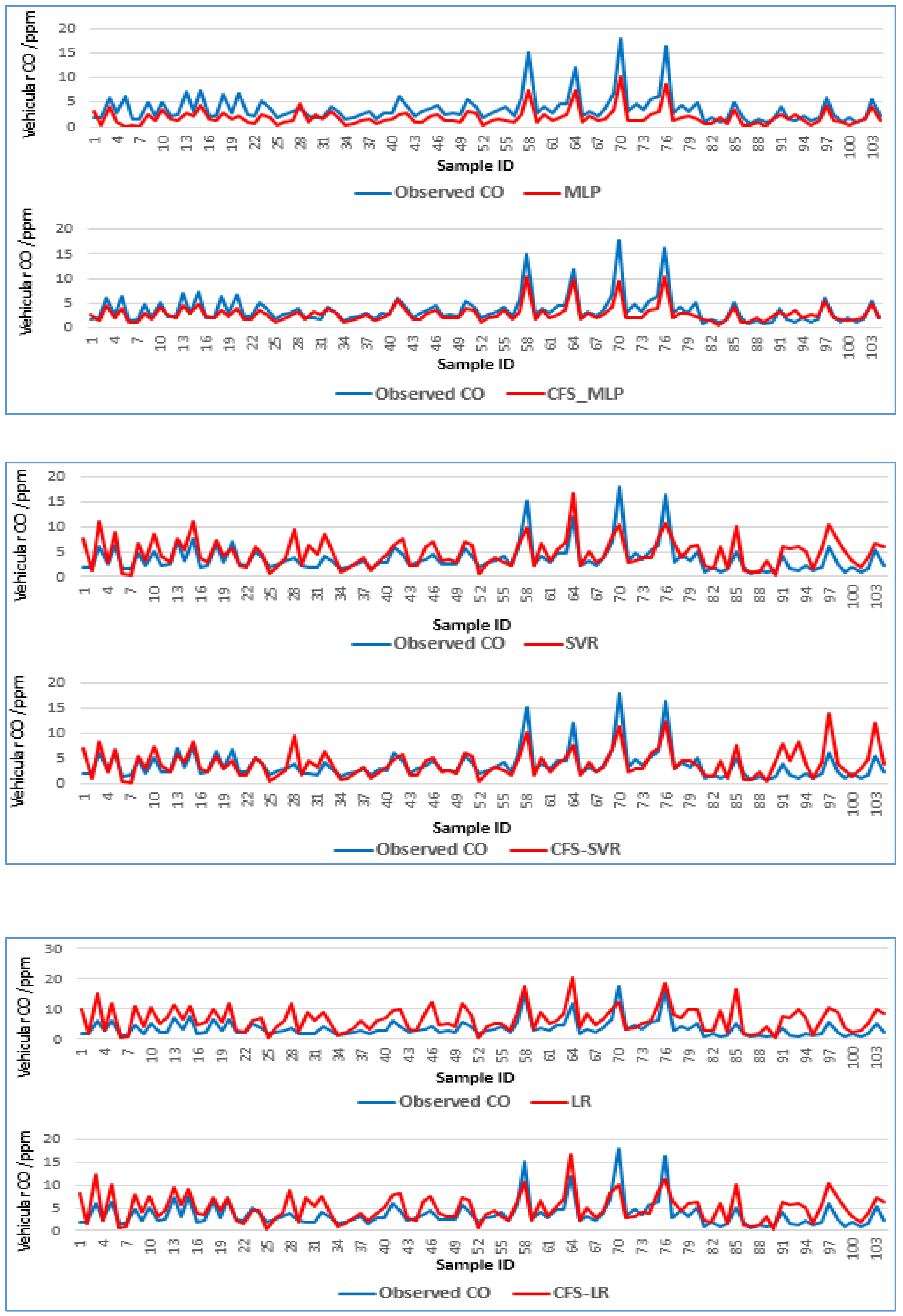
The correlation coefficient based on our proposed model was 0.980, which is higher than the SVR (0.8668) and LR (0.851). The MAE of the proposed model was 0.896 ppm which is lower than SVR (1.640 ppm) and LR (1.851 ppm). On the other hand, the RMSE results indicated that the proposed model has the lowest RMSE (1.286 ppm) compared to SVR (2.752 ppm) and LR models (2.849 ppm). The RAE ratio for the proposed model was calculated to be 21.99%, which was lower than the RAE ratio of SVR (51.646%) and LR (55.048%). The root relative squared error indicated that the proposed model has the lowest value (19.40%) among the other models (49.784% and 48.292%).

Table 8. The comparison between CFS-MLP, CFS-SVR and CFS-LR models.

CFS-MLP Model		CFS-SVR Model		CFS-LR Model
Correlation coefficient	0.980	Correlation coefficient	0.7578	Correlation coefficient	0.82
Mean absolute error (ppm)	0.896	Mean absolute error (ppm)	1.972	Mean absolute error (ppm)	1.9713
Root mean squared error (ppm)	1.286	Root mean squared error (ppm)	3.7109	Root mean squared error (ppm)	3.1057
Relative absolute error (%)	21.99	Relative absolute error (%)	64.3605	Relative absolute error (%)	64.333
Root relative squared error (%)	19.40	Root relative squared error (%)	67.2464	Root relative squared error (%)	56.2795
Total number of instances	247	Total number of instances	247	Total number of instances	247

shows the results of the prediction models when combining the correlation-based feature selection; the correlation coefficients of the CFS-SVR and CFS-LR are 0. 0.7578 and 0.82, respectively. These values indicated that there is decrease in the correlation coefficient. The MAE increased for the CFS-SVR and CFS-LR and reached 1.972 ppm and 1.9713 ppm, respectively. The EMSE also increased to 3.7109 ppm and 3.1057 ppm. Figure 8 illustrates the variations of the traffic CO concentrations in the testing data.

The first model that we compared with one of the baseline models is the CALINE4 model. The CALINE4 model is a dispersion model, which depends on a plume dispersion model used to predict the vehicular CO on roadways [48]. The CALINE4 model simulates the data based on a Gaussian diffusion algorithm and characterizes the pollutants dispersion on roads. We defined the proposed road network, weather data, traffic flow information, and receptor locations, and the prediction of traffic CO emissions was obtained. The MAE and RMSE values were 2.376 ppm and 4.2254 ppm, respectively, whereas and the correlation coefficient value was 0.6504. The prediction results appeared worse than our proposed model. This may due to the fact that the Gaussian diffusion, which was assumed in CL4, is not very realistic.

We also compared our work with the Land Use Regression (LUR) Model. This model is generally applied to predict air pollutants depending on the land use, traffic flow information, meteorology data and combined them based on a linear regression algorithm. The LUR model showed the following values: MAE 2.21 ppm, RMSE 4.50 ppm and a correlation coefficient of 0.5989 (Figure 9).

The final LUR equation used is given below:

Predicted CO = 0.0018 × Car + 0.0423 × HV − 0.0219 × Motorbike + 0.2211 ×
Temp/C + 0.0312 × Relative Humidity − 0.1315 × Wind speed + 0.0018 × Wind
Angle Degree − 0.0232 ∗ DSM + 0.0006 × Builtup area + 0.0064 × Highway −
8.6627.

There are many models developed based on GIS and machine learning, for example [26] designed a model based on the integration of the ANN algorithm and the linear-chain conditional random field algorithm to produce real-time and fine-grained air pollution prediction maps.

The air quality data were obtained from fixed air quality stations, the traffic data were collected from vehicle trajectory, and the meteorology data were collected from monitoring stations. Other data used were land use, road geometry and social information. Their results presented the prediction maps with low resolution, cell size (1 × 1) km² in local scale. The limitation of this model can be summarized in some points. The data collection from the standard fixed air quality monitoring stations may not be able to measure the air quality that people are exposed on the ground level due to the limitation of monitoring location and height. On the other hand, the data obtained from the fixed stations are not suitable for high-resolution prediction maps such as microscale maps. Moreover, this study did not contain information about the terrain and buildings.

The proposed model in this research is different from the aforementioned study based on some points. We developed a GIS-based NN and data were obtained from a field survey. Moreover, the land use and DSM were extracted from a very high resolution LiDAR data clouds. The proposed methodology is designed to predict the vehicular CO and produce high-resolution maps at a microscale level (5 × 5) m² whereas the aforementioned paper estimated air pollutants based on a low-resolution grid (1 × 1) km².

Regarding the meteorology parameters shown in Table 4, it is evident that the correlation between wind speed and vehicular emissions is 0.0016, which is considered weak in the short-term prediction and in a small area compared to other factors. In addition, the temperature has the lowest correlation with vehicular emissions 0.0014; therefore, the variation in the vehicular emissions (i.e., CO) may not be significantly affected by the weather condition in the prediction in small areas. On the other hand, the DSM, which was used to extract the terrain and building’s altitude in the study area, has a good correlation with vehicular emissions (more than meteorology parameters). Therefore, the geographic factors are important in prediction studies. This study adopted high-resolution elevation data in order to extract results that are more accurate. In urban areas, building altitude is an important parameter because it can resist vehicular emissions and prevent the distribution of pollutants in urban areas.

5. Conclusions

Traffic emissions (e.g., traffic CO) are considered the major source of air pollution in congested urban areas, including road corridors in toll plaza areas. Traffic emission prediction models are utilized to evaluate the impacts of traffic CO emissions on the population and environment and some models are used to illustrate the spatial prediction of these emissions. In this paper, a hybrid prediction model was proposed by combining three models (CFS, MLP and GIS) to predict the traffic CO emissions and create micro-scale prediction maps in a small area at different times during the day. The final findings have shown that the proposed model scored an accuracy of 80.6% and the correlation coefficient of 0.980, RMSE of 1.2736 ppm and mean absolute error of 0.8925 ppm. We used CFS to identify and remove highly correlated parameters so that redundancy was reduced to choose the optimum parameters used in the prediction model through MLP. The simulation results showed that nine predictors were reduced to six, which contributed to an increase in the prediction accuracy.

The data were collected from the field and remote sensing data (i.e., LiDAR and very high-resolution WorldView-3 satellite image), and modelling was performed in a GIS environment.

In this study, we produced microscale maps for vehicular emissions. The simulated traffic CO emissions ranged from 35 ppm inside the toll plaza area to 0 ppm for areas that were located far away from the toll area. As per the microscale-prediction maps, high spatial variation in the traffic CO emissions was identified. The highest value of CO concentrations is found in traffic jam areas. Conversely, the lowest values of traffic CO emissions are distributed far from traffic activities. The highest concentrations of traffic CO were located inside the toll plaza because of the traffic jam that occurs daily in the toll areas these results give a clear indication about the relationship between the traffic activities and the traffic CO emissions. The traffic CO emissions may have a significant impact on the health of toll plaza workers, drivers and the passengers. Therefore, such a prediction model can aid decision makers to implement plans to mitigate the traffic emissions that can protect people who are working, passing through or living near toll plaza areas; this will be the main advantage of the proposed forecasting system.

Traffic CO emission prediction models and GIS modeling are both efficient tools for transportation planning and traffic emission assessment. The prediction maps produced by the proposed model can be used as an effective tool in the decision-making process to identify optimum solutions which can be used to mitigate traffic jams in toll plaza areas as well as on highways and road networks. As traffic emission pollution assessment by decision makers is very complicated and usually expensive because of the high level of requirements for expert knowledge and the developed support systems, the presented traffic CO assessment model is not expensive and can easily implemented. Moreover, the traffic CO pollution concentrations vary based on the traffic condition and the number of vehicles, which requires a periodic monitoring of traffic emissions by government agencies or relevant departments. The best parameter selection analysis could be used to reduce the data collection requirements, which can lead to reduced time required, resources utilized and processing time needed. GIS modeling is a useful tool for non-expert users to implement the traffic CO impact assessments in various applications. Finally, these models can be improved by using more advanced algorithms such as deep learning algorithms and a large number of samples that can be used to increase the accuracy of the prediction process.

References

- Bastien, L.A.; McDonald, B.C.; Brown, N.J.; Harley, R.A. High-resolution mapping of sources contributing to urban air pollution using adjoint sensitivity analysis: Benzene and diesel black carbon. Environ. Sci. Technol. 2015, 49, 7276–7284. [Google Scholar] [CrossRef] [PubMed]
- Fameli, K.M.; Assimakopoulos, V.D. Development of a road transport emission inventory for Greece and the Greater Athens Area: Effects of important parameters. Sci. Total Environ. 2015, 505, 770–786. [Google Scholar] [CrossRef] [Green Version]
- Borge, R.; Narros, A.; Artinano, B.; Yagüe, C.; Gomez-Moreno, F.J.; de la Paz, D.; Quaassdorff, C. Assessment of microscale spatio-temporal variation of air pollution at an urban hotspot in Madrid (Spain) through an extensive field campaign. Atmos. Environ. 2016, 140, 432–445. [Google Scholar] [CrossRef]
- Oftedal, B.; Krog, N.H.; Pyko, A.; Eriksson, C.; Graff-Iversen, S.; Haugen, M.; Aasvang, G.M. Road traffic noise and markers of obesity–a population-based study. Environ. Res. 2015, 138, 144–153. [Google Scholar] [CrossRef]
- Ancona, C.; Badaloni, C.; Mattei, F.; Cesaroni, G.; Stafoggia, M.; Forastiere, F. Health Impact Assessment of Air Pollution, Noise, and Lack of Green in Rome. J. Transp. Health 2017, 5, S42–S43. [Google Scholar] [CrossRef]
- Garshick, E.; Laden, F.; Hart, J.E.; Caron, A. Residence near a major road and respiratory symptoms in US veterans. Epidemiology 2003, 14, 728. [Google Scholar] [CrossRef] [PubMed]
- Delfino, R.J.; Tjoa, T.; Gillen, D.L.; Staimer, N.; Polidori, A.; Arhami, M.; Longhurst, J. Traffic-related air pollution and blood pressure in elderly subjects with coronary artery disease. Epidemiology 2010, 21, 396–404. [Google Scholar] [CrossRef]
- Crouse, D.L.; Goldberg, M.S.; Ross, N.A.; Chen, H.; Labrèche, F. Postmenopausal breast cancer is associated with exposure to traffic-related air pollution in Montreal, Canada: A case–control study. Environ. Health Perspect. 2010, 118, 1578. [Google Scholar] [CrossRef]
- Domene, E.; Lopez, R.; Fauro, B.; Rojas-Rueda, D.; Conill, C.; Alsina, G.; Marull, J. Modelling Impacts of Mobility on Urban Air Quality and Health: Scenario Analysis for the Barcelona Metropolitan Area (Metropolitan Mobility Plan). J. Transp. Health 2017, 5, S60–S61. [Google Scholar] [CrossRef]
- Singh, D.; Kumar, A.; Kumar, K.; Singh, B.; Mina, U.; Singh, B.B.; Jain, V.K. Statistical modeling of O3, NOx, CO, PM2. 5, VOCs and noise levels in commercial complex and associated health risk assessment in an academic institution. Sci. Total Environ. 2016, 572, 586–594. [Google Scholar] [CrossRef] [PubMed]
- Behera, S.N.; Sharma, M.; Mishra, P.K.; Nayak, P.; Damez-Fontaine, B.; Tahon, R. Passive measurement of NO2 and application of GIS to generate spatially-distributed air monitoring network in urban environment. Urban Clim. 2015, 14, 396–413. [Google Scholar] [CrossRef]
- Johnson, M.; Isakov, V.; Touma, J.S.; Mukerjee, S.; Özkaynak, H. Evaluation of land-use regression models used to predict air quality concentrations in an urban area. Atmos. Environ. 2010, 44, 3660–3668. [Google Scholar] [CrossRef]
- Kanaroglou, P.S.; Adams, M.D.; De Luca, P.F.; Corr, D.; Sohel, N. Estimation of sulfur dioxide air pollution concentrations with a spatial autoregressive model. Atmos. Environ. 2013, 79, 421–427. [Google Scholar] [CrossRef]
- Vandaele, N.; Van Woensel, T.; Verbruggen, A. A queueing based traffic flow model. Transp. Res. Part D Transp. Environ. 2000, 5, 121–135. [Google Scholar] [CrossRef]
- Tomić, J.; Bogojević, N.; Pljakić, M.; Šumarac-Pavlović, D. Assessment of traffic noise levels in urban areas using different soft computing techniques. J. Acoust. Soc. Am. 2016, 140, EL340–EL345. [Google Scholar] [CrossRef]
- Hamad, K.; Khalil, M.A.; Shanableh, A. Modeling roadway traffic noise in a hot climate using artificial neural networks. Transp. Res. Part D. Transp. Environ. 2017, 53, 161–177. [Google Scholar] [CrossRef]
- Di Mascio, P.; Di Vito, M.; Loprencipe, G.; Ragnoli, A. Procedure to determine the geometry of road alignment using GPS data. Procedia-Soc. Behav. Sci. 2012, 53, 1202–1215. [Google Scholar] [CrossRef]
- Righini, G.; Cappelletti, A.; Ciucci, A.; Cremona, G.; Piersanti, A.; Vitali, L.; Ciancarella, L. GIS based assessment of the spatial representativeness of air quality monitoring stations using pollutant emissions data. Atmos. Environ. 2014, 97, 121–129. [Google Scholar] [CrossRef]
- Hülsmann, F.; Gerike, R.; Ketzel, M. Modelling traffic and air pollution in an integrated approach–the case of Munich. Urban Clim. 2014, 10, 732–744. [Google Scholar] [CrossRef]
- Kim, Y.; Guldmann, J.M. Land-use regression panel models of NO2 concentrations in Seoul, Korea. Atmos. Environ. 2015, 107, 364–373. [Google Scholar] [CrossRef]
- Zarandi, M.F.; Faraji, M.R.; Karbasian, M. Interval type-2 fuzzy expert system for prediction of carbon monoxide concentration in mega-cities. Appl. Soft Comput. 2012, 12, 291–301. [Google Scholar] [CrossRef]
- Kwok, L.K.; Lam, Y.F.; Tam, C.Y. Developing a statistical based approach for predicting local air quality in complex terrain area. Atmos. Pollut. Res. 2017, 8, 114–126. [Google Scholar] [CrossRef]
- Quaassdorff, C.; Borge, R.; Pérez, J.; Lumbreras, J.; de la Paz, D.; de Andrés, J.M. Microscale traffic simulation and emission estimation in a heavily trafficked roundabout in Madrid (Spain). Sci. Total Environ. 2016, 566, 416–427. [Google Scholar] [CrossRef]
- Shakerkhatibi, M.; Mohammadi, N.; Zoroufchi Benis, K.; Behrooz Sarand, A.; Fatehifar, E.; Asl Hashemi, A. Using ANN and EPR models to predict carbon monoxide concentrations in urban area of Tabriz. Environ. Health Eng. Manag. J. 2015, 2, 117–122. [Google Scholar]
- Cai, M.; Yin, Y.; Xie, M. Prediction of hourly air pollutant concentrations near urban arterials using artificial neural network approach. Transp. Res. Part D Transp. Environ. 2009, 14, 32–41. [Google Scholar] [CrossRef]
- Zheng, Y.; Liu, F.; Hsieh, H.P. U-Air: When urban air quality inference meets big data. In Proceedings of the 19th ACM SIGKDD International Conference on Knowledge Discovery and Data Mining, Chicago, IL, USA, 11–14 August 2013; pp. 1436–1444. [Google Scholar]
- Namdeo, A.; Mitchell, G.; Dixon, R. TEMMS: An integrated package for modelling and mapping urban traffic emissions and air quality. Environ. Model Softw. 2002, 17, 177–188. [Google Scholar] [CrossRef]
- Kho, F.W.L.; Law, P.L.; Ibrahim, S.H.; Sentian, J. Carbon monoxide levels along roadway. Int. J. Environ. Sci. Technol. 2007, 4, 27–34. [Google Scholar] [CrossRef] [Green Version]
- Ranjbar, H.R.; Gharagozlou, A.R.; Nejad, A.R.V. 3D analysis and investigation of traffic noise impact from Hemmat highway located in Tehran on buildings and surrounding areas. J. Geogr. Inf. Syst. 2012, 4, 322. [Google Scholar] [CrossRef]
- Li, F.; Liao, S.S.; Cai, M. A new probability statistical model for traffic noise prediction on free flow roads and control flow roads. Transp. Res. Part D Transp. Environ. 2016, 49, 313–322. [Google Scholar] [CrossRef]
- Ragettli, M.S.; Goudreau, S.; Plante, C.; Fournier, M.; Hatzopoulou, M.; Perron, S.; Smargiassi, A. Statistical modeling of the spatial variability of environmental noise levels in Montreal, Canada, using noise measurements and land use characteristics. J. Expos. Sci. Environ. Epidemiol. 2016, 26, 597. [Google Scholar] [CrossRef]
- Kirchstetter, T.W.; Singer, B.C.; Harley, R.A.; Kendall, G.R.; Chan, W. Impact of oxygenated gasoline use on California light-duty vehicle emissions. Environ. Sci. Technol. 1996, 30, 661–670. [Google Scholar] [CrossRef]
- Goyal, P. Present scenario of air quality in Delhi: A case study of CNG implementation. Atmos. Environ. 2003, 37, 5423–5431. [Google Scholar] [CrossRef]
- Chen, K.S.; Wang, W.C.; Chen, H.M.; Lin, C.F.; Hsu, H.C.; Kao, J.H.; Hu, M.T. Motorcycle emissions and fuel consumption in urban and rural driving conditions. Sci. Total Environ. 2003, 312, 113–122. [Google Scholar] [CrossRef]
- Henderson, S.B.; Beckerman, B.; Jerrett, M.; Brauer, M. Application of land use regression to estimate long-term concentrations of traffic-related nitrogen oxides and fine particulate matter. Environ. Sci. Technol. 2007, 41, 2422–2428. [Google Scholar] [CrossRef]
- Shi, Y.; Lau, K.K.L.; Ng, E. Developing street-level PM2.5 and PM10 land use regression models in high-density Hong Kong with urban morphological factors. Environ. Sci. Technol. 2016, 50, 8178–8187. [Google Scholar] [CrossRef]
- Hall, M.A. Correlation-Based Feature Selection for Machine Learning. Ph.D. Thesis, The University of Waikato, Hamilton, New Zealand, 1999. [Google Scholar]
- Boznar, M.; Lesjak, M.; Mlakar, P. A neural network-based method for short-term predictions of ambient SO2 concentrations in highly polluted industrial areas of complex terrain. Atmos. Environ. Part B Urban Atmos. 1993, 27, 221–230. [Google Scholar] [CrossRef]
- Chaloulakou, A.; Saisana, M.; Spyrellis, N. Comparative assessment of neural networks and regression models for forecasting summertime ozone in Athens. Sci. Total Environ. 2003, 313, 1–13. [Google Scholar] [CrossRef]
- De Cos Juez, F.J.; Nieto, P.G.; Torres, J.M.; Castro, J.T. Analysis of lead times of metallic components in the aerospace industry through a supported vector machine model. Math. Comput. Model. 2010, 52, 1177–1184. [Google Scholar] [CrossRef]
- Gardner, M.W.; Dorling, S.R. Neural network modelling and prediction of hourly NOx and NO2 concentrations in urban air in London. Atmos. Environ. 1999, 33, 709–719. [Google Scholar] [CrossRef]
- Hooyberghs, J.; Mensink, C.; Dumont, G.; Fierens, F.; Brasseur, O. A neural network forecast for daily average PM10 concentrations in Belgium. Atmos. Environ. 2005, 39, 3279–3289. [Google Scholar] [CrossRef]
- Kukkonen, J.; Partanen, L.; Karppinen, A.; Ruuskanen, J.; Junninen, H.; Kolehmainen, M.; Cawley, G. Extensive evaluation of neural network models for the prediction of NO2 and PM10 concentrations, compared with a deterministic modelling system and measurements in central Helsinki. Atmos. Environ. 2003, 37, 4539–4550. [Google Scholar] [CrossRef]
- Nieto, P.G.; Lasheras, F.S.; García-Gonzalo, E.; de Cos Juez, F.J. PM 10 concentration forecasting in the metropolitan area of Oviedo (Northern Spain) using models based on SVM, MLP, VARMA and ARIMA: A case study. Sci. Total Environ. 2018, 621, 753–761. [Google Scholar] [CrossRef]
- Friedman, J.; Hastie, T.; Tibshirani, R. The Elements of Statistical Learning; Springer Series in Statistics: New York, NY, USA, 2001; Volume 1. [Google Scholar]
- Rojek, I. Technological process planning by the use of neural networks. AI EDAM 2017, 31, 1–5. [Google Scholar] [CrossRef]
- Mousavi, S.Z.; Kavian, A.; Soleimani, K.; Mousavi, S.R.; Shirzadi, A. GIS-based spatial prediction of landslide susceptibility using logistic regression model. Geomat. Nat. Hazards Risk 2011, 2, 33–50. [Google Scholar] [CrossRef] [Green Version]
- Sharma, N.; Gulia, S.; Dhyani, R.; Singh, A. Performance evaluation of CALINE 4 dispersion model for an urban highway corridor in Delhi. J. Sci. Ind. Res. 2013, 72, 521–530. [Google Scholar]
- Pao, Y.-H.; Phillips, S.M.; Sobajic, D.J. Neural-net computing and the intelligent control of systems. Int. J. Control 1992, 56, 263–289. [Google Scholar] [CrossRef]
- Pao, H.-T.; Fu, H.-C.; Tseng, C.-L. Forecasting of CO2 emissions, energy consumption and economic growth in China using an improved grey model. Energy 2012, 40, 400–409. [Google Scholar]
Figure 1.
Location map of the study area.
Figure 2.
The overall methodological flow chart employed in this study.
Figure 3.
The sampling locations.
Figure 4.
Location of traffic CO and meteorological parameter measurement on a highway section.
Figure 5.
The architecture of the proposed neural network for traffic CO prediction (6-3-1).
Figure 6.
Prediction maps during the weekend at different times (morning, afternoon, evening and night).
Figure 7.
Prediction maps during weekdays at different times (morning, afternoon, evening and night).
Figure 8.
Accuracy assessment of the predicted maps (morning, afternoon, evening and night).
Figure 9.
Comparison between the proposed and other models.