Design and Simulation of a Capacity Management Model Using a Digital Twin Approach Based on the Viable System Model: Case Study of an Automotive Plant

Abstract

Matching supply capacity and customer demand is challenging for companies. Practitioners often fail due to a lack of information or delays in the decision-making process. Moreover, researchers fail to holistically consider demand patterns and their dynamics over time. Thus, the aim of this study is to propose a holistic approach for manufacturing organizations to change or manage their capacity. The viable system model was applied in this study. The focus of the research is the clustering of manufacturing and assembly companies. The goal of the developed capacity management model is to be able to react to all potential demand scenarios by making decisions regarding labor and correct investments and in the right moment based on the needed information. To ensure this, demand data series are analyzed enabling autonomous decision-making. In conclusion, the proposed approach enables companies to have internal mechanisms to increase their adaptability and reactivity to customer demands. In order to prove the conceptual model, a simulation of an automotive plant case study was performed, comparing it to classical approaches.

1. Introduction

In a fast-changing environment with increasing demand volatility, shorter product life cycles, new technologies, and new trade regulations, balancing supply capacity and market demand is a challenge for organizations all over the world. In this context, the capability of an organization to change as an adaptability characteristic is key in order to secure its viability. As a consequence, global managers are under increasing pressure to make decisions more quickly.

While new technologies open new possibilities, many managers, even in well-established companies, do not have a system or virtual digital twin to enable them to foresee the expected outcomes of decisions that are to be made. Neither complete information nor all the implications of a decision are appropriately considered in most organizations. Because of this, many managers usually decide to start a process of collecting information to conduct an analysis as the basis for decision-making regarding capacity. This process involves different areas. Therefore, the decision is delayed until it has to be made, implying the loss of profit generation, as customers are not buying products due to a lack of capacity or long delivery times as a result.

For all of these reasons, this paper attempts to provide an answer to those managers and their daily planning challenges by providing a conceptual model and a simulation of a case study. As a consequence, the practical relevance of this paper is a digital interface for decision-making support including technical, management, and economic key performance indicators. This interface provides a platform that can be used to avoid unnecessary investments, increase sales for all types of manufacturing companies, reduce operating costs, and support higher service levels. Moreover, the theoretical relevance of the paper is a novel approach that combines already consolidated scientific methods into a new concept for demand and capacity planning that is oriented to end-customer demand.

The purpose of this paper is to develop a generic conceptual model for capacity planning in which decisions can be sped up in order to adapt them as quickly as possible to demands considering a level of risk for investments and changes in the production system. That is why economic parameters are considered to balance potential profit generation with investments or costs incurred. In this regard, the concept development presents different levels: network planning, location-related planning, and line planning within a location. With these three levels it can be taken into account whether it is a greenfield or brownfield scenario and whether it involves a new product launch.

The main hypothesis is that a manufacturing company capable of adapting its capacity to demand using the structure of the viable system model (VSM) will be able to react faster and, therefore, applying this model will have a positive impact on the achievement of short-, medium-, and long-term goals of production companies. The VSM approach increases the adaptability of a company to face future potential scenarios, because the company will be able to make strategic decisions that will later influence the tactical and operative levels.

Based on the conceptual model, a case study for an original equipment manufacturer (OEM) was chosen. It is a brownfield scenario in which there is a new product launch in a production line with two models using the same platform. By proving different scenarios and decisions to be made, the conceptual model is proven in order to check the hypothesis previously set.

2. Fundamental Definitions and State of Research

The literature review shows that there are about 30 basic methods that help to predict future sales, many of them with subtypes [1]. The purpose of demand planning is to improve decisions that affect demand accuracy [2]. Its main task is to calculate future demand, and it comprises the selection of a specific forecasting method and its parameters. The typical demand patterns are stationary, seasonal, trend, and sporadic [3].

Independent of the demand type, the bullwhip effect is a challenge in every supply chain due to the lack of transparency between stages. As a result, it is frequently difficult to forecast the final customer demand based on orders along the supply chain [4], and this causes an extreme fluctuation of stock at the beginning of the supply chain, creating many backorders alternating with large excess inventory [5].

To combat the bullwhip effect, there should be information sharing of consumer demand across the supply chain in order to allow each party to plan efficiently according to true demand information [6].

Collaborative forecasting and planning are the basis for capacity management through the supply chain. Capacity utilization, like stock levels and work in progress, is one of the degrees of freedom of planning and control in supply chains. An assessment of the necessary capacitive resources is a task in every planning period. Supply flexibility in medium- and short-term planning often requires long-term arrangements [5] such as investments in production capacity.

To decide on investments properly, it is necessary to focus on the system limitations. A constraint can be the management of an organization, capacities along the supply chain, or market demand. In this context, the theory of constraints (TOC) provides a framework to deal with capacity management issues with five steps: identify the constraint, exploit the constraint, subordinate the rest of the system to the constraint before increasing capacity, then add new capacities and start other times by finding the capacity constraint [7].

There are four procedures, from short to long term, to adapt supply capacity to demand requirements.

• Extra hours or reduction of hours: This approach is closely related to the “additional shift” process; it allows great flexibility and is used with the advantage of existing employees.
• Additional shifts: This alternative allows dealing with short-term demand fluctuations. Extra costs and training depend on the demand fluctuation and staff availability.
• External production: This is used to react to demand peaks; it results mainly in higher unit prices and has the risk of knowledge transfer.
• Investments: This option requires good predictions of capacity needs, because, as capacity increases, fixed costs also increase.

There are multiple customer implications of a lack of capacity, from delays to market share losses. The consequences of bottlenecks are as follows [8]:

• Limited availability;
• Long delivery times with decreasing reliability;
• Constantly changing priorities and quantities;
• Errors and cancellations;
• High personal commitment of the employees involved in order processing;
• Additional expenditure due to extensive internal clarifications or the search for external alternative suppliers;
• Additional costs through partial and express deliveries, special shifts, and temporary employees;
• Individual decisions instead of overall optimum.

If this condition remains over time, customer satisfaction decreases, and companies lose market share and sales potential. Investments are not immediate and, therefore, do not alleviate the bottleneck in the short term and have the risk of being oriented too much to short-term needs and an overcapacity situation developing in the long term [8].

As a consequence, key indicators for capacity-related decision-making should be defined taking into account that the final goal of each business activity is to increase the value of the company [9]. The main indicators for an investment are return on investment (ROI), the payback period, and the net present value (NVP). Moreover, it is also important to consider the concept of opportunity cost of not making a decision on an investment, for instance, cars not sold due to a bottleneck in the paint shop.

In conclusion, after having calculated those indicators with an assumed demand pattern, other risks should be considered, such as demand volatility, new market entrance, price sensitivity, promotions, etc.

3. Methodology

Cooperation between research partners and the chosen methodological approach was set as a combination of an in-depth literature review, conceptual development, and simulation techniques in a specific case study. The study refers to manufacturing companies with a production network, plant, or group of machines with a certain capacity to serve a specific market.

The method used to reach the goal of matching market demand started from analyzing the structure to develop the conceptual model. For this purpose, the viable system model (VSM) was selected. The VSM is a cybernetic model that was developed by Beer throughout his life [10]. The viable system model is a reference model that can be applied to describe, diagnose, and design management models in organizations [11]. Beer deduced the VSM from cybernetics, and from the central nervous system of the human being, in order to deal with complex systems [12]. Through the analysis of the central nervous system, the minimum requirements that a system must meet to ensure that it is viable were derived [13]. In this way, each sub-system has one of the nervous system’s functions. The nervous system is composed of units that execute actions, such as the spine, muscles, and organs (System 1), the spinal cord (System 2), the brain stem (System 3), the diencephalon (System 4), and the cerebral cortex (System 5) [11]. Analogous to the planning levels of a company, the structure of the VSM can be divided into three levels. Therefore, Systems 1–3 (including System 3*) are assigned to the operational level. System 4, in turn, represents the level of strategic planning and stabilizes the entire system thanks to its interaction with the environment. System 5, finally, represents the level of normative planning [11].

Moreover, in order to determine which policies should be used to control the behavior over time and how these policies should be designed and implemented in order to have a robust response against change [14], system dynamics was chosen. Vensim, a software package enabling system dynamics modeling, was selected for this project. Vensim is a software program that allows for the simulation of highly complex and dynamic systems that involve a lot of integrated decision-making. Vensim (Vensim is a registered trademark of Ventana Systems Inc.) provides a high degree of rigor for writing model equations. It adds features for tracing feedback loops. Vensim also provides very powerful tools for the optimization of multi-parametric simulation results, which allows the analysis to validate results and the model’s structure, as well as to determine the most convenient policy options by parameterizing these policies.

The innovative approach relies on a combination of the following, in order to generate a decision-making support concept and model in Vensim for balancing supply and demand over time for a specific production system including economic influences:

• The viable system model as a framework for developing the conceptual model;
• System dynamics for designing and controlling the production system’s behavior;
• Statistical process control for demand pattern monitoring;
• Forecasting methods for calculating a demand forecast per period.

Once the methods were set, an in-depth literature review of demand planning, capacity planning, and adaptability, along with key indicators for capacity-related decision-making, was performed. As a result, the basis for the conceptual model development was built. It is an integrated model created for all kinds of manufacturing organizations. Later, the generic conceptual model was extrapolated and proven for the case study of an OEM plant. A simulation was programmed in Vensim using assumptions, and validation with extreme values was performed. Finally, different scenarios and decisions were simulated in order to test the hypothesis previously defined.

4. Design and Simulation of the Conceptual Model for Capacity Planning of an OEM Plant

4.1. Design of a Generic Conceptual Model Development Applying the VSM

The VSM environment is represented by customer demand, technological change, quality standards, price, and capacity of competitors. System 5, the normative level of capacity management, determines the goals of ROI and payback standards. System 4 considers the environment and internal set-up and situation in order to make decisions to match supply capacity with customer demand. Decisions are made depending on the reactivity, i.e., the risks to be taken when making a decision, such as making an investment or adding an additional shift. System 3 determines the overall internal planning using a certain forecasting method as well as methods for demand and capacity planning. Moreover, economic parameters are consolidated here. System 2 represents the coordination of the production lines or shops within the production plant to achieve production goals. Finally, System 1 contains the entities or machine groups within a production line or a workshop. In order to support capacity management activities, these groups are viewed as machine groups that can produce the same products. In order to develop the conceptual model, the following activities were performed:

• Development of an economic target system depending on capacity utilization of a production network, plant, line, or group of machines;
• Capacity management tasks according to planning horizon levels;
• Definitions of recursion levels and operative units;
• Association of tasks to recursion levels and operative units;
• Identification of needed information flows between operative units and recursion levels.

The conceptualization of capacity management based on the viable system model, and the tasks related to the five systems of the viable system model are shown in Figure 1.

In the different recursion levels, casual loop diagrams were constructed in order to identify interrelationships among factors. Moreover, the main characteristics of the conceptual model that applies the viable system model are described below and compared with the classical approach, named the nonviable system model.

Demand planning: There are control limits based on statistical process control principles, such as the time series in quality control charts and hypothesis tests that are used to change a demand forecasting method to another method.

The classical approach uses one method (simple moving average) to forecast customer demand, while the VSM simulation model can change between two forecasting models (simple linear regression and cumulative moving average) depending on the pattern of the demand. Moreover, the VSM simulation model is able to detect outliers, forecast sporadic trends, extend the moving average, and detect seasonal demands.

• The focus of demand forecasting is not to bring about a difference between the models in terms of the accuracy of the used forecast methods, but to be able to respond to the changes in customers’ demands by detecting the pattern changes as soon as possible. Due to this premise, the model includes factors that allow for controlling the values that trigger the forecasting changes. Therefore, it is a fight between “detecting only the changes that are real changes” (but perhaps not before they have a negative impact on production and sales parameters) or “detecting more changes than the real ones but knowing that, if there is a change, it is going to be anticipated” (but knowing that, if a change is not a real one, the system will have more forecast failures at first).
• This viable system model deals with uncertainty in demand by calculating forecast values for each product separately. Then, the forecast for groups of customers is done by aggregation of customers′ forecasts.

Forecasting models: There are three methods in requirements planning: demand-driven or deterministic, stochastic, and heuristic. Each forecasting method is adequate for a certain demand pattern, as shown in Figure 2 [15]. As mentioned above, one important characteristic of the viable system model is its ability to adapt its demand forecasting. As a consequence, it is able to detect demand pattern changes after it starts forecasting with another method or with the same method but with different parameters. The approach tries to respond as quickly as possible to demand transformations. In so doing, the model can detect fake changes, which would be worthwhile due to its fast reaction capability.

The VSM model recognizes the following patterns, and it forecasts them with the forecasting methods listed:

• Trend: with regression analysis.
• Trend plus sporadic: with regression analysis plus an average sporadic quantity per day.
• Sporadic: the sum of outliers is divided by their frequency to obtain the average demand per day.
• Steady: with the cumulative moving average method.
• Steady plus sporadic: with the cumulative moving average method plus an average sporadic quantity per day.
• Seasonal: with the cumulative moving average method (however, this is not the appropriate forecast method in terms of accuracy for this kind of demand pattern).

The system is able to detect the following changes by analyzing historical demand data:

• From steady to steady with a lower/higher mean;
• From steady to steady with a lower/higher standard deviation;
• From steady to steady plus a positive/negative sporadic pattern;
• From steady to an increasing/decreasing trend;
• From trend to trend plus a positive/negative sporadic pattern;
• From trend to steady;
• From trend to seasonal;
• From a sporadic pattern to another sporadic pattern.

All of these changes are controlled by the variable called “demand reactivity”. This variable affects all of the control limits for the changes described above. When the value of this variable is higher, then the VSM simulation model detects more changes in demand with less accuracy but reacts before real changes occur in the demand pattern. Each of these changes has a lower and an upper control limit. These limits are fixed using a statistical approach that assumes the forecasting parameters have a normal distribution.

It can be seen as a hypothesis test. We use the first type of detection (from steady to steady with a lower/higher mean) as an illustrative example. If the mean of the last 10 days (the sample) for the customer is lower/higher than the mean that is used for forecasting (the population) minus/plus one standard deviation, then a new steady pattern is created with a lower/higher mean, because, with a high percentage, the last 10 values are not a sample of the population (the last demand pattern).

• H_o = the mean is the same as before: the null hypothesis is accepted when mean of the last 10 values is within the control limits that are the mean plus/minus one standard deviation.
• H₁ = the mean is higher/lower: one of the alternative hypotheses is accepted if the mean of the last 10 values is not within the control limits.

As was explained in the first detection case, the other changes are tracked using the same methodology.

Capacity planning: This has an influence on the decision on the number of shifts, the number of employees, and new investments, each of which has a certain delay until its implementation. The conceptual model compares, for each period of time, the gap between demand and available capacity. Based on it and on the demand planning, which is based on a forecasting method and a statistical analysis, the following measures are considered in the conceptual model:

• Adjust the number of employees in order to produce more in the same number of shifts.
• Adjust the number of shifts, as well as working hours, on weekends or holidays.
• Increase external production capacities for peak or constant production requirements.
• Increase the production capacity with new investments.
• Calculate the daily production loss according to bottlenecks and extrapolate it for longer periods based on the available demand forecast.
• Increase maintenance planning and coordination, as well as the number of tools, in order to reduce breakdowns and increase plant availability.

Economic parameters: Within the conceptual model, three decisions are considered.

• New investments for increasing production capacity. For this decision, the model requires a payback of less than two years. The return on investment is forecast to determine the increase in capacity that is pursued by the investment.
• Operational costs related to extra hours or extra shifts of operational employees. Based on the gap between production capacity and demand, operational costs are optimized by adjusting the number of employees, working days, and shifts.
• Customer demand loss based on the value of the customer order lead time. Customers buy from a company or not depending on the lead time. Therefore, the model assesses the customer requirements and evaluates the losses in sales due to a long delivery process. Based on this loss, a decision on whether to improve capacity and internal processes can be made.

Decision-making: Decision trees are used as a function of the level, i.e., network, plant, line, machine group. For decision-making, a simulation inside the simulation is conducted in order to make a forecast of the decision, taking into account the risk of the decision with a qualitative approach of price sensitivity and new market entrance. To predict the behavior, quality standards for time series are used to analyze the probability that a demand pattern will continue over time (assumption: a demand pattern is only influenced by customer needs, not market influence, normative standards, price, promotions, disasters, etc.).

4.2. Simulation of a Specific Model for the Case Study of an Automotive Plant

The following assumptions were made:

• Time restrictions: Firstly, the modeler must define a time horizon and units of time. It is easy to carry out this step by asking to what extent the simulation should be considered. In the case of the study, it was decided to simulate four working years to evaluate influences in the medium and long term. The simulation was performed with 1000 time periods, each representing one producing day counting in total for four years of production.
• Production capacity has a maximum of 600 units per day in three shifts at the beginning of the simulation. During the simulation, two investment options were considered: an increase of 100 units per day or an increase of 200 units per day. Both models assessed the same requirements for initiating one or the other investment. The difference between the viable system model and the nonviable system model was the lead time of the decision-making process.

  ○

  Viable system model: the decision-making process takes 10 days.

  ○

  Nonviable system model: the decision-making process takes 100 days.

• Demand characteristics and forecast: The model makes different forecasts using two methods, i.e., moving average and linear regression:
  • Moving average: the simple moving average (SMA) is the non-weighted mean of the previous n data [16]. In the nonviable system model, it is calculated as the average for the last 10 days (n = 10). As the VSM is able to detect demand changes over time, all demand values were taken into account for the forecast until a new demand pattern was registered. Therefore, the formula of the cumulative moving average was applied.
  • Linear regression: The regression analysis method is usually applicable to a steady course of a time series or a stable trend [16]. In the model, it is only used for trend demand patterns, when using only one leading indicator and the time since the trend demand pattern was detected. As a result, a simple linear regression can be defined as follows:

    F _j (t) = demand forecast for customer j at time t = α × t_trend + β,

    where α is the slope, t_trend is the time since the trend demand pattern was detected, and β is the value at the time when the trend demand pattern was detected.
• The existing car model is in a mature stage with stable demand and provides 1000 euros/car of margin. The new model is in the process of being launched and provides 2000 euros/car. These values were used to calculate profits. If there is loss in volume, it is assumed that the new model will have the loss in volume due to unknown future demand.
• The simulation model considers sales loss starting from a customer order lead time greater than 60 days.
• A product is a finished product after it leaves the production facility.
• The warehouses have no stock limitation.
• There is no transport limitation (or limitation to the number of trucks) between the different stages.
• A steady supply of materials for the production process is provided.
• The available stock, as well as the number of products, is known at every moment of the transport process.
• Order information along the supply chain is available.
• Data on historical demand are available for both models one day after the demand.
• Operational adjustments allow for changing the shift model with a one-third increase in the capacity per extra shift with a maximum of three shifts. Moreover, a higher number of employees in an existing shift provide a flexibility of 10% to existing production capacities.
• Production is 50% make-to-stock and 50% make-to-order.
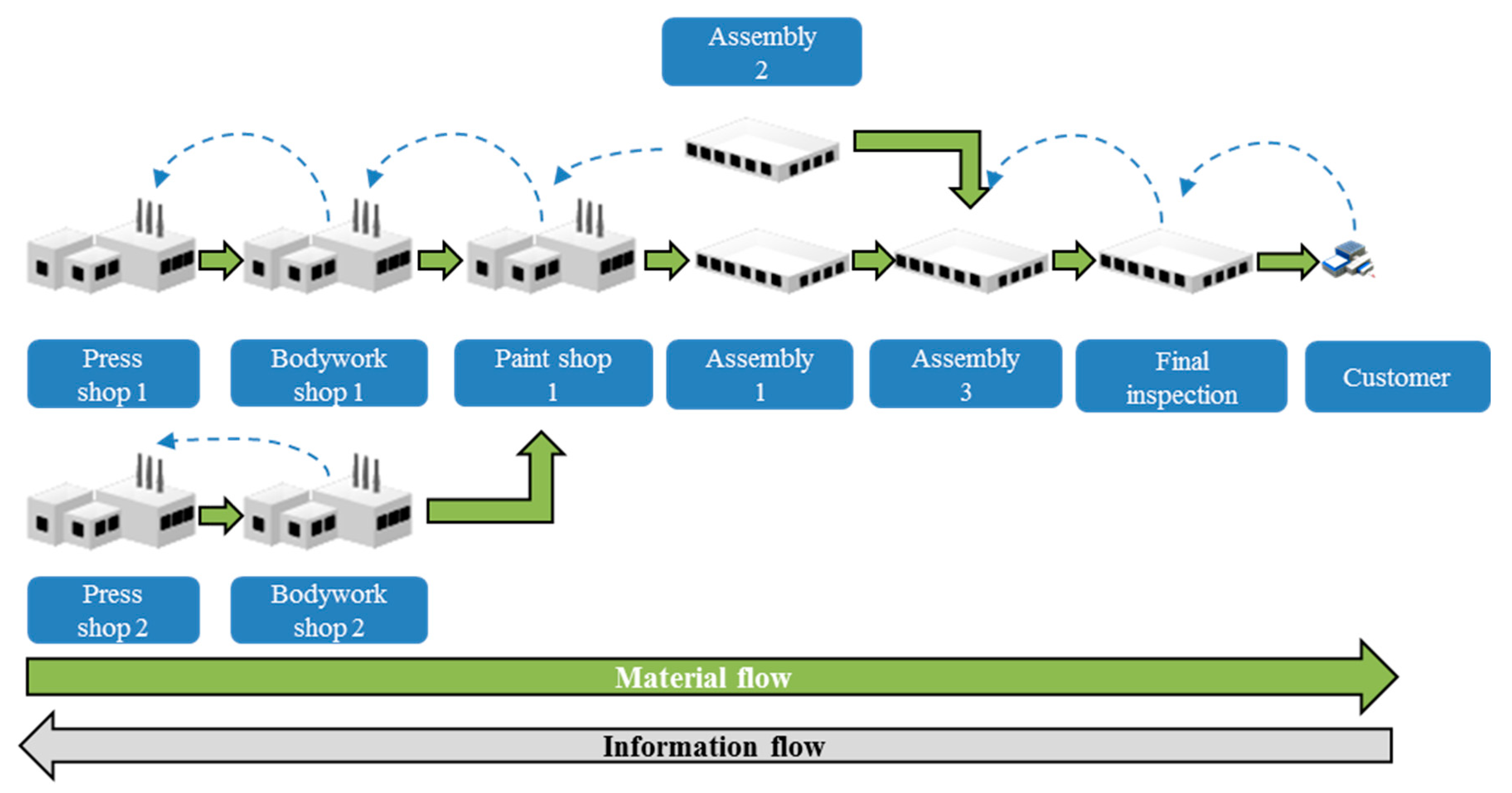
• Production consists of a process that begins with steel stamping and ends with final revision. The plants in the process are shown in Figure 3 and listed below.
• Press shop 1: a nominal capacity of 300 units per day.
• Bodywork shop 1: a nominal capacity of 300 units per day.
• Press shop 2: a nominal capacity of 300 units per day.
• Bodywork shop 2: a nominal capacity of 300 units per day.
• Paint shop: a nominal capacity of 600 units per day.
• Pre-assembly shop, assembly 1: a nominal capacity of 600 units per day.
• Mechanical assembly shop, assembly 2: a nominal capacity of 600 units per day.
• Final assembly shop, assembly 3: a nominal capacity of 600 units per day.
• Final inspection shop: a nominal capacity of 600 units per day.

As can be seen in Figure 3, the two car models use the same production capacity for the painting and assembly processes but use different capacities for the bodywork and press processes.

Four demand scenarios were simulated. In all scenarios, there are two products or car models with the same platform. The first model is at a mature stage in its life cycle, and the second model is newly launched with demand depicted in Figure 4. Demand was created in Excel in order to use replication to have exactly the same demand in all of the models. This method of data generation allowed us to create customized demand patterns to be read by Vensim. According to many authors, the basic demand patterns are steady, seasonal, trend, and sporadic demand patterns [16]. These demand patterns were applied in combination as a basis for demand in the models to describe the behavior of the simulation models.

For the four previously described scenarios and both simulation models, the following key performance indicators (KPIs) were calculated from the simulation:

• Profits (million euros): the result of the multiplication of the number of produced cars by the margin that was provided for the type of produced car.
• Total production (units): the cumulative sum of all car units produced over the 1000 simulated production days.
• Capacity utilization (%): the cumulative utilization of available capacities over the 1000 simulated production days.
• Maximum production capacity (units/day): both models were initialized with a demand of 600 units per day. This KPI shows the maximum capacity that was achieved during the simulated period.
• Service level (%): the quantity of units delivered on time divided by the total number of delivered units.
• Customer order lead time (days): the number of days between the placement of the order and the delivery of the product.
• Operational savings (million euros): the savings due to optimization of working hours, shifts, and maintenance activities.
• Investment value (million euros): the amount of the investment made to increase capacities. The value can be 30 million euros for an increase of up to 700 units per day or 60 million euros for an increase of up to 800 units per day.
• Return on investment (million euros): the margin of the products that can be produced thanks to the investment minus the investment value.

4.3. Simulation Results for the Case Study of an Automotive Plant

Before the results from the model were extracted and interpreted, a formal validation was performed. According to Sterman, there are 12 possible methods for validating system dynamics models [17]. There are three that are relevant to our models; one of them is the extreme-value test, which we used in this paper. An application of this method proved that the model’s response is plausible when taking extreme values for different input parameters. Some basic physical laws should be examined, for example, when there are no employees, the model’s output should not able to meet the demand. For both models, the same input and output variables were chosen in order to analyze and validate the models. These input variables are nominal capacity and customer demand. From the variation in these variables, the following can be expected in order for the results to be logical and the model to be validated:

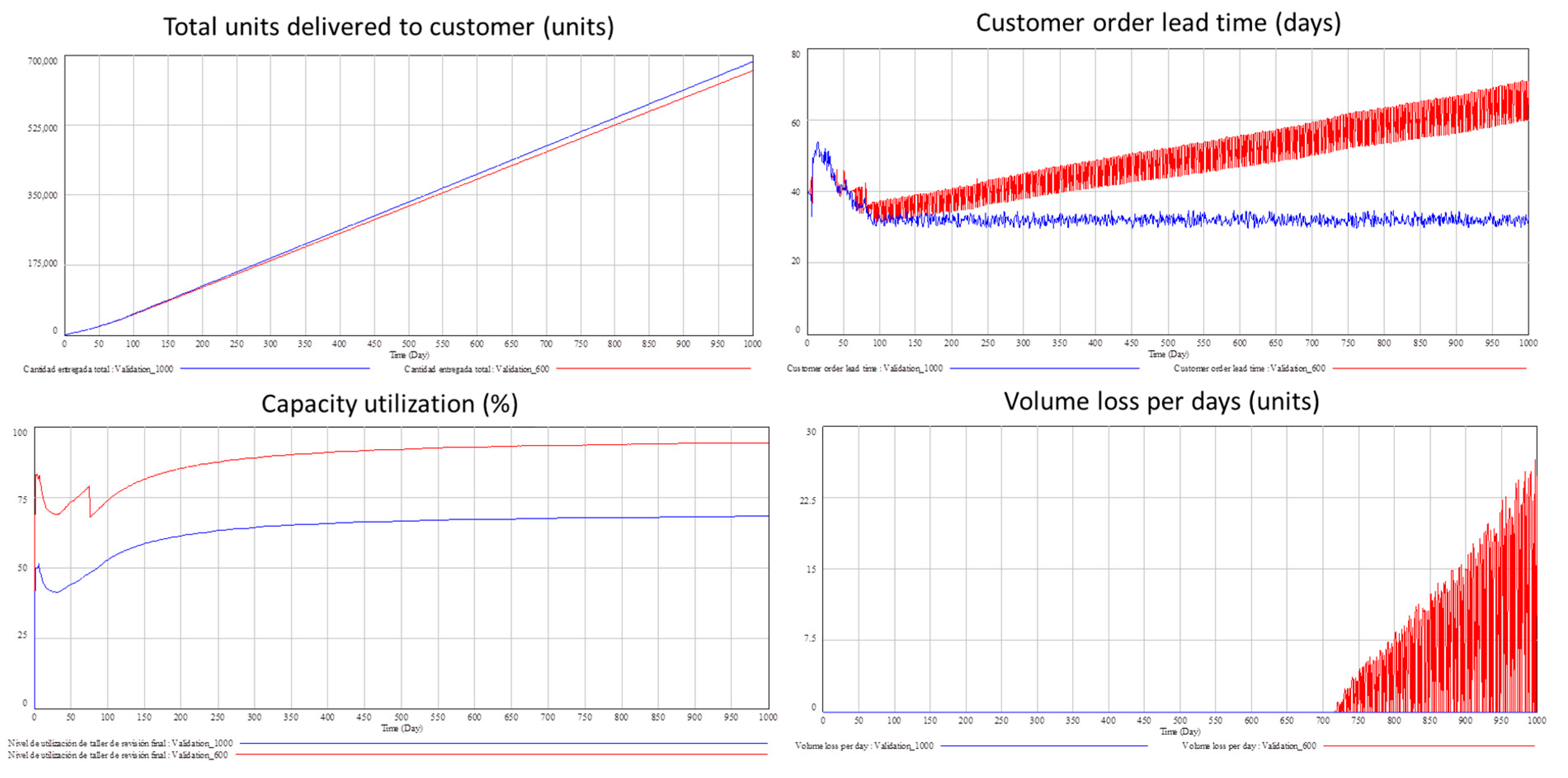
• For a lower nominal capacity (units per day), the customer order lead time, volume loss, and capacity utilization must be higher, and the total number of units delivered to customers must be lower, as shown in Figure 5. The red lines indicate the lower nominal capacity, and the blue ones indicate the higher nominal capacity.
• For a lower customer demand (units per day), the customer order lead time, volume loss, capacity utilization, and total number of units delivered to customers must be lower.

After the validation, the results for the four demand scenarios were extracted for the selected key performance indicators.

In the first scenario, the VSM produced better results for all relevant indicators as it can be seen in

Table 1. Simulation results for demand scenario 1, stationary scenario, at the plant level. VSM, viable system model.

Simulation Level	Demand Scenario 1	Key performance Indicator (KPI)	VSM Simulation Model	Nonviable Simulation Model
Plant level	- Launch curve until t = 100 days - Stationary demand for the new model at 400 units/day and for the 2nd model at 300 units/day	Profits (million euros)	1021	1012
		Total production (units)	660,129	655,761
		Capacity utilization (%)	94.3	82.0
		Maximum production capacity (units/day)	700	800
		Service level (%)	98.5	97.6
		Customer order lead time (days)	49.7	58.6
		Operational savings (million euros)	1.0	0.0
		Investment value (million euros)	30.0	60.0
		Return on investment (million euros)	70.0	70.0

, although the nonviable system model increased its capacity by 200 units per day. As this decision was made with a delay in comparison to the viable system model, the total number of delivered units was almost 5000 units lower and the capacity utilization was 12% lower.

Moreover, the viable system model generated a profit of 1021 million euros, whereas the nonviable system model generated a profit of 1012 million euros, which is nine million euros less. In addition, the VSM was able to generate savings of one million euros.

For both scenarios, the return on investment (ROI) was positive at the moment the decision was made. The value was the same; however, the VSM achieved this ROI with an investment value that was 30 million euros less due to a lower increase in capacities than the nonviable system model. As the decision was made later, the customer order lead time was almost 10 days longer in the nonviable system model.

Therefore, from the comparison of the models, the results show that the VSM would be selected as desirable in this demand scenario due to its combination of a low investment and a low cost and its highly efficient deployment (lead time, service level, and capacity utilization).

In the second scenario, the VSM also produced better results for all relevant indicators as shown in

Table 2. Simulation results for demand scenario 2, trend/stationary scenario, at the plant level. VSM, viable system model.

Simulation Level	Demand Scenario 2	Key Performance Indicator (KPI)	VSM Simulation Model	Nonviable Simulation Model
Plant level	- Trend until t = 250 days until stationary demand for the new model at 400 units/day and for the 2nd model at 300 units/day	Profits (million euros)	934	925
		Total production (units)	617,021	612,520
		Capacity utilization (%)	88.2	76.7
		Maximum production capacity (units/day)	700	800
		Service level (%)	97.2	95.3
		Customer order lead time (days)	46.3	54.4
		Operational savings (million euros)	3.5	0.0
		Investment value (million euros)	30.0	60.0
		Return on investment (million euros)	28.8	15.4

, although, as in the first scenario, the nonviable system model increased its capacity by 200 units per day. As this decision was made with a delay in comparison to the viable system model, the total number of delivered units was nearly 5000 units lower, and the capacity utilization was almost 12% lower.

Moreover, the viable system model generated a profit of 934 million euros, whereas the nonviable system model generated a profit of 925 million euros, which is nine million euros less. In addition, the VSM was able to generate savings of 3.5 million euros.

For both scenarios, the return on investment was positive at the moment the decision was made. The ROI in the VSM was 13.4 million euros higher than that in the nonviable system model and it was achieved with an investment that was 30 million euros less. Moreover, the customer order lead time was 8.1 days larger in the nonviable system model due to a long decision-making process that led to an investment to increase production by 200 units per day. The VSM model increased production by only 100 units per day.

Therefore, as in the first scenario, from the comparison of the models, the results show that the VSM simulation model would be selected as desirable in this demand scenario due to its combination of a low investment, operational savings, and highly efficient deployment (lead time, service level, and capacity utilization).

In the third scenario, according to

Table 3. Simulation results for demand scenario 3, trend scenario, at the plant level. VSM, viable system model.

Simulation Level	Demand Scenario 3	Key Performance Indicator (KPI)	VSM Simulation Model	Nonviable Simulation Model
Plant level	- Trend with slope +1.2 until t = 250, +0.2 until t = 750 and −0.4 until t = 1000 - Stationary demand for the 2nd model at 300 units/day	Profits (million euros)	887	794
		Total production (units)	593,280	546,885
		Capacity utilization (%)	84.8	91.2
		Maximum production capacity (units/day)	700	600
		Service level (%)	96.3	94.0
		Customer order lead time (days)	41.0	70.9
		Operational savings (million euros)	10.0	0.0
		Investment value (million euros)	30.0	0.0
		Return on investment (million euros)	70.0	-

, the VSM produced better results for all relevant indicators except capacity utilization due to the fact that the nonviable system model did not increase its capacity. As this decision was never made, the viable system model produced a higher total number of delivered units but lower capacity utilization. This situation arises from the fact that, as the demand was volatile and had a trend pattern, the nonviable system model was not able to identify the need for a new investment. This led to a volume loss of almost 45,000 units during the four-year period and a profit loss of 91 million euros. In addition, the VSM was able to generate savings of 10.0 million euros.

As the nonviable system model did not increase its capacity, the capacity utilization was 6.4% higher than in the VSM, which increased its capacity by 100 units per day. The return on investment of this increase is positive and accounts for 70 million euros. Moreover, the customer order lead time in the nonviable system model was almost 30 days longer than in the VSM model. In addition, the service level was also 2.3% higher in the VSM model.

Therefore, from the comparison of the models, the results show that the VSM would be selected as desirable in this demand scenario due to the investment made, the savings achieved, and its highly efficient deployment (lead time, service level, and capacity utilization), thanks to an anticipated investment that the nonviable model did not decide to make.

In the last scenario, as shown in

Table 4. Simulation results for demand scenario 4, seasonal scenario, at the plant level. VSM, viable system model.

Simulation Level	Demand Scenario 4	Key Performance Indicator (KPI)	VSM Simulation Model	Nonviable Simulation Model
Plant level	- Launch curve until t = 100 days - Seasonal demand for the new model at 350 units/day, and stationary for the 2nd model at 300 units/day	Profits (million euros)	935	842
		Total production (units)	617.390	565.968
		Capacity utilization (%)	88.2	94.3
		Maximum production capacity (units/day)	700	600
		Service level (%)	97.9	91.8
		Customer order lead time (days)	44.2	88.2
		Operational savings (million euros)	12.5	0.0
		Investment value (million euros)	30.0	0.0
		Return on investment (million euros)	20.4	-

, the VSM produced better results for all relevant indicators except capacity utilization due to the fact that the nonviable system model did not increase its capacity. As this decision was never made, the viable system model produced a higher total number of delivered units but lower capacity utilization. This situation arises from the fact that, as the demand was volatile and had a seasonal pattern, the nonviable system model was not able to identify the need for a new investment. This led to a volume loss of more than 51,000 units during the four-year period and a profit loss of 93 million euros. In addition, the VSM was able to generate savings of 12.5 million euros.

As the nonviable system model did not increase its capacity, the capacity utilization was 6.1% higher than in the VSM, which increased its capacity by 100 units per day. The return on investment of this increase was positive and accounted for 20.4 million euros. Moreover, the customer order lead time in the nonviable system model was 40 days longer than in the VSM model. In addition, the service level was also 6.1% higher in the VSM model.

Therefore, from the comparison of the models, the results show that the VSM would be selected as desirable in this demand scenario due to the investment made, the savings achieved, and its highly efficient deployment (lead time, service level, and capacity utilization), thanks to an anticipated investment that the nonviable model did not decide to make.

5. Conclusions

As a result of the research work, the main hypothesis was supported based on the following facts:

• Thanks to a new conceptual model for capacity planning able to make decisions for reduction or increase of production capacity, the viability of a company can be assured. As a result, it proves the need for such a system as a standard tool for managers in the future in order to increase the efficiency and adaptability of manufacturing organizations.
• The viable system model provides the necessary structure to determine the interrelationships among areas and parameters that allow decisions to be made regarding capacity in an autonomous process based on selected control limits.
• The simulation of an OEM plant using the developed conceptual model presents better results compared with currently available structures regarding how to deal with customer demand volatility.

The final goal is to transfer this research method to real production systems, where it could be applied in particular cases as a tool to assist managers by centralizing all data related to a topic in a short period of time, enabling the simulation of what-if scenarios, and speeding up decision-making processes as a unique selling proposition (USP) of manufacturing organizations.

The results show the benefits of capacity management based on a digital-twin approach in which top management can make decisions in a short period of time. However, the question of how it can be made possible in large organizations involving multiple plants and departments remains to be answered.

Future research could develop a virtual model of a manufacturing organization by including other decision-making factors and determine how these decisions and approaches could be realized in the real world with current technologies and systems.

References

1. Kühnapfel, J.B. Vertriebsprognosen. In Vertriebscontrolling; Springer Gabler: Wiesbaden, Germany, 2014. [Google Scholar]
2. Stadtler, H.; Kilger, C. Supply Chain Management and Advanced Planning; Springer: Berlin, Germany, 2002–2005; Volume 4, p. 139. [Google Scholar]
3. Schuh, G.; Stich, V.; Wienholdt, H. Logistikmanagement; Springer Vieweg: Berlin, Germany, 2013; p. 89. [Google Scholar]
4. Campuzano, F.; Mula, J. Supply Chain Simulation: A System Dynamics Approach for Improving Performance; Springer Science & Business Media: Berlin, Germany, 2011; p. 23. [Google Scholar]
5. Schönsleben, P. Integrales Logistikmanagement: Operations and Supply Chain Management in Umfassenden Wertschöpfungsnetzwerken; Springer: Berlin, Germany, 2011; p. 668. [Google Scholar]
6. Frazelle, E. Supply Chain Strategy: The Logistics of Supply Chain Management; McGraw Hill: New York, NY, USA, 2002; p. 117. [Google Scholar]
7. Gupta, M.C.; Boyd, L.H. Theory of constraints: A theory for operations management. Int. J. Oper. Prod. Manag. 2008, 28, 991–1012. [Google Scholar] [CrossRef]
8. Beschaffungsmanagement Revue De L’acheteur; Verein procure.ch: Aarau, Switzerland, 2010; Volume 10/10, pp. 16–17.
9. Biedermann, H. Ersatzteilmanagement: Effiziente Ersatzteillogistik Für Industrieunternehmen; Springer: Berlin, Germany, 2008. [Google Scholar]
10. Espejo, R.; Harnden, R. The Viable System Model: Interpretations and Applications of Stafford Beer’s VSM; Wiley: Hoboken, NJ, USA, 1989. [Google Scholar]
11. Auerbach, T.; Bauhoff, F.; Beckers, M.; Behnen, D.; Brecher, C.; Brosze, T.; Esser, M. Selbstoptimierende produktionssysteme. In Integrative Produktionstechnik Für Hochlohnländer; Springer: Berlin, Germany, 2011; pp. 747–1057. [Google Scholar]
12. Schuh, G.; Stich, V.; Brosze, T.; Fuchs, S.; Pulz, C.; Quick, J.; Bauhoff, F. High resolution supply chain management: Optimized processes based on self-optimizing control loops and real time data. Prod. Eng. 2011, 5, 433–442. [Google Scholar] [CrossRef]
13. Beer, S. Brain of the Firm: A Development in Management Cybernetics Herder and Herder; Verlag Herder: Freiburg im Breisgau, Germany, 1972. [Google Scholar]
14. Coyle, R.G. System Dynamics Modelling: A Practical Approach; Chapman & Hall: London, UK, 2008. [Google Scholar]
15. Schuh, G.; Stich, V. Logistikmanagement. 2., vollständig neu bearbeitete und erw. Auflage; 2013. [Google Scholar]
16. Meyer, J.C.; Sander, U.; Wetzchewald, P. Bestände Senken, Lieferservice Steigern-Ansatzpunkt Bestandsmanagement; FIR: Aachen, Germany, 2019. [Google Scholar]
17. Wensing, T. Periodic Review Inventory Systems; Springer: Berlin, Germany, 2011; Volume 651. [Google Scholar]
Figure 1. Recursion levels of the conceptual model and capacity management at the plant level based on the viable system model.
Applsci 09 05567 g001
Figure 2. Use suitability of forecasting methods [15].
Applsci 09 05567 g002
Figure 3. Simulation production flow (own elaboration).
Applsci 09 05567 g003
Figure 4. The four demand scenarios for the new car model (own elaboration).
Applsci 09 05567 g004
Figure 5. Results of the validation for nominal capacity using the extreme-value test (own elaboration).
Applsci 09 05567 g005