A Hybrid Machine Learning and Population Knowledge Mining Method to Minimize Makespan and Total Tardiness of Multi-Variety Products

Abstract

Nowadays, the production model of many enterprises is multi-variety customized production, and the makespan and total tardiness are the main metrics for enterprises to make production plans. This requires us to develop a more effective production plan promptly with limited resources. Previous research focuses on dispatching rules and algorithms, but the application of the knowledge mining method for multi-variety products is limited. In this paper, a hybrid machine learning and population knowledge mining method to minimize makespan and total tardiness for multi-variety products is proposed. First, through offline machine learning and data mining, attributes of operations are selected to mine the initial population knowledge. Second, an addition–deletion sorting method (ADSM) is proposed to reprioritize operations and then form the rule-based initial population. Finally, the nondominated sorting genetic algorithm II (NSGA-II) hybrid with simulated annealing is used to obtain the Pareto solutions. To evaluate the effectiveness of the proposed method, three other types of initial populations were considered under different iterations and population sizes. The experimental results demonstrate that the new approach has a good performance in solving the multi-variety production planning problems, whether it is the function value or the performance metric of the acquired Pareto solutions.

1. Introduction

In recent years, digital integration and artificial intelligence have accelerated at an explosive rate. This progress inevitably leads to the rapid development of two technologies: big data [1,2,3] and intelligent algorithms [4]. For enterprise production planning or scheduling, although there are many machine learning algorithms [5,6,7,8,9] for this problem, there are still not many data mining methods, especially for multi-objective job shop scheduling problems (MOJSSP) [10].

MOJSSP is an important and critical problem for today’s enterprises. A MOJSSP model can typically be described as a set of machines and jobs under multiple objectives, where each job has different sequential operations and each job should be processed on machines in a given order. This pattern is in line with the production planning problem for multi-variety products with different routings. Herein, the problem is transformed into how to rationally arrange the order of operations of multi-variety products on various machine tools, such that two or more objectives are optimal, e.g., makespan and total tardiness.

The characteristics of multi-objective problems increase the computational difficulty of traditional single-objective scheduling, while data mining [11] could extract rules from a large dataset without too much professional scheduling knowledge, which has more research space in solving MOJSSP and obtaining the optimal values of the objectives.

For the benefits of data mining, a multi-objective production planning method combining machine learning and population knowledge mining is proposed. Through the relation hierarchies mapping [12], attributes related to processing time and due date are selected. The machine learning algorithm used here is a hybrid metaheuristic algorithm that combines nondominated sorting genetic algorithm II (NSGA-II) and simulated annealing. It provides training data for the mining of population knowledge, and the rules obtained can be used as the criterion for sorting operations. Each operation gets its priority through rules, but it sometimes fails to meet the requirements of the rules (the number of operations per priority is fixed). Besides, the sequence of operations should also be considered. Therefore, this paper proposes a comprehensive priority assignment procedure called addition–deletion sorting method (ADSM) which can meet not only the optimized priority but also the requirements of rules and the order of operations. The main contributions of this paper are highlighted as follows:

(1)

A hybrid machine learning and population knowledge mining method is proposed to solve multi-objective job shop scheduling problems.

(2)

Five attributes, namely operation feature, processing time, remaining time, due date, and priorities, are selected to mine initial population knowledge.

(3)

The ADSM method is designed to reprioritize operations after the population knowledge mining.

(4)

Three populations (rules, mixed, and random) with different iterations and population sizes are compared, and three performance metrics are defined to explore the effectiveness of the proposed method.

2. Literature Review

MOJSSP is increasingly attracting scholars and researchers. Most methods are based on a multi-objective evolutionary algorithm (MOEA) [13], which first generates an initial population of production planning and then iterates continuously to obtain the best results. Huang [14] proposed a hybrid genetic algorithm to solve the scheduling problem while considering transportation time. Souier et al. [15] used NSGA-II for real-time scheduling under uncertainty and reliability constraints. Ahmadi et al. [16] used NSGA-II and non-dominated ranking genetic algorithm (NRGA) to optimize the makespan and stability under the disturbance of machine breakdown. Zhou et al. [17] presented a cooperative coevolution genetic programming with two sub-populations to generate scheduling policies. Zhang et al. [18] utilized a genetic algorithm combined with enhanced local search to solve the energy-efficiency job shop scheduling problems. A high-dimensional multi-objective optimization method was proposed by Du et al. [19]. To improve the robustness of scheduling, constrained nondominated sorting differential evolution based on decision variable classification is developed to acquire the ideal set.

In addition to the MOEA method, there are many other approaches to solve MOJSSP. Sheikhalishahi et al. [20] studied the multi-objective particle swarm optimization method. In their paper, makespan, human error, and machine availability are considered. Lu et al. [21] employed a cellular grey wolf optimizer (GWO) for the multi-objective scheduling problem with the objectives of noise and energy, while Qin et al. [22] tried to overcome the premature convergence of the GWO in solving MOJSSP by combining an improved tabu search algorithm. Zhou et al. [23] proposed three agent-based hyper-heuristics to solve scheduling policies with constrains of dynamic events. Fu et al. [24] designed a multi-objective brain storm optimization algorithm to minimize the total tardiness and energy consumption. Their goal is to minimize multiple objectives through MOEA or other metaheuristic algorithms, without exploiting a data mining method to improve the performance of scheduling.

With the development of industrial intelligence, data mining could be applied to management analysis and knowledge extraction. For MOJSSP, it could play a key role to solve the scheduling problem in the future. Recently, some researchers are trying to apply data mining to overcome the difficulties of job shop scheduling problems. Ingimundardottir and Runarsson [25] used imitation learning to discover dispatching rules. Li and Olafsson [26] introduced a method for generating scheduling rules using the decision tree. In their research, data mining extracts the rules that the attributes of jobs determine which one is better to be processed first. Similarly, Olafsson and Li [27] applied a decision tree to learn directly from scheduling data where the selected instances are identified as preferred training data. Jun et al. [28] proposed a random-forest-based approach to extract dispatching rules from the best schedules. This approach includes schedule generation, rule learning, and discretization such that they could minimize the average total weighted tardiness for job shop scheduling. Kumar and Rao [29] applied data mining to extract patterns in data generated by the ant colony algorithm, which generate a rule set scheduler that approximates the ant colony algorithm’s scheduler. Nasiri et al. [30] gained a rule-based initial population via GES/TS method, and then employed PSO and GA to verify the advantage of this method, but lacked the consideration of operations sequence. Most of them considered data mining as a tool to extract dispatching rules, while only a few of them utilized a data mining approach to generate the initial population of metaheuristic methods, not to mention multi-objective job shop scheduling problem.

This paper uses data mining to generate the rule-based initial population for MOJSSP. The operation sequence is considered and an addition–deletion sorting method is presented to reprioritize the order of operations of each job. The advantage of the proposed method is reflected by the NSGA-II with simulated annealing method of the random initial population under different criteria of iteration numbers and different initial population sizes.

3. Problem Description and Goal

The MOJSSP can be described as n jobs {J₀, J₁, …, J_n} under multiple objectives processed on m machines {M₀, M₁, …, M_m} with different routes [31]. The processing order of each part and the processing time of each operation o_ij on a machine is determined. To illustrate the problem, the encoding of a benchmark of 10 × 10 job shop (LA18) [32] here can take an example as {9, 8, 5, 4, 2, 1, 3, 6, 7, 0, …,5, 8, 9}. Each element in the operation sequence code represents a job. The ith occurrence of the same value means the ith operation of this job. Here, the MOJSSP aims to find an order to optimize the above two objectives simultaneously. The constraints include each job should be processed on only one machine at a time, each machine can process only one job at a time, and the preemption is not allowed [33].

Notations used are listed below:

i, h: index of jobs, i, h ∈ {0, 1, 2, …, n}

j, l: index of operations in a given job, j, l ∈ {0, 1, 2, …, o}

k, g: index of machines, k, g ∈ {0, 1, 2, …, m}

m: number of machines

n: number of jobs

o: number of operations in a given job

o_ij: the jth operation of the job i

C_i: the completion time of the job i

T_ijk: the processing time of the jth operation of the job i on machine M_k

E_ijk the completion time of the jth operation of the job i on machine M_k

D_i: the due date of the ith job

M_ij: set of available machines for the jth operation of job i

Index:

$$X_{ijk}=\left\{\begin{array}{l}1,\mathrm{if}{o}_{ij}\mathrm{is}\mathrm{machined}\mathrm{on}{M}_k\\ 0,\mathrm{otherwise}\end{array}\right\}$$

Two objective functions are simultaneously minimized:

$$\min \mathrm{F}1=\max \left\{C_i\right|i=0,1,\dots ,n\}$$

(1)

$$\mathrm{F}2={\displaystyle \sum _{i=0}^n(C_i-D_i)}$$

(2)

Subject to:

$$E_{ijk}>0,i=0,1,\dots ,n;j=0,1,\dots o;k=0,1,\dots ,m$$

(3)

$$E_{i(j+1)g}-E_{ijk}\ge X_{i(j+1)g}\times T_{i(j+1)g},i=0,1,\dots ,n;j=0,1,\dots ,o-1;k,g=0,1,\dots ,m$$

(4)

$$E_{ijk}-E_{hlk}\ge X_{ijk}\times T_{ijk}\mathrm{or}{E}_{hlk}-E_{ijk}\ge X_{hlk}\times T_{hlk},i=0,1,\dots ,n;j=0,1,\dots ,o;k=0,1,\dots ,m$$

(5)

$${\displaystyle \sum _{j=0}^o{X}_{ijk}=1,i=0,1,\dots ,n;k=0,1,\dots ,m}$$

(6)

Equations (1) and (2) are used to minimize the makespan (F1) and total tardiness (F2), respectively. Equation (3) is the variable restriction. Equation (4) ensures the sequence of operations. Equation (5) is used to constrain operations so that they do not overlap. Equation (6) indicates an operation of a job could only be processed on one machine, that is, an operation cannot be divided, and it can only be processed on one machine from the beginning to completion.

4. The Hybrid Machine Learning and Population Knowledge Mining Method

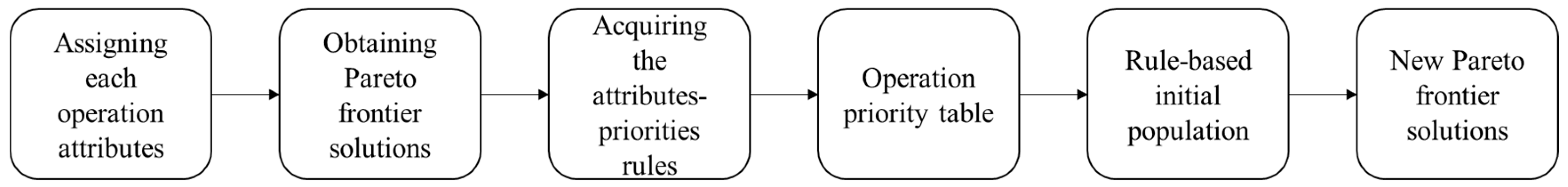
The main process of the approach for MOJSSP (PAMOJSSP) is briefly illustrated in Figure 1. The process is started from the operations’ attributes assignment. In this step, the attributes of each operation are deduced from the optimized objective functions, corresponding to the process information of each operation. These attributes’ information is embedded into the individual class and then, under the calculation of metaheuristic algorithm, the Pareto frontier solutions presented as the optimal results among these non-dominated solutions are obtained. This series of Pareto frontier can be used as training data to obtain potential rules in these non-dominated solutions through data mining. After the acquisition of rules, an operation priority table is obtained by the rule correspondence and the ADSM. The rule-based initial population is eventually acquired by crossing the genes of the parent individual in the operation priority table. In the last step, the rule-based initial population combined with the hybrid metaheuristic algorithm obtains the new better Pareto frontier solutions for MOJSSP.

The following part introduces the concrete implementation of the proposed method.

4.1. Attributes

On the basis of attribute-oriented induction [34], combined with the optimization objectives of this problem, five attributes are finally determined: priority, operation feature, processing time, remaining time, and due date. Each attribute is classified into two or more types and explained in the following subsections.

4.1.1. Priorities

Priorities mean the position of each operation in the final sequence code. From the benchmark of 10 × 10 job shop problem, 100 positions could be acquired and needed to be sequenced to optimize the makespan and total tardiness. Ten classes of priorities are divided, and each priority has ten positions. That is, we divide the operation sequence code into 10 equal parts from front to back, with the priority of 0, 1, 2, …, 9, respectively. The number 0 indicates the highest priority level, while number 9 indicates the lowest priority level.

4.1.2. Operation Feature

Operation feature means the position of each operation in its route process. Referring to Nasiri et al. [30], the first operation is classified as “first”. The second and third operations are labeled with “secondary”. The fourth, fifth and sixth operations are classified as “middle”. The seventh, eighth, and ninth operations mean “later”. Finally, the tenth is labeled with “last”.

4.1.3. Processing Time

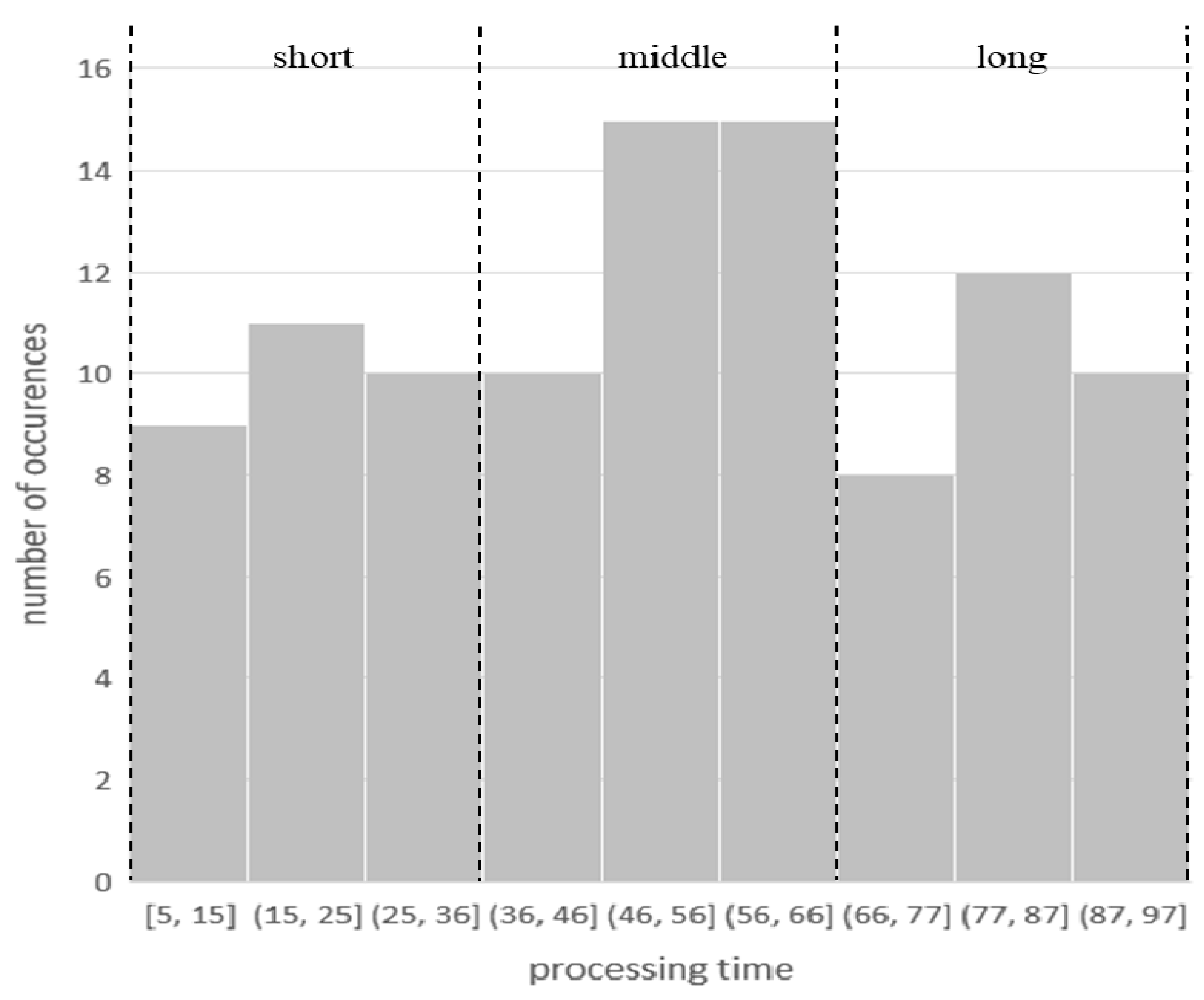
Processing time is the required processing time for each operation on its predetermined machine. For LA18, we classified the processing time into three equal part as “short”, “middle”, and “long”. As illustrated in Figure 2, the processing time with less than 37 is classified as “short”. The time between 37 and 67 is “middle” and the left time is labeled with “long”.

4.1.4. Remaining Time

Remaining time refers to the accumulative processing time for the remaining operations to be processed after the current operation. As with the classification of processing time, its histogram is shown in Figure 3. The remaining time with less than 202 is defined as “short”, the time between 202 and 402 is classified as “middle”, and the time with more than 402 is labeled as “long”.

4.1.5. Due Date

Due date is the time when a job must be delivered. For optimizing the total tardiness, it is a critical attribute which needs to be considered as an important input of data mining. Because the benchmark LA18 only provides the processing time information, here we add the due date for each job. According to the benchmark, the shortest makespan is 848. Therefore, we could set the due date of Jobs 0–9 as a random number from 1100 to 1290 and arrange them in order. The due date for Job 0 is the most urgent and the due dates of the remaining jobs increase in order, which means that the due dates for jobs become looser.

Table 1. Due date attribute.

Job No.	Due Date	Class
0	1100	tight
1	1150	tight
2	1150	tight
3	1180	tight
4	1180	tight
5	1200	slack
6	1200	slack
7	1250	slack
8	1250	slack
9	1290	slack

shows the values of due date attribute for jobs.

4.2. Data Preparation

First, the operation feature, processing time, remaining time, and due date of each operation in LA18 are matched one by one using the above methods.

Table 2. Samples of partial data for operation attributes.

Operation	Machine	Processing Time	Remaining Time	Operation Feature	Processing Time	Remaining Time	Due Date
00	6	54	507	first	middle	long	tight
01	0	87	420	secondary	long	long	tight
02	4	48	372	secondary	middle	middle	tight
03	3	60	312	middle	middle	middle	tight
04	7	39	273	middle	middle	middle	tight
05	8	35	238	middle	short	middle	tight
…	…	…	…	…	…	…	…
97	9	85	105	later	long	short	slack
98	5	46	59	later	middle	short	slack
99	0	59	0	last	middle	short	slack

lists some of its sample data. The difference of attributes can be obtained by the significant test (α = 0.05) [35]. The null hypothesis is that the significant difference of each column (each attribute) does not exist. The number of samples before matching is 100, while the p-value is 0.000, which is much less than 0.05. That is, the difference between columns is significant. After this, in the 9088 datasets obtained by 30 independent runs of NSGA-II combined with simulated annealing, 6645 non-dominated solutions were obtained after removing the repeated solutions. Among them, 493 sets of Pareto frontier solutions were obtained, and 66 sets of solutions were finally selected for the computational complexity, which forms 6600 transactions in a relational database.

Table 3. Sample data of the trained data.

ID	Operation	Operation Feature	Processing Time	Remaining Time	Due Date	Priority
0	40	first	long	middle	tight	0
1	40	first	long	middle	tight	0
2	90	first	middle	long	slack	0
3	90	first	middle	long	slack	0
4	90	first	middle	long	slack	0
5	40	first	long	middle	tight	0
6	40	first	long	middle	tight	0
7	80	first	short	long	slack	0
8	80	first	short	long	slack	0
9	00	first	middle	long	tight	0
…	…	…	…	…	…	…
6594	99	last	middle	short	slack	9
6595	79	last	middle	Short	slack	9
6596	99	last	middle	short	slack	9
6597	89	last	short	short	slack	9
6598	69	last	long	short	slack	9
6599	69	last	long	short	slack	9

shows the sample data of the trained data.

4.3. Rule Mining

Rule mining refers to mining association rules between attribute set {operation feature, processing time, remaining time, due date} and attribute {priority}. The decision tree is an effective means of mining classification. Here, we can get 33 rules from the theory of entropy, which is shown in Supplementary Materials File S1. However, the mined rules may have different priorities for the same attribute set. To discriminate this difference and enhance the richness of excellent populations, the weight of a priority class [12] in this paper is used to mine the rules behind the training data. The minimum value of the weight we set here is 0.01, which is the lower bound of the weight of the priority class. When the weight of a rule set under a priority class is less than this value, the rule set is considered not to belong to the priority class. The obtained 37 dominant rules are shown in

Table 4. Dominant rules obtained from knowledge mining.

Id	Rule Set	Priority
		0	1	2	3	4	5	6	7	8	9
0	first long long slack	0.67	0.15	0.14	0.05
1	first long middle tight	0.80	0.20
2	first middle long slack	0.71	0.28	0.01
3	first middle long tight	0.98	0.02
4	first middle middle tight	0.82	0.18
5	first short long slack	1.00
6	first short long tight	0.33	0.48	0.12	0.07
7	last long short slack						0.02	0.01	0.09	0.11	0.78
8	last long short tight						0.08	0.76	0.17	0.00	0.00
9	last middle short slack							0.07	0.02	0.17	0.75
10	last middle short tight							0.08	0.21	0.39	0.32
11	last short short slack								0.03	0.27	0.70
12	last short short tight						0.06	0.16	0.02	0.14	0.63
13	later long short slack				0.01	0.08	0.09	0.06	0.19	0.39	0.19
14	later long short tight					0.12	0.13	0.16	0.29	0.13	0.18
15	later middle middle slack				0.05	0.26	0.05	0.26	0.39
16	later middle short slack						0.12	0.18	0.27	0.24	0.19
17	later middle short tight				0.01	0.06	0.08	0.17	0.13	0.43	0.12
18	later short short slack					0.05	0.13	0.12	0.18	0.37	0.15
19	later short short tight					0.18	0.53	0.10	0.15	0.04
20	middle long middle slack		0.01	0.16	0.24	0.24	0.14	0.13	0.07
21	middle long middle tight			0.14	0.37	0.04	0.08	0.36	0.02
22	middle long short tight			0.05	0.27	0.40	0.21		0.08
23	middle middle middle slack			0.01	0.19	0.22	0.13	0.17	0.14	0.11	0.02
24	middle middle middle tight		0.02	0.24	0.39	0.26	0.09
25	middle middle short tight				0.30	0.36	0.15	0.18
26	middle short middle slack			0.14	0.14	0.52	0.14	0.07
27	middle short middle tight		0.07	0.18	0.15	0.11	0.08	0.22	0.17	0.02
28	middle short short slack					0.18	0.26	0.03	0.48	0.05
29	middle short short tight				0.36	0.12	0.30	0.06	0.15
30	secondary long long slack	0.03	0.62	0.17	0.05	0.04	0.05	0.05	0.01
31	secondary long long tight	0.03	0.82	0.15
32	secondary middle long slack	0.38	0.39	0.22	0.02
33	secondary middle middle slack		0.14	0.39	0.30	0.02	0.06	0.04	0.06
34	secondary middle middle tight	0.11	0.23	0.34	0.21	0.08	0.03	0.01
35	secondary short long slack	0.38	0.42	0.20
36	secondary short middle tight	0.18	0.33	0.39	0.10

.

The rules also could be expressed in the form of “if-then”. For example, Rule 3 is given as:

If (operation feature = “first”, and processing time = “middle”, and remaining time = “long”, and due date = “slack”)

Then, (priority = “0”, weight = “0.71”; priority = “1”, weight = “0.28”; priority = “2”, weight = “0.01”)

It should be mentioned that there may be a case where the sum of weights is not equal to 1, which is due to rounding and does not affect the results of rules.

4.4. Initial Population Generated Using ADSM

In this section, a rule-based initial population is finally obtained through the proposed ADSM. First, each operation obtains its possible position according to the mined rules. For example, from Table 2, attributes of Operation 00 are first, middle, long, and tight, which are consistent with the rule set with ID 3 in Table 4. It means that the priority weight of the first operation of the Job 0 is {priority = 0, weight = 0.98; priority = 1, weight = 0.02}. The highest priority level is initially defined as the possible position of the operation. Therefore, the initial priority of Operation 00 is 0. In Supplementary Materials File S2, these maximum values are labeled and all other priority weights can be obtained by traversing all operations. Next, the operations in each priority are readjusted to satisfy the requirement of ten operations per priority. To gain this purpose, ADSM is proposed to overcome problems that may arise during the sorting process.

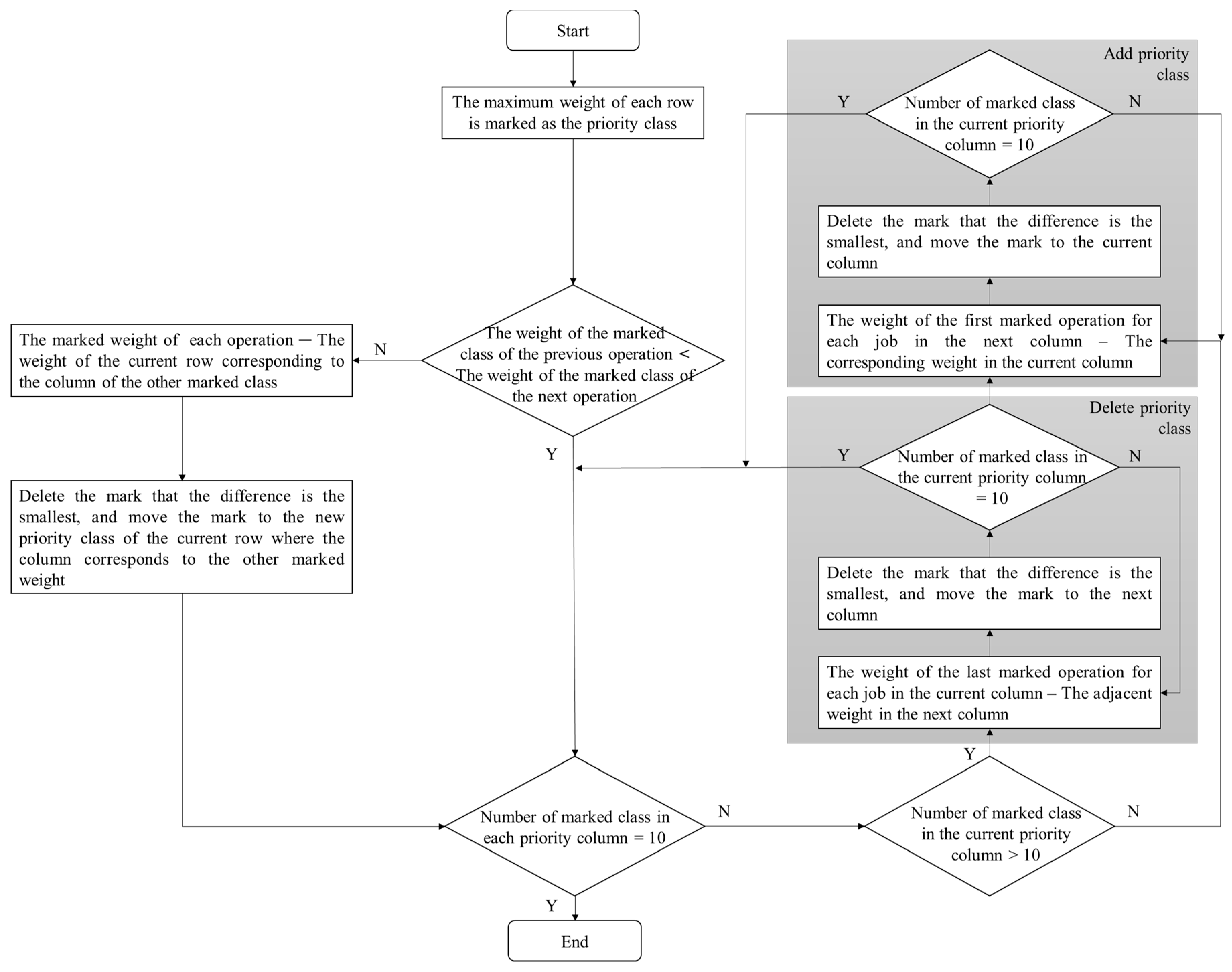
As shown in Figure 4, we define the marked weight as the priority class of each operation. In the process, there are three main situations. The first situation is that the priority order of operations may be incorrect because operations are processed sequentially. That is, the weight of the marked class of the previous operation may be higher than the next operation. While confronting this problem, these two marked weights of the operations should be compared. Through calculating the difference between the marked weight of each operation and the weight of the current row corresponding to the column of the other marked class, the smaller one should remove the mark from the current weight to the new weight of the current row where the column corresponds to the other marked weight.

After adjusting the order of all operations, the next problem is to assign the operations between each adjacent priority group to meet the requirement of ten operations per priority. There are two situations, namely “>10” and “<10”, which are the remaining two situations mentioned above. The second situation (the number of marked class in the current priority column >10) takes the deletion sorting method, that is removing the extra marked weights to the next priority column. The mark with the smallest difference is removed, which here refers to the difference between the weight of the last marked operation for each job in the current column and the adjacent weight in the next priority column. In the third situation (the number of marked class in the current priority column <10), the addition sorting method is used to add marked classes from the next priority column to the current priority column. The mark with the smallest difference is added first, and the standard is the difference between the weight of the first marked operation for each job in the next column and the corresponding weight in the current priority column. In the cases that the minimum difference is the same, the deletion sorting method first removes the marked operations with the higher encoded number, while the addition sorting method first provides the marked operations with the smaller encoded number.

5. Experiment

The proposed method was applied to a well-known multi-objective metaheuristic algorithm, which runs 10 times per calculation in Eclipse. To better explain this method, a rule-based initial population and a mixed initial population mined by this method were compared with the random population under different criteria based on the benchmark LA18.

5.1. Selected Algorithm

For the multi-objective scheduling problem, the most popular algorithm is NSGA-II. However, it lacks a better local search capability. It means that, when solving some cases, its results usually fall into a locally optimal solution. To make experimental results more accurate and better, this study used the NSGA-II combined with simulated annealing (SA). The following introduces the NSGA-II and SA algorithm and the parameters used.

• Nondominated sorting genetic algorithm II (NSGA-II)
    Based on NSGA, developed by Deb et al. [36], NSGA-II has the advantage of fast running speed, good robustness, and fast convergence. The encoding method is consistent with the above described. Each gene means an operation. Each chromosome/individual represents a solution or a sequence of all the operations waiting to be scheduled. NSGA-II combines parent and offspring into a new population and then obtains the non-dominated solutions by fast non-dominated sorting. The parent is generated by disrupting genes in the chromosome. The offspring is generated by the crossover and mutation method. The parameters are shown in

  Table 5. Parameters used in NSGA-II.

  Parameters	Values
  population size	25, 50, 100
  mutation rate	0.002
  crossover rate	0.9
  size of tournament selection	10
  number of iterations	100, 300

  .
• Simulated annealing (SA)
    Simulated annealing is an approximate method based on Monte Carlo design. It was first introduced by Kirkpatrick et al. [37] to solve the optimization problem. SA accepts a solution that is worse than the current solution by the Metropolis criterion, thus it is possible to jump out of this local optimal solution to reach the global optimal solution.

  Table 6. Parameters used in SA.

  Parameters	Values
  population size	25, 50, 100
  initial temperature	100
  end temperature	0.01
  cooling rate	0.001
  number of iterations	100, 300

  lists the parameters used in SA.

The non-dominated solutions were obtained by NSGA-II, and then SA was used to local search. Because of the multi-objective reasons, an objective function was randomly selected as the direction of a search, and the obtained non-dominated solutions were stored in the external archive. SA was applied to local search every 50 generations in this experiment.

To obtain better initial population rules, the data source of data mining must be the optimal or near-optimal solution set, so that accurate and reliable rules can be discovered. In

Table 7. Makespan of the NSGA-II and NSGA-II + SA.

IP	IT		NSGA-II	NSGA-II + SA
25	100	best	933	853
		average	974	909
	300	best	895	848
		average	947	910
50	100	best	895	854
		average	941	912
	300	best	865	848
		average	931	915
100	100	best	898	848
		average	938	919
	300	best	861	848
		average	912	943

and

Table 8. Total tardiness of the NSGA-II and NSGA-II + SA.

IP	IT		NSGA-II	NSGA-II + SA
25	100	best	−3860	−4529
		average	−3350	−4338
	300	best	−4001	−4524
		average	−3757	−4537
50	100	best	−4241	−4630
		average	−3743	−4400
	300	best	−4279	−4815
		average	−3982	−4569
100	100	best	−4273	−4698
		average	−3703	−4495
	300	best	−4539	−4698
		average	−4229	−4587

, we can see that the data obtained by NSGA-II hybrid with SA are more effective, thus the results obtained by this algorithm were selected as the data source of knowledge mining. More comparisons between this algorithm and other algorithms can be seen in [38].

To verify the knowledge mining method, three different initial populations of NSGA-II combined with simulated annealing were considered as follows:

• Knowledge mining heuristic optimization method (rule)
  The initial population was generated using the proposed hybrid machine learning and population knowledge mining method.
• Heuristic optimization method (random)
  The initial population of this method was completely randomized.
• Hybrid population optimization method (mixed)
  Half of the initial population was generated by knowledge mining and the other half was randomly generated.

5.2. Performance Metrics

Three popular metrics were employed to evaluate the performance of the proposed method for MOJSSP: Relative Error (RE), Coverage of two sets (Cov) [39], and Spacing [40]. They can be expressed as follows:

• Relative Error (RE)
  Extending the method of Arroyo and Leung [41], we analyzed the performance of the two acquired objectives using the relative error (RE) metric. The formulation is as follows:

  $$RE=\frac{\overline{F}-F_{\mathrm{best}}}{F_{\mathrm{best}}}\times 100$$

  (7)

  where $\overline{F}$ is the mean value of makespan or total tardiness and $F_{\mathrm{best}}$ is the best makespan or total tardiness obtained among the iterations.
• Coverage of Two Sets (Cov)
  This indicator was used to measure the dominance between two sets of solutions. The definition is as follows:

  $$Cov(X,Y)=\frac{\left|\right\{y\in Y;\exists x\in X:x\prec =y\left\}\right|}{\left|Y\right|}$$

  (8)

  where X and Y are two non-dominated sets to be compared. x and y are subsets of X and Y, respectively. “$x\prec =y$” represents x dominates y or x = y. The value Cov(X, Y) = 1 means that all solutions in Y are dominated by or equal to solutions in X. The opposite, Cov(X, Y) = 0 represents that no solutions in Y are dominated by the set X. It should be mentioned that there is not necessarily a relationship between Cov(X, Y) and Cov(Y, X). Therefore, these two values should be calculated independently. Cov(X, Y) > Cov(Y, X) means the set X is better than the set Y.
• Spacing
  It measures the standard deviation of the minimum distance from each solution to other solutions. The smaller the Spacing value is, the more uniform the solution set is. The expression is as follows:

  $$Spacing=\sqrt{\frac{1}{n-1}{\displaystyle {\sum }_1^n{(\overline{d}-d_i)}^2}}$$

  (9)

  where n is the number of solutions in the obtained Pareto frontier, $d_i$ is the minimum distance between the solution and its nearest solution, and $\overline{d}$ is the average value of all $d_i$.

5.3. Results and Discussion

In this section, we first compare the new rule method, mixed method, and traditional random method under different iteration times with the same initial population size. Then, under the same number of iterations and different initial population sizes, the performance of the three methods are compared. Finally, compared with Nasiri’s rule-based initial population [30], the effectiveness of the ADSM is proved.

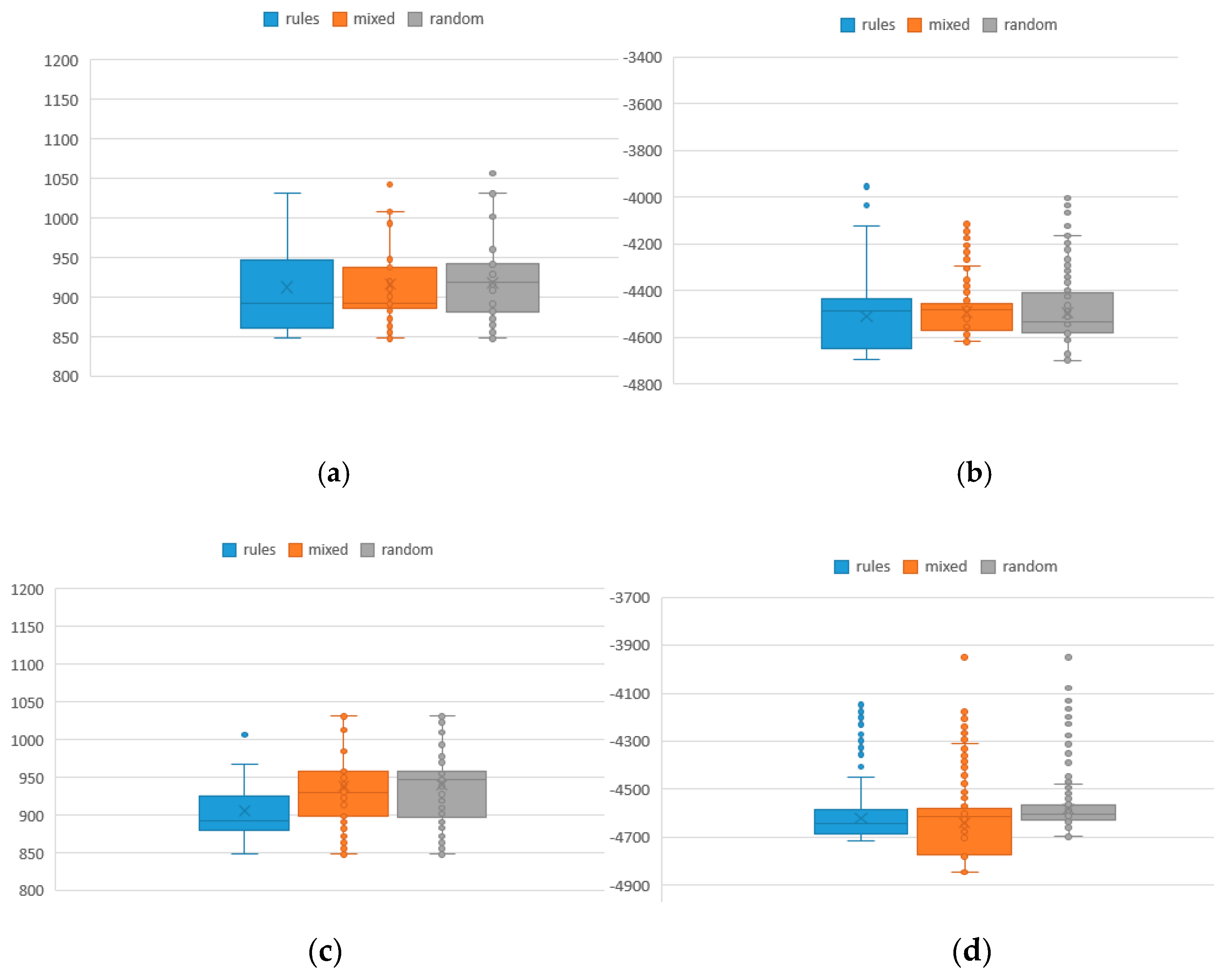
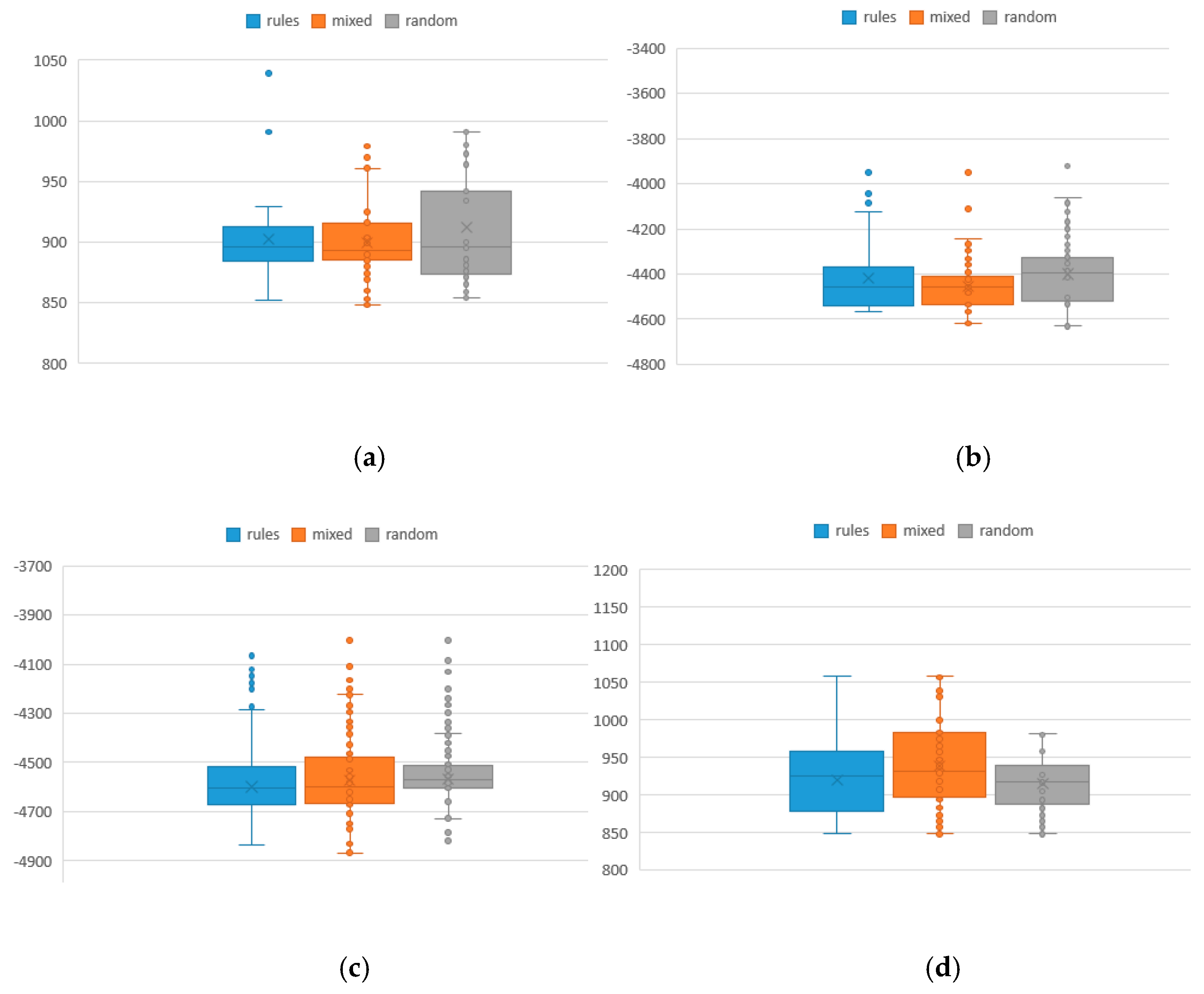
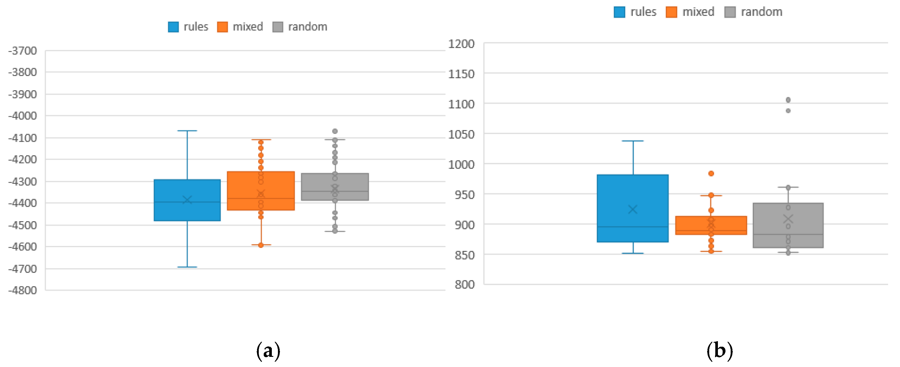
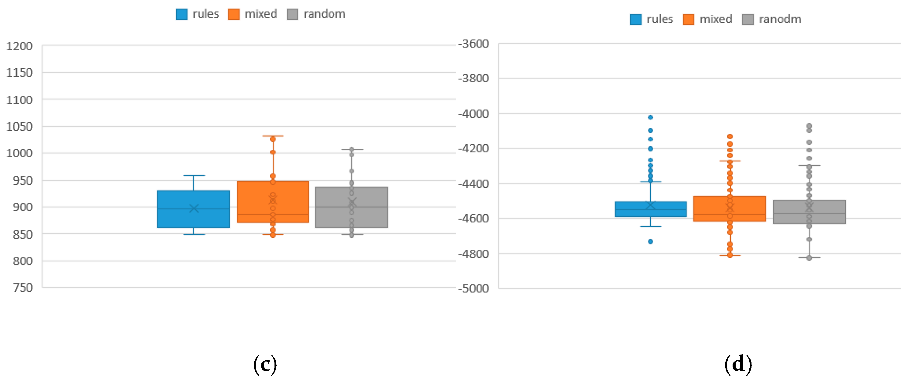
To analyze the values of the two objective functions and the average distribution from the optimal solution, the result of different iterations of 100 initial population is shown in

Table 9. Values of makespan, total tardiness, and RE of 100 initial population.

Methods	Iteration		F1	F2	RE
rules	100	best	848	−4696	7.5|4
		average	912	−4500	/
	300	best	848	−4717	6.7|2
		average	905	−4622	/
mixed	100	best	848	−4618	8.1|2.7
		average	916.3	−4492	/
	300	best	848	−4846	10.7|4.3
		average	939	−4639	/
random	100	best	848	−4698	8.4|4.3
		average	919	−4495	/
	300	best	848	−4698	11.2|2.4
		average	940	−4587	/

, where F1 and F2 represent the values of makespan and total tardiness, respectively, and the bold contents are better values. The rules method represents the new approach for population knowledge mining applied to the hybrid NSGA-II to solve MOJSSP. The traditional random method is the NSGA-II combined with SA for MOJSSP. The mixed method is a combination of the two methods. Figure 5 shows the box distribution of its function values of which the values in the rule method and the mixed method are overall smaller than the traditional method. To some extent, the smaller are the values, the better is the performance. Similarly, the results of different iterations of 50 and 25 initial population are shown in

Table 10. Values of makespan, total tardiness, and RE of 50 initial population.

Methods	Iteration		F1	F2	RE
rules	100	best	852	−4568	5.94|3.27
		average	902.6	−4418.4	/
	300	best	848	−4835	8.54|4.87
		average	920.4	−4599.3	/
mixed	100	best	848	−4618	6.03|3.52
		average	899.1	−4455.6	/
	300	best	848	−4868	10.74|6.04
		average	939.1	−4573.8	/
random	100	best	854	−4630	6.77|4.97
		average	911.8	−4400	/
	300	best	848	−4815	7.88|5.12
		average	914.8	−4568.5	/

and

Table 11. Values of makespan, total tardiness, and RE of 25 initial population.

Methods	Iteration		F1	F2	RE
rules	100	best	852	−4693	8.49|6.58
		average	924.3	−4384.3	/
	300	best	848	−4731	5.83|4.34
		average	897.4	−4525.9	/
mixed	100	best	855	−4593	5.38|5.11
		average	901	−4358.2	/
	300	best	848	−4810	7.63|5.59
		average	912.7	−4540.9	/
random	100	best	853	−4529	6.58|4.22
		average	909.1	−4337.8	/
	300	best	848	−4824	7.28|5.94
		average	909.7	−4537.4	/

. Figure 6 and Figure 7 are the box diagrams of the respective function values. From the results, we can find that the population mining method has more excellent results than the traditional random method because the rule population contains more excellent information than the traditional random population. Although the new method has no absolute advantage in the test of 25 initial population, it should be explained that, when the initial population size is too small, the performance of the method will inevitably be reduced. In general, there is no obvious advantage or disadvantage between rule method and mixed method in terms of function values, but, in term of the index RE, the rule method is superior to the mixed method, and both are superior to the random method. That is, the more rule-based individuals there are in the population, the more excellent information they contain, and thus it is easier to obtain excellent solutions under a limited number of iterations.

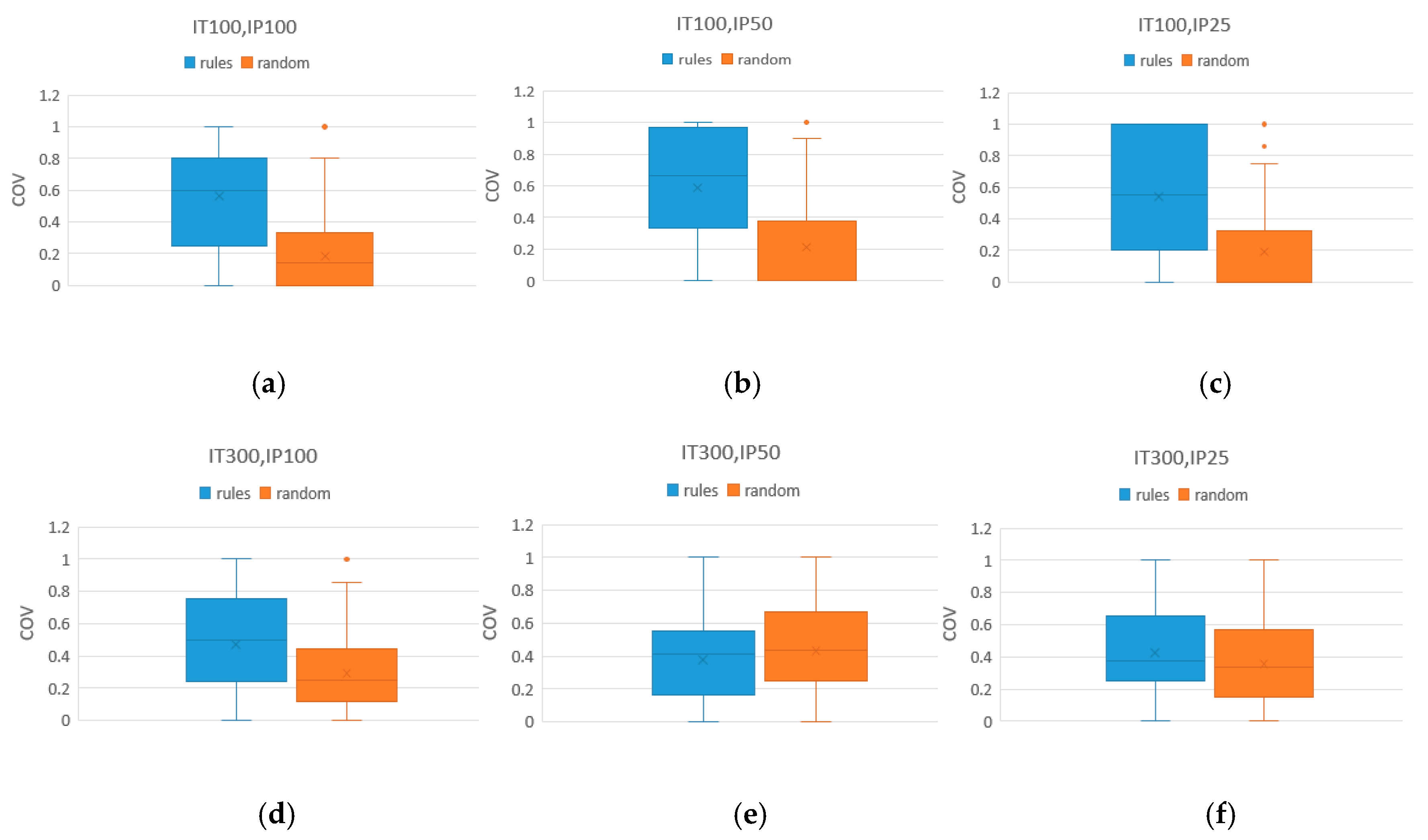
Since this paper optimizes two objectives at the same time, the values of makespan or total tardiness cannot be separately compared. Thus, the efficiency of the method was determined by the performance metrics of the acquired Pareto solutions, especially the dominance metric (Cov). Here, the performance metrics of the three methods are compared under different initial population sizes with the same number of iterations, as shown in

Table 12. Values of Cov and Spacing (rules vs. random).

Methods	IP		IT100		IT300
			Cov	Spacing	Cov	Spacing
rules	25	best	1	37	1	8.8
		average	0.54		0.4
	50	best	1	25	1	39
		average	0.59		0.38
	100	best	1	29	1	22
		average	0.56		0.47
random	25	best	0.75	76	1	50.5
		average	0.19		0.35
	50	best	0.9	65	1	45
		average	0.21		0.43
	100	best	0.8	37	0.86	18
		average	0.19		0.29

,

Table 13. Values of Cov and Spacing (mixed vs. random).

Methods	IP		IT100		IT300
			Cov	Spacing	Cov	Spacing
mixed	25	best	1	19	1	48
		average	0.63		0.31
	50	best	1	24	0.86	37
		average	0.45		0.35
	100	best	1	16	0.92	20
		average	0.41		0.45
random	25	best	0.27	76	1	50.5
		average	0.11		0.43
	50	best	1	65	1	45
		average	0.33		0.4
	100	best	1	37	1	18
		average	0.39		0.33

and

Table 14. Values of Cov and Spacing (rules vs. mixed).

Methods	IP		IT100		IT300
			Cov	Spacing	Cov	Spacing
rules	25	best	1	37	1	8.8
		average	0.24		0.46
	50	best	1	25	1	39
		average	0.47		0.44
	100	best	1	29	1	22
		average	0.53		0.41
mixed	25	best	1	19	0.8	48
		average	0.41		0.24
	50	best	1	24	0.88	37
		average	0.31		0.41
	100	best	1	16	1	20
		average	0.21		0.37

, where IP represents the size of the initial population and the bold contents are the better values. In Table 12, the Cov value of the rule method is generally higher than that of the traditional method. The larger is the Cov value, the higher is the dominant ability. That is, in terms of dominance, the rule method is superior to the traditional random method in comparing the size of different initial populations. At the same time, the Spacing values of the new method is generally smaller than that of the traditional method. From Equation (9), it can be seen that the distribution of the rule method is also superior to the random method in considering the initial population size as a variable. Figure 8 shows the box diagram of the Cov of the rule method vs. the random method. From the box diagram, we can find more intuitively that the Pareto solution of the rule method is superior to that of the traditional random method. Similarly, from the results in Table 13 and Table 14, we can conclude that the performance of rule method in Cov is also “rules > mixed > random”. For Spacing performance, the mixed method is better than the rule method, which shows that the mixed method can more easily obtain a uniformly distributed solution set with a limited number of iterations. Overall, the Spacing metrics of both the rule and mixed methods are superior to the random method.

To better illustrate the proposed ADSM, here we compare it with the Nasiri’s method. Compared with the operation sequence and knowledge constraints that are not considered,

Table 15. Comparison of function values of two rule-based populations.

Methods	IP	IT		F1	F2	RE
ADSM	25	100	best	852	−4693	8.49|6.58
			average	924.3	−4384.3	/
		300	best	848	−4731	5.83|4.34
			average	897.4	−4525.9	/
	50	100	best	852	−4568	5.94|3.27
			average	902.6	−4418.4	/
		300	best	848	−4835	8.54|4.87
			average	920.4	−4599.3	/
	100	100	best	848	−4696	7.5|4
			average	912	−4500	/
		300	best	848	−4717	6.7|2
			average	905	−4622	/
Nasiri’s	25	100	best	853	−4587	4|5.8
			average	887	−4319	/
		300	best	848	−4810	8.84|5.51
			average	923	−4545	/
	50	100	best	848	−4558	7.8|1.34
			average	914.2	−4497	/
		300	best	848	−4822	7.1|5.4
			average	908	−4561.5	/
	100	100	best	848	−4642	6|3.8
			average	896.3	−4467	/
		300	best	848	−4799	12.7|4.6
			average	956	−4576	/

shows that the proposed ADSM has an impact on the value of the single objective function. Although the advantage of the ADSM is not obvious in terms of single objective value, this is because the influence of local adjustment of operations on a single objective value is relatively small under multiple iterations. From the perspective of multi-objective, it significantly improves the performance metrics of dominance and distribution, as shown in

Table 16. Comparison of Cov and Spacing of two rule-based populations.

Methods	IP		IT100		IT300
			Cov	Spacing	Cov	Spacing
ADSM	25	best	1	37	1	8.8
		average	0.54		0.42
	50	best	1	25	1	39
		average	0.59		0.47
	100	best	1	29	1	22
		average	0.55		0.39
Nasiri’s	25	best	0.75	41	1	44
		average	0.19		0.35
	50	best	0.9	46	1	29
		average	0.21		0.33
	100	best	0.8	71	1	64
		average	0.16		0.37

. The results show that, under different iterations and initial population sizes, the Cov values and Spacing values of the ADSM are better, which demonstrates that it is more effective in solving multi-objective problems. On the other hand, the validity of the method ADSM is proved, which shows that the new proposed method can overcome the problem of sequencing the operations under knowledge mining as well as meet the requirement of high performance.

6. Conclusions

This paper presents a population knowledge mining approach combined with a hybrid machine learning algorithm to solve the MOJSSP with makespan and total tardiness criteria. The purpose of this method is to find a rule-based initial population from good production planning, which can produce better Pareto solutions than the traditional stochastic methods. Many optimal or near-optimal solutions are created by the method of NSGA-II integrated with SA on a benchmark of 10 × 10 job shop problem (LA18), and a training dataset with selected operations’ attributes is therefore acquired. For mining knowledge, the weight of priority is used to extract 37 potential rules, which map the relationship between the attribute set and priority.

To form the rule-based initial population, a complicated ADSM is proposed to assign each operation a priority class. This sorting method overcomes the problem of misalignment of the sequence of operations and overcomes the problem of insufficient or overflowing operations owned by the priority class. After generating an initial population set based on the data mining and ADSM, we compared it with the NSGA-II hybrid SA method of the mixed, random, and Nasiri’s initial population. Considering the different numbers of iterations and the sizes of the initial population, a series of comparative and computational experiments were conducted. The results show that the new proposed method is better than the traditional method in terms of the magnitude and relative error of each objective function, and the Cov and Spacing performance index of Pareto solutions.

The future works of our study will mainly focus on other methods of initial population formation and the application of the proposed method to other cases. Besides, considering other multi-objective problems and how to choose a mining algorithm to better improve the effect of rules need further research.

References

- Duan, Y.; Edwards, J.S.; Dwivedi, Y.K. Artificial intelligence for decision making in the era of Big Data–evolution, challenges and research agenda. Int. J. Inf. Manag. 2019, 48, 63–71. [Google Scholar] [CrossRef]
- Dai, H.; Wang, H.; Xu, G.; Wan, J.; Imran, M. Big data analytics for manufacturing internet of things: Opportunities, challenges and enabling technologies. Enterp. Inf. Syst. 2019, 1–25. [Google Scholar] [CrossRef] [Green Version]
- Kuo, Y.; Kusiak, A. From data to big data in production research: The past and future trends. Int. J. Prod. Res. 2019, 57, 4828–4853. [Google Scholar] [CrossRef] [Green Version]
- Lin, S.; Dong, C.; Chen, M.; Zhang, F.; Chen, J. Summary of new group intelligent optimization algorithms. Comput. Eng. Appl. 2018, 54, 1–9. [Google Scholar]
- Gao, L.; Pan, Q. A shuffled multi-swarm micro-migrating birds optimizer for a multi-resource-constrained flexible job shop scheduling problem. Inf. Sci. 2016, 372, 655–676. [Google Scholar] [CrossRef]
- Ruiz, R.; Pan, Q.; Naderi, B. Iterated Greedy methods for the distributed permutation flowshop scheduling problem. Omega 2019, 83, 213–222. [Google Scholar] [CrossRef]
- Dao, T.; Pan, T.; Nguyen, T.; Pan, J. Parallel bat algorithm for optimizing makespan in job shop scheduling problems. J. Intell. Manuf. 2018, 29, 451–462. [Google Scholar] [CrossRef]
- Fan, B.; Yang, W.; Zhang, Z. Solving the two-stage hybrid flow shop scheduling problem based on mutant firefly algorithm. J. Ambient Intell. Humaniz. Comput. 2019, 10, 979–990. [Google Scholar] [CrossRef]
- Li, M.; Lei, D.; Cai, J. Two-level imperialist competitive algorithm for energy-efficient hybrid flow shop scheduling problem with relative importance of objectives. Swarm Evol. Comput. 2019, 49, 34–43. [Google Scholar] [CrossRef]
- Gong, G.; Deng, Q.; Chiong, R.; Gong, X.; Huang, H. An effective memetic algorithm for multi-objective job-shop scheduling. Knowl. Based Syst. 2019, 182, 104840. [Google Scholar] [CrossRef]
- Wiemer, H.; Drowatzky, L.; Ihlenfeldt, S. Data mining methodology for engineering applications (DMME)—A holistic extension to the CRISP-DM model. Appl. Sci. 2019, 9, 2407. [Google Scholar] [CrossRef] [Green Version]
- Koonce, D.A.; Tsai, S.C. Using data mining to find patterns in genetic algorithm solutions to a job shop schedule. Comput. Ind. Eng. 2000, 38, 361–374. [Google Scholar] [CrossRef]
- Wu, B.; Hao, K.; Cai, X.; Wang, T. An integrated algorithm for multi-agent fault-tolerant scheduling based on MOEA. Future Gener. Comput. Syst. 2019, 94, 51–61. [Google Scholar] [CrossRef]
- Huang, X. A hybrid genetic algorithm for multi-objective flexible job shop scheduling problem considering transportation time. Int. J. Intell. Comput. Cybern. 2019, 12, 154–174. [Google Scholar] [CrossRef]
- Souier, M.; Dahane, M.; Maliki, F. An NSGA-II-based multiobjective approach for real-time routing selection in a flexible manufacturing system under uncertainty and reliability constraints. Int. J. Adv. Manuf. Technol. 2019, 100, 2813–2829. [Google Scholar] [CrossRef]
- Ahmadi, E.; Zandieh, M.; Farrokh, M.; Emami, S.M. A multi objective optimization approach for flexible job shop scheduling problem under random machine breakdown by evolutionary algorithms. Comput. Oper. Res. 2016, 73, 56–66. [Google Scholar] [CrossRef]
- Zhou, Y.; Yang, J.; Zheng, L. Hyper-heuristic coevolution of machine assignment and job sequencing rules for multi-objective dynamic flexible job shop scheduling. IEEE Access 2019, 7, 68–88. [Google Scholar] [CrossRef]
- Zhang, R.; Chiong, R. Solving the energy-efficient job shop scheduling problem: A multi-objective genetic algorithm with enhanced local search for minimizing the total weighted tardiness and total energy consumption. J. Clean. Prod. 2016, 112, 3361–3375. [Google Scholar] [CrossRef]
- Du, W.; Zhong, W.; Tang, Y.; Du, W.; Jin, Y. High-dimensional robust multi-objective optimization for order scheduling: A decision variable classification approach. IEEE Trans. Ind. Inform. 2019, 15, 293–304. [Google Scholar] [CrossRef] [Green Version]
- Sheikhalishahi, M.; Eskandari, N.; Mashayekhi, A.; Azadeh, A. Multi-objective open shop scheduling by considering human error and preventive maintenance. Appl. Math. Model. 2019, 67, 573–587. [Google Scholar] [CrossRef]
- Lu, C.; Gao, L.; Pan, Q.; Li, X.; Zheng, J. A multi-objective cellular grey wolf optimizer for hybrid flowshop scheduling problem considering noise pollution. Appl. Soft Comput. 2019, 75, 728–749. [Google Scholar] [CrossRef]
- Qin, H.; Fan, P.; Tang, H.; Huang, P.; Fang, B.; Pan, S. An effective hybrid discrete grey wolf optimizer for the casting production scheduling problem with multi-objective and multi-constraint. Comput. Ind. Eng. 2019, 128, 458–476. [Google Scholar] [CrossRef]
- Zhou, Y.; Yang, J.; Zheng, L. Multi-agent based hyper-heuristics for multi-objective flexible job shop scheduling: A case study in an aero-engine blade manufacturing plant. IEEE Access 2019, 7, 21147–21176. [Google Scholar] [CrossRef]
- Fu, Y.; Wang, H.; Huang, M. Integrated scheduling for a distributed manufacturing system: A stochastic multi-objective model. Enterp. Inf. Syst. 2019, 13, 557–573. [Google Scholar] [CrossRef]
- Ingimundardottir, H.; Runarsson, T.P. Discovering dispatching rules from data using imitation learning: A case study for the job-shop problem. J. Sched. 2018, 21, 413–428. [Google Scholar] [CrossRef]
- Li, X.; Olafsson, S. Discovering dispatching rules using data mining. J. Sched. 2005, 8, 515–527. [Google Scholar] [CrossRef]
- Olafsson, S.; Li, X. Learning effective new single machine dispatching rules from optimal scheduling data. Int. J. Prod. Econ. 2010, 128, 118–126. [Google Scholar] [CrossRef]
- Jun, S.; Lee, S.; Chun, H. Learning dispatching rules using random forest in flexible job shop scheduling problems. Int. J. Prod. Res. 2019, 3290–3310. [Google Scholar] [CrossRef]
- Kumar, S.; Rao, C.S.P. Application of ant colony, genetic algorithm and data mining-based techniques for scheduling. Robot. Comput. Integr. Manuf. 2009, 25, 901–908. [Google Scholar] [CrossRef]
- Nasiri, M.M.; Salesi, S.; Rahbari, A.; Salmanzadeh Meydani, N.; Abdollai, M. A data mining approach for population-based methods to solve the JSSP. Soft Comput. 2019, 23, 11107–11122. [Google Scholar] [CrossRef]
- Hillier, F.S.; Lieberman, G.J. Introduction to Operations Research, 7th ed.; McGraw-Hill Science: New York, NY, USA, 2001. [Google Scholar]
- Lawrence, S. An Experimental Investigation of Heuristic Scheduling Techniques; Carnegie-Mellon University: Pittsburgh, PA, USA, 1984. [Google Scholar]
- Fu, Y.; Wang, H.; Tian, G.; Li, Z.; Hu, H. Two-agent stochastic flow shop deteriorating scheduling via a hybrid multi-objective evolutionary algorithm. J. Intell. Manuf. 2019, 30, 2257–2272. [Google Scholar] [CrossRef]
- Cai, Y. Attribute-Oriented Induction in Relational Databases, Knowledge Discovery in Databases. Ph.D. Thesis, Simon Fraser University, Burnaby, BC, Canada, 1989. [Google Scholar]
- González-Briones, A.; Prieto, J.; De La Prieta, F.; Herrera-Viedma, E.; Corchado, J. Energy optimization using a case-based reasoning strategy. Sensors 2018, 18, 865. [Google Scholar] [CrossRef] [Green Version]
- Deb, K.; Pratap, A.; Agarwal, S.; Meyarivan, T. A fast and elitist multiobjective genetic algorithm: NSGA-II. IEEE Trans. Evol. Comput. 2002, 2, 182–197. [Google Scholar] [CrossRef] [Green Version]
- Kirkpatrick, S.; Gelatt, C.D.; Vecchi, M.P. Optimization by simulated annealing. Science 1983, 4598, 671–680. [Google Scholar] [CrossRef] [PubMed]
- Cobos, C.; Erazo, C.; Luna, J.; Mendoza, M.; Gaviria, C.; Arteaga, C.; Paz, A. Multi-objective memetic algorithm based on NSGA-II and simulated annealing for calibrating CORSIM micro-simulation models of vehicular traffic flow. In Conference of the Spanish Association for Artificial Intelligence; Springer: Cham, Switzerland, 2016. [Google Scholar]
- Zitzler, E.; Thiele, L. Multiobjective evolutionary algorithms: A comparative case study and the strength pareto approach. IEEE Trans. Evol. Comput. 1999, 3, 257–271. [Google Scholar] [CrossRef] [Green Version]
- Schott, J.R. Fault Tolerant Design Using Single and Multicriteria Genetic Algorithm Optimization; Massachusetts Institute of Technology: Cambridge, MA, USA, 1995. [Google Scholar]
- Arroyo, J.E.C.; Leung, J.Y.T. An effective iterated greedy algorithm for scheduling unrelated parallel batch machines with non-identical capacities and unequal ready times. Comput. Ind. Eng. 2017, 105, 84–100. [Google Scholar] [CrossRef]
Figure 1.
Process of the proposed approach for MOJSSP.
Figure 2.
Processing time attribute.
Figure 3.
Remaining time attribute.
Figure 4.
Framework of ADSM.
Figure 5.
Distribution of makespan and total tardiness of 100 initial population sizes under different iteration numbers: (a) makespan under 100 iterations; (b) total tardiness under 100 iterations; (c) makespan under 300 iterations; and (d) total tardiness under 300 iterations.
Figure 6.
Distribution of makespan and total tardiness of 50 initial population sizes under different iteration numbers: (a) makespan under 100 iterations; (b) total tardiness under 100 iterations; (c) makespan under 300 iterations; and (d) total tardiness under 300 iterations.
Figure 7.
Distribution of makespan and total tardiness of 25 initial population sizes under different iteration numbers: (a) makespan under 100 iterations; (b) total tardiness under 100 iterations; (c) makespan under 300 iterations; and (d) total tardiness under 300 iterations.
Figure 8.
Box diagram of Cov of the rule method vs. random method with different sizes of initial population under 100 and 300 iterations: (a) IP = 25 under 100 iterations; (b) IP = 50 under 100 iterations; (c) IP = 100 under 100 iterations; (d) IP = 25 under 300 iterations; (e) IP = 50 under 300 iterations; and (f) IP = 100 under 300 iterations.