Predicting the Extreme Loads in Power Production of Large Wind Turbines Using an Improved PSO Algorithm

1
Institute of Engineering Thermophysics, Chinese Academy of Sciences, Beijing 100190, China
2
Key Laboratory of Wind Energy Utilization, Chinese Academy of Sciences, Beijing 100190, China
3
National Research and Development Center of Wind Turbine Blade, Beijing 100190, China
*
Author to whom correspondence should be addressed.
Appl. Sci. 2019, 9(3), 521; https://doi.org/10.3390/app9030521
Submission received: 24 December 2018
/
Revised: 23 January 2019
/
Accepted: 31 January 2019
/
Published: 3 February 2019
(This article belongs to the Special Issue Wind Energy Conversion Systems)
Abstract
:Predicting the extreme loads in power production for the preliminary-design of large-scale wind turbine blade is both important and time consuming. In this paper, a simplified method, called Particle Swarm Optimization-Extreme Load Prediction Model (PSO-ELPM), is developed to quickly assess the extreme loads. This method considers the extreme loads solution as an optimal problem. The rotor speed, wind speed, pitch angle, yaw angle, and azimuth angle are selected as design variables. The constraint conditions are obtained by considering the influence of the aeroelastic property and control system of the wind turbine. An improved PSO algorithm is applied. A 1.5 MW and a 2.0 MW wind turbine are chosen to validate the method. The results show that the extreme root load errors between PSO-ELPM and FOCUS are less than 10%, while PSO-ELPM needs much less computational cost than FOCUS. The distribution of flapwise bending moments are close to the results of FOCUS. By analyzing the loads, we find that the extreme flapwise bending moment of the blade root in chord coordinate (CMF_ROOT) is largely reduced because of the control system, with the extreme edgewise bending moment of the blade root in chord coordinate (CME_ROOT) almost unchanged. Furthermore, higher rotor speed and smaller pitch angle will generate larger extreme bending moments at the blade root.
1. Introduction
With the increased utilization of low wind speed, blade lengths are becoming increasingly longer, so as to capture more energy at low wind speed. By contrast, in order to control costs, the other parts of the wind turbine have largely remained the same. In fact, this treatment implies that the extreme loads, especially the extreme loads at the blade root are constant or increase within the accepted margin of safety during blade design. Therefore, the extreme load at the blade root is one of the most important constraints when designing of low wind speed blades and blade bolts, even though the blade can reliably endure the loads acting on itself. Of course, the extreme load distribution is also critical factor in the evaluation of the safety of blade. However, in this paper we focus on the extreme load prediction at the blade root because it can be easily extended to get the extreme load distribution.
As far as we know, calculating the extreme loads according to the IEC [1] or GL [2] standard is extremely time consuming. Over the last decade, most researchers extrapolated the extreme loads by means of statistical methods which suppose that the distribution of extreme loads at different wind speed meet some statistical models [3,4,5,6,7,8,9,10,11,12,13,14,15]. Generally, it is reasonable to estimate the extreme loads that occur or a long duration based on the measured or simulated data gathered over a short period. However, these methods are not without their drawbacks. These issues include, which distribution method should be used for the estimation of the short-term extreme load distribution? What are the criteria for the selection of the maximum loads used in the extreme load distribution? And how many time series, simulated or measured, are needed for the proper estimated of the extreme load distribution? [4] Naturally, more data gives better results, however by increasing the number of simulated load cases, the time taken to conduct these simulations is drastically increased. During the design of the blade, the discrete engineering method, has been widely adopted to obtain accurate results. This method gives the extreme loads by simulating every load case according to the IEC or GL standard. Most software programs, such as PHATAS in FOCUS [16] and Bladed [17], all employ this method. This method is more accurate than statistical methods. But the process of this method is also time-consuming and unsuitable for the preliminary design due to excessive load cases required to be simulated during the design life of the wind turbine. For simplicity, many research articles about the design methods regarding blade optimization design select parts of the design load cases (DLCs) to get the extreme load and finally run all the DLCs to verify the results to reduce the overall computational time [18,19,20,21,22]. Even though this process has been used to save time, it takes about 65 h running on a workstation equipped with 40 logical processors [20]. Therefore, this process still represents low efficiency, and it is therefore necessary to propose a new method that can quickly predict the extreme loads for the preliminary design of large-scale wind turbine blades.
In this paper, a simplified method is proposed to quickly predict the extreme loads in power production to facilitate the preliminary design of the blades. The optimal algorithm is used to acquire the extreme loads. Because the blade loads are affected by a number of factors, the solution of predicting extreme loads is a combination of multi-variable, multi-constraint, and multi-object optimal problem. An advanced intelligent optimal algorithm should be found to solve this kind of constraint optimal problem. Compared with the genetic algorithm (GA), the PSO algorithm has its own advantages, such as a simpler and less adjusting parameters. Hence, a simplified extreme load prediction model (PSO-ELPM) by use of an improved PSO algorithm [5] is built and certified by comparing with the results from FOCUS using the discrete method. The results show that the extreme root load errors between PSO-ELPM and FOCUS are less than 10%, while PSO-ELPM needs much less computational cost than FOCUS. The distribution of flapwise bending moments are close to the results of FOCUS. In addition, PSO-ELPM can directly get the status parameters generating extreme loads. This will be useful for control rules design of wind turbines.
2. Model Building
To establish the optimal model for predicting extreme forces, the free variables, constraints, and fitness function need be determined. As we know, the blade loads, especially the flapwise loads, are mainly generated by aerodynamic force. Therefore, the parameters in the equation of aerodynamic force will be mainly analyzed and selected as free variables. Furthermore, the level of gravity is also critical for the edgewise force and will be considered in the solution of fitness function.
In reality, the extreme loads always produce a certain status with few features. According to the IEC and GL standard, the extreme DLCs always selected the rated wind speed , and to do the simulation. This is because the extreme loads are always generated around the rated wind speed. However, in this case, the rotor speed always reaches the max value, and the pitch angle usually approximates the minimum value. Therefore, the ability to find the minimum pitch angle and corresponding rotor speed is very important. However, if we calculate the blade load using the dynamic aeroelastic simulation, it will increase the amount of unnecessary calculations because many of the statuses will not generate the extreme value. Therefore, in order to reduce the computational time, a quasi-static load computation with a considerstion of the status parameters of the wind turbine is used in this article. Certainly, storm conditions can be the worst conditions due to large wind speed and inflow angle. Such conditions are not considered in this model, but will be added in the future.
2.1. Design Variables
The corresponding parameters in the aerodynamic force as the main source of the blade load will be selected as the design variables. The aerodynamic force acting on a blade section under the wind speed is shown as Figure 1. The normal force and the tangential force could be expressed as follows:
where ρ is the air density, c is chord length, , are respectively the normal coefficient and tangential coefficient as:
where is the lift coefficient, is the drag coefficient, ϕ is the inflow angle, from which the attack angle α will be get by subtracting the twist angle and pitch angle , i.e.,
The inflow velocity in Equation (1) is
where a is the axial induction factor, b is the tangential induction factor, is angular speed of the rotor shaft, that is rotor speed in this article.
It can be seen that the load is influenced by lots of variables from Equation (1), such as the wind speed, the chord length, and the pitch angle. Moreover, the wind turbine parameters such as yaw angle γ, azimuth angle ψ also affect the angle between the wind direction and chord line, so they are all taken into account to obtain the extreme loads. However, some of them are prefixed. Therefore, the rotor speed, wind speed, pitch angle, yaw angle, and azimuth angle will be selected as design variables.
2.2. Design Constraints
After the aerodynamic profile and structure of the blade are fixed, the blade load chiefly depends on rotor speed, pitch angle, and wind speed. However, the above parameters are not independent due to the operation of the control system. Their relationships are nonlinear and changing with the initial condition and time. It is therefore hard to get the specific relationships from them. For the optimal problem, we only need the bound values of these variables and the constraint conditions of the bound values.
2.2.1. Constraints on Pitch Angle
In the following analysis, a 1.5 MW variable speed and variable pitch (VSVP) wind turbine is taken as an example. The constraint conditions will be built by analyzing different load cases, which are simulated with a consideration of the aeroelastic property and the action of the control system by using PHATAS model in FOCUS software.
Constraints between Pitch Angle and Wind Speed
The minimum pitch angle for the wind speed is expressed by . For VSVP wind turbine, the blade pitch angle will get larger with the increase of the wind speed so as to reduce the rotor speed. Various pitch angles may occur while the wind turbine operates at the same wind speed due to the control system. Hence, obtaining the minimum pitch angle for a wind speed is very difficult, and also the key point of data that is requires so as to confirm the accuracy of the PSO-ELPM.
A variety of load cases have been computed in compliance with GL standard [20], especially the load cases that make it easy to generate the extreme loads, such as the DLC 1.6 and DLC 4.2. Figure 2 gives the different pitch angles for different wind speeds during the simulation of DLC 1.X (X expressed by the number 3, 4, 5, 6, 7, 8, 9) and DLC 4.2, which are computed by FOCUS.
From Figure 2, we can see that the varies with wind speeds. When the wind speed is less than 15 m/s, can reach the installation angle. But when the wind speed is above 15 m/s, becomes larger and larger with the increase of wind speed. Practically, will also change with the variation of the aerodynamic profile, blade layers and control strategy at the same wind speed. In this paper, a rough and versatile method is used to get . Because the extreme DLCs simulate the extreme condition suddenly occurring during the normal operation of wind turbine, the variation of the pitch angle will be not far away from the steady condition by using control system and safety system. Therefore, the is set as the maximum offset value away from the pitch angle under the condition of steady operation. That is to say, if the pitch angle is 10 degrees when the wind turbine normally operates at 15 m/s, the minimum pitch angle is equal to 10 − Δβ2 at 15 m/s for all load cases. Practically, may be different for different wind speeds. In order to simplify it, is set as a constant. The can be obtained from the calculation results of all load cases or part of the load cases. For this 1.5 MW wind turbine, is 10.86 degree from part of the load cases computed by FOCUS.
Considering the limitation of the installation angle , the for different wind speeds is shown with red triangles in Figure 2. Based on Figure 2, the versus wind speed V1 is divided into three sections.
For the first section, is equal to when the wind speed is less than , which is always the rated wind speed. So, it can be expressed as:
For the second section, is deduced by the offset from the steady operation value when is between and Vout. For VSVP wind turbine, the steady curve can be expressed as:
where B1, B2, and B3 are constant and can be obtained by quadratic polynomial fitting. Data for fitting, which are assessed by simulating the steady operation of the wind turbine using FOCUS, are expressed as green circle in Figure 2.
Therefore, βv can be expressed as:
Besides, βv cannot be less than βl, so
For the third section, V1 is larger than Vo. Under this condition, the wind turbine exceeds the normal operational range. The safety system will work and make the pitch angle change to feather. It will not stop until the pitch angle reaches the allowed maximum value, which is around 90 degrees. So the relationship of versus V1 is assumed as a straight line, which is through the point (Vo, βo) with the slope of pitch rate Kp, from Vo to the maximum wind speed. Then, the βv can be expressed as:
The point (Vo, βo) also matches Equation (8) to guarantee the continuity of the value of βv. That is,
Constraints between Pitch Angle and Rotor Speed
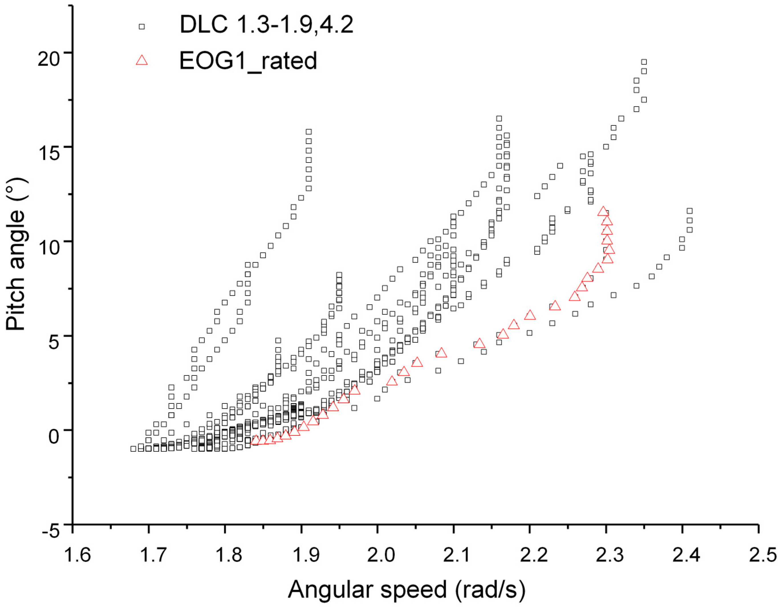
The minimum pitch angle for rotor speed is expressed by βr. Figure 3 depicts the different pitch angles for different rotor speeds during the simulation of DLC 1.X (X expressed by the number 3, 4, 5, 6, 7, 8, 9) and DLC 4.2. EOG1_Rated means that the data are obtained from the simulation of an extreme load case, which of the inflow condition is an extreme operational gust in one year (EOG1) at rated wind speed. From Figure 3, it is clear that the βr has different values for different rotor speeds. When the rotor speed is less than 1.82 rad/s, βr can reach the installation angle. But when the rotor speed is above 1.82 rad/s, βr increases with the rotor rise of speed.
However, it is very complicated to accurately attain βr. Based on Figure 3, the βr versus wind speed V1 is divided into two sections. For the first section, βr equal to βr when the rotor speed is less than Ω′, which is always the rated rotor speed Ωr. It can be expressed as:
For the second section, βr approaches a straight line when the rotor speed is above Ω′ and it can be expressed as
where C1 and C2 are the constant and can be obtained from a linear fitting, based on the data shown in the red triangle in Figure 3. These data are obtained by simulating load case with inflow conditions satisfied by EOG1 at rated wind speed, using FOCUS. It also can be experientially given.
Certainly, βr cannot be less than βl, so
Brief Summary
According to the above analysis, we can get the minimum pitch angle for a given rotor speed and wind speed, named as βm, can be defined as
Therefore, for all the rotor speeds and wind speeds, the corresponding pitch angle should not be lower than βm, that is
In addition, the pitch angle should be below the allowed maximum value βu, which is around 90 degrees. Therefore, the pitch angle should satisfy the following inequality constraint.
2.2.2. Other Constraints
For VSVP wind turbine, there is always a maximum rotor speed Ωb, where the safety system will work to limit the rotor speed. Certainly, because of the delay of the actuator, the rotor speed still has a certain incremental value ΔΩ. However, it is difficult to fix. According to the known results from the simulation of FOCUS, it is no more than 0.2 times the rated rotor speed. Therefore, the rotor speed may get the maximum value as
In this article, we used the maximum rotor speed appeared in FOCUS analysis. In Section 3, we will discuss the effects of parameter ΔΩ on the extreme load.
Moreover, the range of the other variables should be confined in compliance with the wind farm class and the design requirements of the wind turbine.
2.2.3. Summary of Constraints
According to the above analysis, Equations (18) and (20) are finally used to limit the change of the design variables. In order to get the βm in Equation (18), Equations (6), (8)–(16) are needed, we can see that there are many parameters that need to be fixed in these equations. Fortunately, some of the parameters in the above equations are given before can begin the blade design. They are βu, βl, Kp, Ωl, Ωb, Vl, Vu, γl, γu, ψl, ψu. How to get the unknown parameters except ΔΩ is given below in detail.
Step 1: We conduct the steady simulation to get the rotor speed, pitch angle, and output power changing with time.
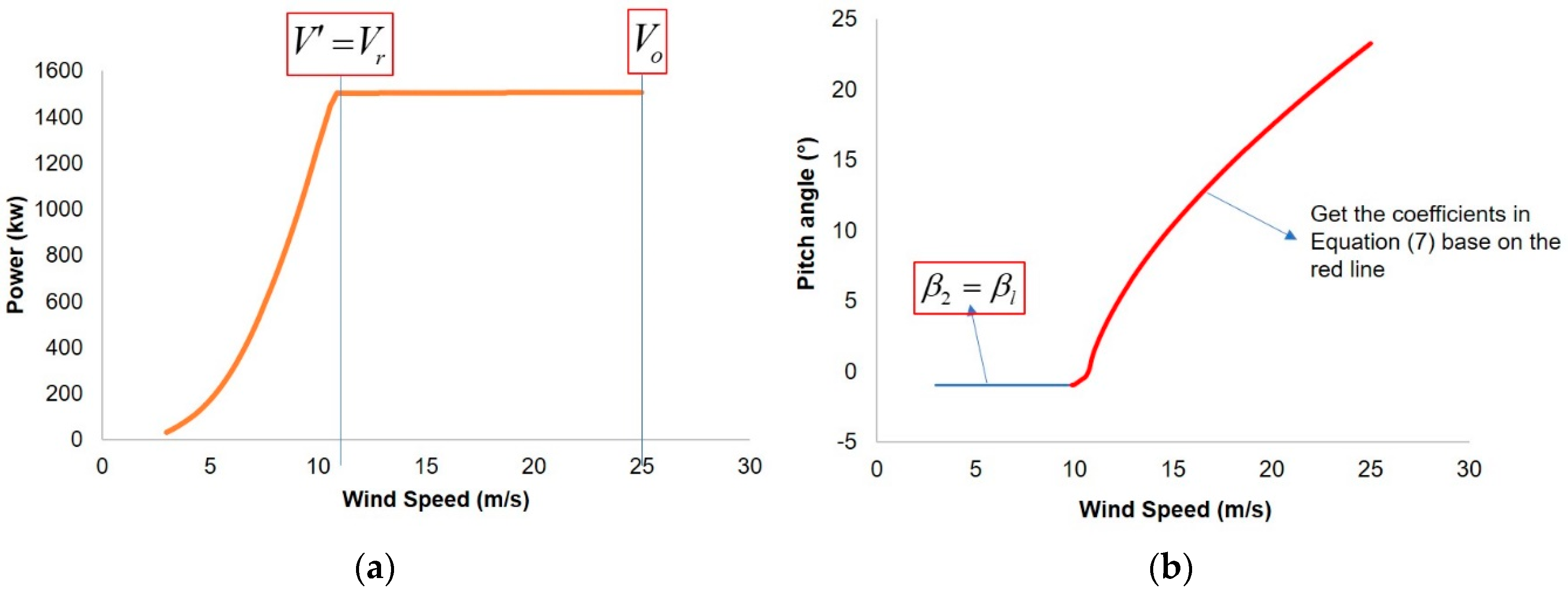
Step 2: According to the steady simulation, some parameters can be obtained, such as Vr, Ωr, and Vo. Following this, V′ is obtained from power versus wind speed (see (a) in Figure 4).
Step 3: Based on the pitch angle changing with wind speed, we can get the coefficients in Equation (7) by quadratic polynomial fitting (see (b) in Figure 4).
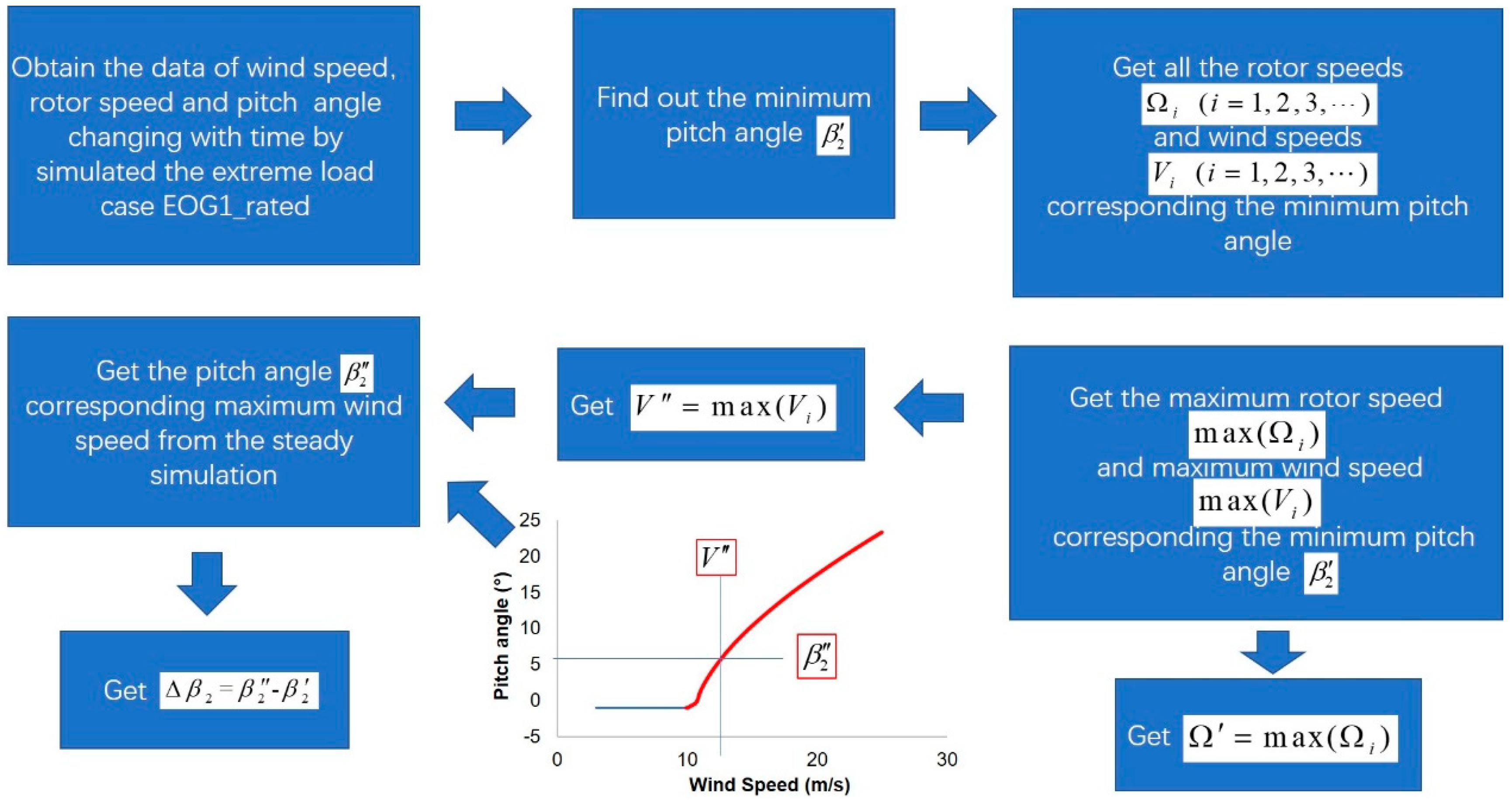
Step 4: By computing the extreme load case with the inflow wind condition, which is satisfied EOG1 at rated wind speed, using FOCUS, we can obtain the data in Figure 2 and Figure 3. Then Δβ2 and Ω′ can be obtained using the following method (see Figure 5).
Step 5: We can get the parameter βo according to Equation (11).
Step 6: From the simulation results in step 4 (see the red triangles in Figure 3), we can access the coefficients in Equation (13) by linear fitting.
2.3. Design Objects
For the large-scale blade used in the low wind speed area, the extreme load, especially the extreme bending moment at the blade root plays a key role in the blade design. It not only influences the blade reliability, but also involves the security of other equipment, such as the pitch motor and connecting bolts. Hence, for the single objective optimization, the extreme moment in one direction at a given section is selected as the design object. For the multi-objective optimization, the design objects can be defined as the different direction bending moments at the same section, or the same direction bending moment at different sections, or the different direction bending moments at different sections.
To compute the bending moments at different sections, the blade element moment (BEM) theory is chosen to obtain the aerodynamic force Fa, which are Fn and Ft in Equation (1). From Equations (1)–(5), we can see that the induction factors of a and b are the only unknown numbers, while the other parameters are known or the design variables. In this article, the traditional iteration algorithm for BEM is used to obtain them with considering the tip loss correction and root loss correction. It is as follows.
Step 1: Supposing initial values for a and b, such as a = 0, b = 0;
Step 2: Using Equation (4) to get the inflow angle;
Step 3: Using Equation (3) to get the attack angle;
Step 4: Computing the blade loss factor F = FtipFhub;
Where Ftip is tip loss factor, Fhub is root loss factor. They are shown as
where B is the number of the blade, R is the rotating radius of rotor, Rhub is the rotating radius of hub, r is the rotating radius of blade element.
Step 5: Computing the thrust coefficient of the rotor CT;
where σ is rotor solidity and it is shown as
Step 6: If , the new induction factor a′ will be computed by Equation (25);
where , , or else, the new induction factor a′ will be computed by Equation (26).
Step 7: The new induction factor b′ will be computed by Equation (27);
Step 8: Computing the error and ;
Step 9: If and , end the iteration and use a′, b′ and Equations (1)–(5) to get the Fn and Ft, that is Fa or else, return to step 2 use new induction factor a′ and b′.
Moreover, the gravity Fg and centrifugal force Fc at different section is also taken into account. They are shown as follows
where is section mass per length, g is gravity acceleration.
Then, we can obtain the force Fk at a certain section by coordinate transformation.
Supposing that Fk is not changing along one blade element, the forces and moments at a section in a certain coordinate can be solved by coordinate transformation and integration.
Finally, the flow chart of the blade load calculation model is given below (see Figure 6).
2.4. Building the PSO-ELPM Model
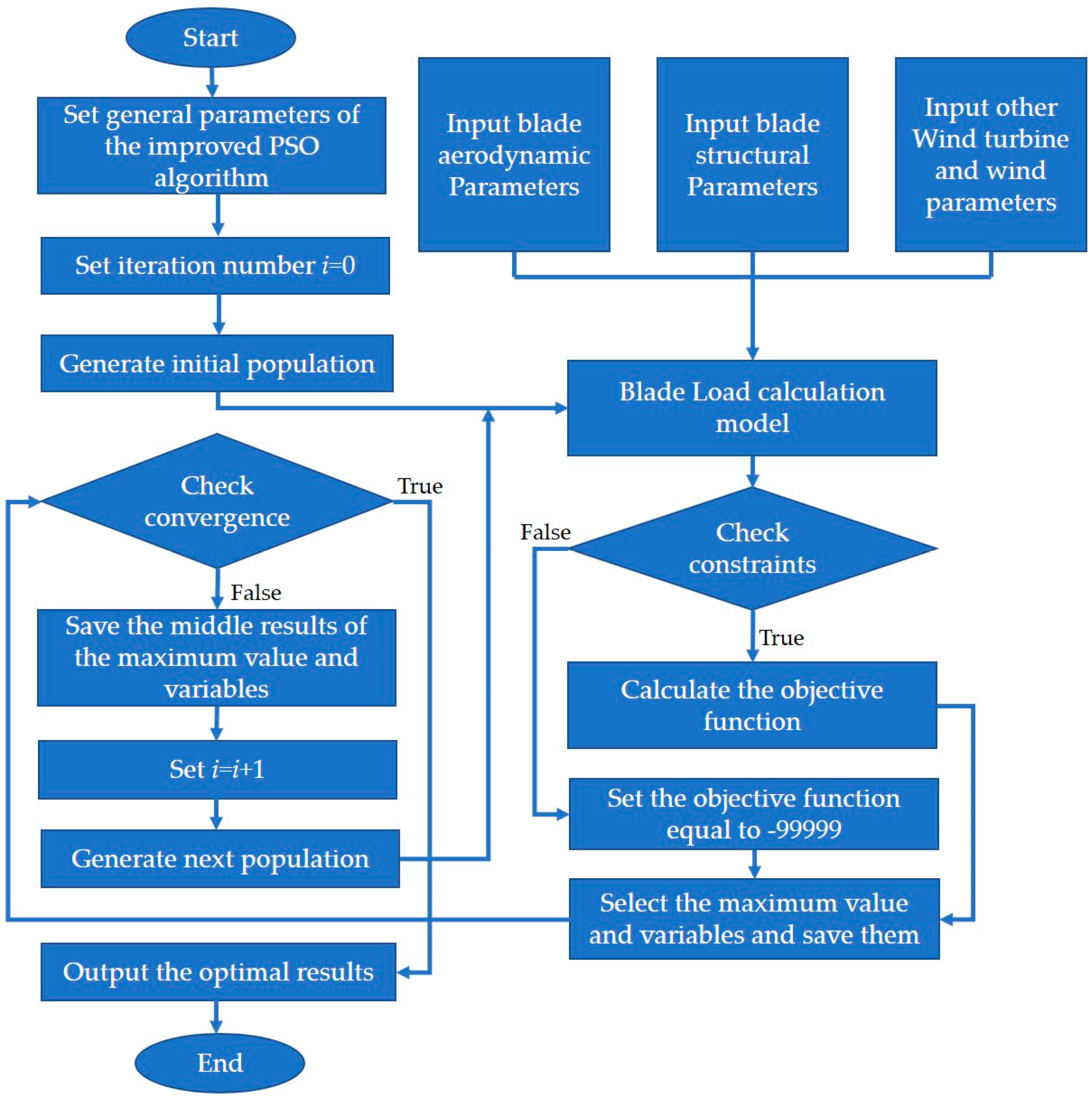
In this article, an improved PSO algorithm [5] developed by the authors is employed to evaluate the extreme loads. This optimal algorithm has a better optimization capability than the original PSO algorithm. It is suitable for multi-variables, discontinuous, and multi-objects problem. Finally, by combining the blade load calculation model and the improved PSO algorithm, a simplified extreme load predicting model (PSO-ELPM) is built. The flow chart of PSO-ELPM is given below (see Figure 7).
3. Results and Discussion
The model proposed in the paper was applied to a 1.5 MW VSVP wind turbine and a 2.0 MW VSVP wind turbine to predict the bending moments at the blade root. The corresponding results were compared with those computed by FOCUS [12] to validate the model. The particular constraint conditions used in the PSO-ELPM is introduced firstly.
- (1)
- For the 1.5 MW VSVP wind turbine, the constraint conditions werewhere βv satisfies the following expressions.and βr satisfies the following expressions.The other variables satisfy the following inequalities.
- (2)
- For the 2.0 MW VSVP wind turbine, the constraint conditions werewhere βv can be formulated as:and βr is:The other variables can be defined as:
Then, in order to compare with the results from FOCUS, the load factor γF will be considered. According to the GL standard, γF is set to be 1.35.
Moreover, the related parameters in the improved PSO algorithm are prefixed as follows:
- (1)
- Number of individuals: 30;
- (2)
- Maximum number of iterations: 100;
- (3)
- Probability of selection Ps: 0.0333;
- (4)
- Maximum inertial weight: 0.6253;
- (5)
- Minimum inertial weight: 0.0562
3.1. Extreme Loads at the Blade Root
Finally, the maximum flapwise bending moment of blade root in chord coordinate (CMF_ROOT) and the maximum edgewise bending moment of blade root in chord coordinate (CME_ROOT) was calculated respectively by the PSO-ELPM model. Each of them was computed ten times independently. Figure 8 and Figure 9 give the iterative processes, from which the extreme CMF_ROOT and the extreme CME_ROOT was obtained. The extreme values of CMF_ROOT and CME_ROOT are shown in Table 1. The status parameters of the wind turbine, while the extreme loads were reached, are given to highlight in Table 2.
From Table 1, it can be seen that the results using PSO-ELPM are well in agreement with those using FOCUS, with a difference of less than 10%. Especially for the extreme CMF_ROOT, the error was lower than 5%. It shows that PSO-ELPM can be used for predicting the extreme load. Moreover, PSO-ELPM needs much less computational cost than FOCUS. That is, PSO-ELPM only needs about 50 min to get the extreme CMF_ROOT (ten times calculation) while FOCUS needs about 12 h (one-time calculation). Hence, PSO-ELPM is very suitable for preliminary blade design, and even optimization design.
Furthermore, from Figure 8 and Figure 9, it is clear that the status parameters of the wind turbine changed with iteration. When the maximum load was obtained, the corresponding values of these parameters were immediately determined in PSO-ELPM. This is an advantage of PSO-ELPM while FOCUS and other statistical models cannot do it. This will be very useful to analyze the conditions while the extreme loads occur. If we can avoid this condition by control or other methods, the extreme loads will largely reduce.
From Table 2, we can see that the values of γ were all negative. This reveals that the negative yaw angle made it easy to generate the extreme bending moments. For the pitch angle, it is always close to the βr, which indicates that smaller pitch angle will obtain larger values for the extreme bending moments. This can also be used to explain why the control rules always increase the pitch angle when the wind speed exceeds the rated value. For the rotor speed, the extreme CMF_ROOT does not get its upper bound while the extreme CME_ROOT does. The reason may be the function of the constraints, which limits the rotor speed corresponded to the pitch angle and the wind speed. To further certify the above speculation, the constraint conditions about the βm are not considered. In this case, β2 will be decided by the mechanical property of the wind turbine and meet Equation (44).
Table 3 gives the extreme bending moments at the root without considering the constraint conditions about the βm and their corresponding status parameters of the wind turbine calculated by PSO-ELPM. We can see that Ω gets the upper bound at the extreme loads. These results indicate that the above speculation is correct.
From Table 2 and Table 3, it also shows that larger rotor speed generated larger bending moments. Therefore, we need to brake the rotor when Ω exceeds the upper bound. In addition, the extreme CMF_ROOT largely increased without considering the constraint conditions about the βm, while the extreme CME_ROOT was almost unchanged. This may be because Ω had larger influence on the extreme CME_ROOT compared with the other variables. CME_ROOT of 2.0 MW gets the upper bound of the rotor speed while pitch angle reached the maximum. These results do not seem to represent the reality of the situation. However, it gives the limit state of the wind turbine, which may happen with the wind direction changing rapidly.
3.2. Extreme Load Distribution of the Blade
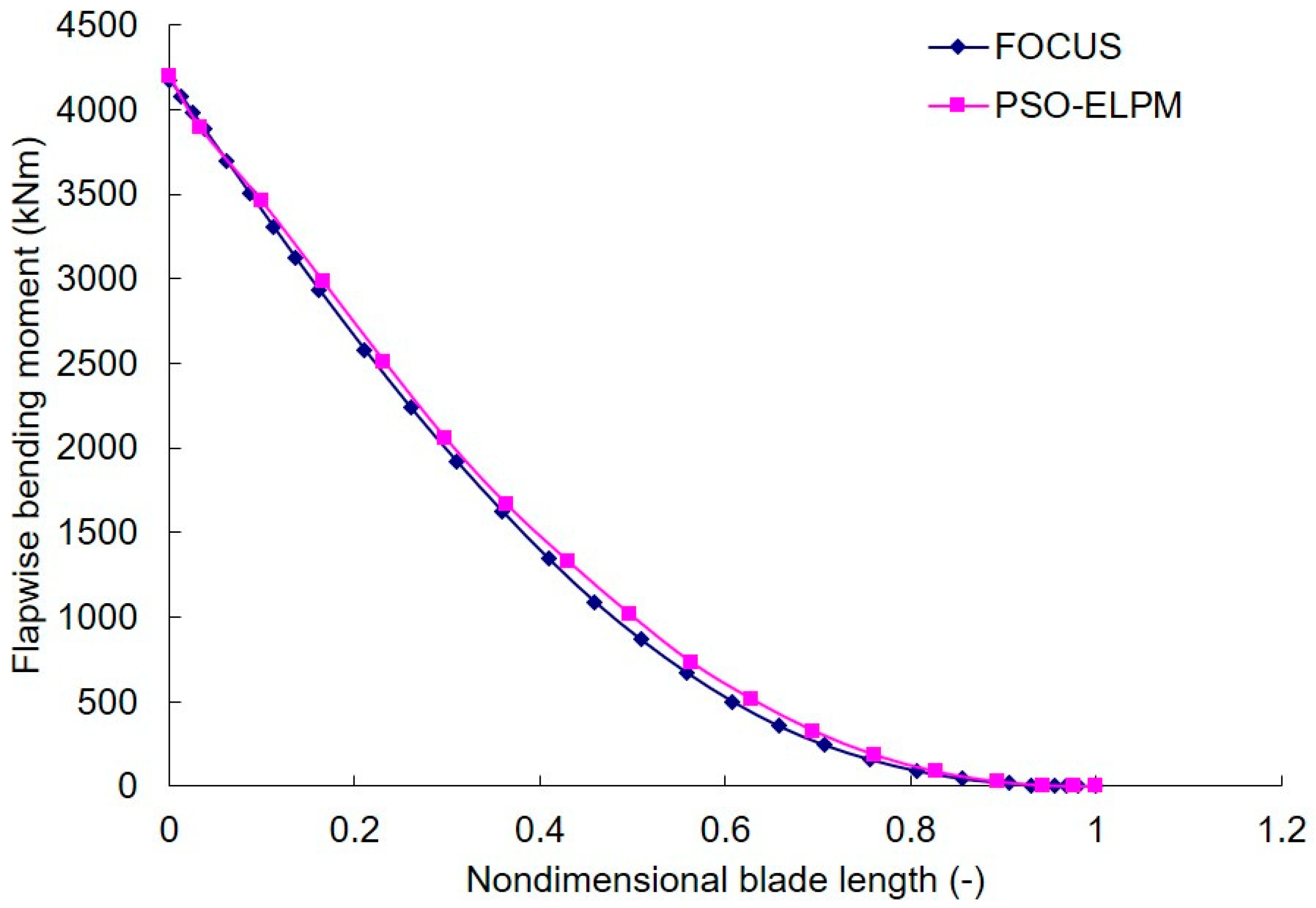
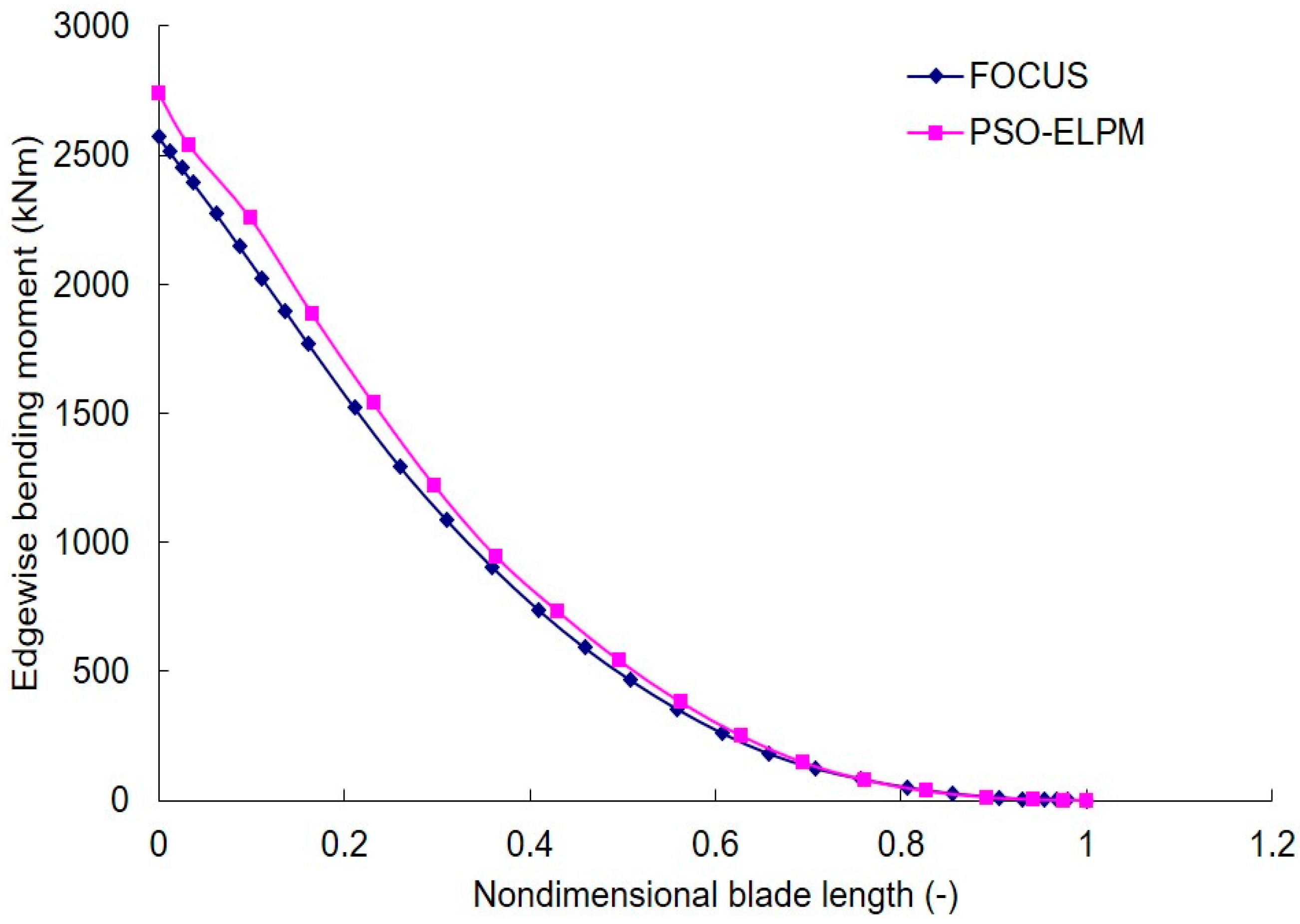
Though the extreme loads at the root can be used to evaluate whether the blade is overloading for the wind turbine, as well as the safety of the blade bolts, it is not enough for the preliminary blade preliminary. The load distribution along the blade span is also important. Luckily, this model can obtain the extreme load at any section. To further test it, the extreme load distributions for the 1.5 MW blade and 2.0 MW blade were obtained and compared with FOCUS results respectively in Figure 10, Figure 11, Figure 12 and Figure 13. The extreme loads were close at most sections for flapwise bending moments, though there was little difference in the middle of the blade in Figure 10 and Figure 12. From Figure 11 and Figure 13, we can see that the edgewise bending moment was also close at the blade tip, while there was obvious differences near the root. This method needs further improvements for edgewise load prediction. Overall, the PSO-ELPM model can accurately predict extreme bending moments in flapwise, which has the main influence on blade design. Maybe these loads can be used for evaluating the maximum blade deflection, which is a very important constraint for blade design. Moreover, from Table 2, we can see the extreme bending moments in edgewise happen at the maximum rotor speed. However, it is not easily determined due to . Maybe this is the reason why these loads cannot be accurately evaluated.
3.3. Effects of ΔΩ
Based on the above analysis, might have a significant effect on the extreme load prediction in this model. In this section, we want to test the results when is equal to 0, that is without delay in the safety control system. During the calculation, Equations (20) to (33) were still used. However, the upper value of rotor speed was change to 2.45 rad/s in Equation (26) and 2.17 rad/s in Equation (33) respectively. Figure 14, Figure 15, Figure 16 and Figure 17 show the comparison of results from PSO-ELPM with and without considering (expressed as “no delta omega” in these figures).
From Figure 14 and Figure 16, we can see the flapwise bending moments are still very close. It means had little influence on them. This is also can certified by Table 2. In Table 2, the extreme flapwise bending moment did not happen at the maximum rotor speed. Hence, the extreme value was not changed though the maximum rotor speed reduced. But the edgewise bending moments was very different, and noticeably changed without , especially near the blade root. Therefore, it needs further improvement. The should be fixed to make this model more accurate.
4. Conclusions
In this paper, so as to quickly solve the extreme loads and make it easily usable for preliminary blade design, a new simplified method, called as PSO-ELPM, was developed and validated in this study. Following this, the effects of the status parameters on the extreme loads were analyzed. Some conclusions are given below:
- The extreme root loads computed by PSO-ELPM and FOCUS were very close. The error between them was less than 10%. The extreme CMF_ROOT was lower than 5%. Moreover, PSO-ELPM needs much less computation cost than FOCUS. Hence, PSO-ELPM can be used for predicting the extreme load and is suitable for preliminary blade design.
- Higher rotor speed and smaller pitch angle will generate larger extreme bending moments at the root. It is for this reason that we need to pitch the blade to feather at high wind speed and activate security strategies when the rotor speed is larger than overspeed. In addition, negative yaw angle easily generates the extreme bending moments.
- When the control system is inactive, the extreme CMF_ROOT is increased but the extreme CME_ROOT is almost unchanged. It shows that the control system has significant influence on reducing the extreme loads, especially the extreme CMF_ROOT.
- By comparison of the extreme load distribution, flapwise bending moments are close to the results of FOCUS, while edgewise bending moments need be improved in the future.
- By the analysis of the effects of , there is little influence on the extreme flapwise bending moments. However, the edgewise bending moments change a lot while the maximum rotor speed reduces.
The PSO-ELPM model is a new method, which gives a different way to solve the extreme loads exerted on wind turbine blades. It has some advantages—it is simple and fast, but there are some aspects which have not been considered. There are also some defects that need to be further improved. For example, some parameters that change with the wind turbine model and not easily determined, and it needs to be fixed to make this model more generic. A further example is that the load calculation model needs to be improved so as to obtain better results. For example, the should be set as a variable changing with the wind speed. Storm conditions can be the most challenging conditions and should be added in the improved model. The load calculation could consider the aeroelastic effect. The should be fixed to make this model more accurate.
Author Contributions
C.L. developed the new method, did the numerical computation and wrote the article; K.S. supervised the work and did the results analysis; X.Z. discussed with the results and given some useful comments for writing.
Funding
This research was funded by the National Natural Science Foundation of China (No.51606196).
Acknowledgments
I would like to thank the China Scholarship Council (CSC) and the International Clean Energy Talent (iCET) Program.
Conflicts of Interest
The authors declare no conflict of interest.
References
- Wind Turbines—Part 1: Design Requirements, 3rd ed.; IEC 61400-1; International Electrotechnical Commission: Geneva, Switzerland, 2005.
- Rotor Blades for Wind Turbines; DNV GL AS, DNVGL-ST-0376; Det Norske Veritas Germanischer Lloyd Group: Arnhem, The Netherlands, 2015.
- LeRoy, M.F.; Steven, R.W. Predicting design wind turbine loads from limited data: Comparing random process and random peak models. In Proceedings of the 20th 2001 ASME Wind Energy Symposium, Reno, NV, USA, 11–14 January 2001. AIAA-2001-0046. [Google Scholar]
- Paul, S.V.; Sandy, B. Extreme Load Estimation for Wind Turbines: Issues and Opportunities for Improved Practice. In Proceedings of the 20th 2001 ASME Wind Energy Symposium, Reno, NV, USA, 11–14 January 2001. [Google Scholar]
- Patrick, J.M. Effect of turbulence variation on extreme Load prediction for wind turbines. J. Sol. Energy Eng. 2002, 124, 387–395. [Google Scholar]
- Pandey, M.D.; Sutherland, H.J. Probabilistic analysis of list data for the estimation of extreme design loads for wind turbine components. J. Sol. Energy Eng. 2003, 125, 531–540. [Google Scholar] [CrossRef]
- Fitzwater, L.M. Estimation of Fatigue and Extreme Load Distributions from Limited Data with Application to Wind Energy Systems; SAND 2004-0001; Sandia National Laboratories: Albuquerque, NM, USA; Livermore, CA, USA, 2004.
- Moriarty, P.J.; Holley, W.E.; Butterfield, S.P. Extrapolation of Extreme and Fatigue Loads Using Probabilistic Methods; Technical Report NREL/TP-500-34421; National Renewable Energy Laboratory NREL: Golden, CO, USA, 2004.
- Patrick, R.; Lance, M. Statistical Extrapolation Methods for Estimating Wind Turbine Extreme Loads. J. Sol. Energy Eng. 2008, 130, 031011. [Google Scholar]
- Puneet, A.; Lance, M. Simulation of offshore wind turbine response for long-term extreme load prediction. Eng. Struct. 2009, 31, 2236–2246. [Google Scholar]
- Jensen, J.J.; Olsen, A.S.; Mansour, A.E. Extreme wave and wind response predictions. Ocean Eng. 2011, 38, 2244–2253. [Google Scholar] [CrossRef]
- Wang, Y.; Xia, Y.; Liu, X. Establishing robust short-term distributions of load extremes of offshore wind turbines. Renew. Energy 2013, 57, 606–619. [Google Scholar] [CrossRef]
- Gong, K.; Ding, J.; Chen, X. Estimation of long-term extreme response of operational and parked wind turbines: Validation and some new insights. Eng. Struct. 2014, 81, 135–147. [Google Scholar] [CrossRef]
- Abdallah, I.; Natarajan, A.; Sørensen, J.D. Assessment of Extreme Design Loads for Modern Wind Turbines Using the Probabilistic Approach. Ph.D. Thesis, DTU Wind Energy, Roskilde, Denmark, 2015. [Google Scholar]
- Gordon, M.S.; Matthew, A.L.; Sanjay, R.A.; Spencer, H.; Andrew, T.M. Statistical Estimation of Extreme Loads for the Design of Offshore Wind Turbines During Non-Operational Conditions. Wind Eng. 2015, 39, 629–640. [Google Scholar]
- Lindenburg, C. PHATAS Release “NOV-2003” and “APR-2005” User’S Manual; ECN-I-05-005-r1; Knowledge Centre WMC: Wieringerwerf, The Netherlands, 2005. [Google Scholar]
- Bossanyi, E.A. GH Bladed Version 3.82 User Manual; Document: 282/BR/010; Garrad Hassan and Partners Limited: Bristol, UK, 2009. [Google Scholar]
- Liao, C.C.; Zhao, X.L.; Xu, J.Z. Blade Layers Optimization of Wind Turbines Using FAST and Improved PSO Algorithm. Renew. Energy 2012, 42, 227–233. [Google Scholar] [CrossRef]
- Croce, A.; Sartori, L.; Lunghini, M.S.; Clozza, L.; Bortolotti, P.; Bottasso, C.L. Lightweight rotor design by optimal spar cap offset. J. Phys. Conf. Ser. 2016, 753, 042003. [Google Scholar] [CrossRef]
- Pietro, B.; Carlo, L.B.; Croce, A. Combined preliminary-detailed design of wind turbines. Wind Energy Sci. 2016, 1, 71–88. [Google Scholar]
- Sartori, L.; Bellini, F.; Croce, A.; Bottasso, C.L. Preliminary design and optimization of a 20 MW reference wind turbine. J. Phys. Conf. Ser. 2018, 1037, 042003. [Google Scholar] [CrossRef]
- Bortolotti, P.; Bottasso, C.L.; Croce, A.; Sartori, L. Integration of multiple passive load mitigation technologies by automated design optimization-the case study of a medium-size on shore wind turbine. Wind Energy 2018, 22, 65–79. [Google Scholar] [CrossRef]
Figure 1.
Aerodynamic forces acting on a blade section.

Figure 2.
Pitch angle versus wind speed at hub center in some load cases.

Figure 3.
Pitch angle versus rotor speed in some load cases.

Figure 4.
(a) Power and (b) pitch angle changing with wind speed in steady simulation.

Figure 5.
Calculation method of Δβ2.

Figure 6.
Flow chart of the blade load calculation model.

Figure 7.
Flow chart of the particle swarm optimization-extreme load prediction model (PSO-ELPM).

Figure 8.
Iterative processes of variables: (a) Extreme CMF_ROOT calculation; (b) Extreme CMF_ROOT calculation for the 1.5 MW wind turbine blade.
Figure 8.
Iterative processes of variables: (a) Extreme CMF_ROOT calculation; (b) Extreme CMF_ROOT calculation for the 1.5 MW wind turbine blade.

Figure 9.
Iterative processes of variables: (a) Extreme CMF_ROOT calculation; (b) Extreme CMF_ROOT calculation for the 2.0 MW wind turbine blade.
Figure 9.
Iterative processes of variables: (a) Extreme CMF_ROOT calculation; (b) Extreme CMF_ROOT calculation for the 2.0 MW wind turbine blade.

Figure 10.
Comparison of extreme flapwise bending moment along the blade (1.5 MW).

Figure 11.
Comparison of extreme edgewise bending moment along the blade (1.5 MW).

Figure 12.
Comparisonof extreme flapwise bending moment along the blade (2.0 MW).

Figure 13.
Comparison of extreme edgewise bending moment along the blade (2.0 MW).

Figure 14.
Comparison of extreme flapwise bending moment along the blade (1.5 MW).

Figure 15.
Comparison of extreme edgewise bending moment along the blade (1.5 MW).

Figure 16.
Comparison of extreme flapwise bending moment along the blade (2.0 MW).

Figure 17.
Comparison of extreme edgewise bending moment along the blade (2.0 MW).


Table 1.
The extreme values of CMF_ROOT and CME_ROOT.
| 1.5 MW | 2.0 MW | |||||
|---|---|---|---|---|---|---|
| FOCUS | PSO-ELPM | Error | FOCUS | PSO-ELPM | Error | |
| CMF_ROOT (kNm) | 4176.45 | 4197.57 | 0.51% | 8084.68 | 7928.81 | −1.93% |
| CME_ROOT (kNm) | 2571.43 | 2741.36 | 6.61% | 4542.79 | 4352.48 | −4.19% |
Table 2.
Extreme bending moments and their corresponding status parameters with considering the constraint conditions about the βm.
Table 2.
Extreme bending moments and their corresponding status parameters with considering the constraint conditions about the βm.
| Bending Moment (kNm) | V1 (m/s) | Ω (rad/s) | β2 (°) | γ (°) | ψ (°) | ||
|---|---|---|---|---|---|---|---|
| 1.5 MW | CMF_ROOT | 4197.56 | 25.00 | 2.46 | 11.81 | −1.94 | 44.38 |
| CME_ROOT | 2741.36 | 29.13 | 2.84 | 32.48 | −8.00 | 67.83 | |
| 2.0 MW | CMF_ROOT | 7928.81 | 15.95 | 1.91 | 4.92 | −8.00 | 34.77 |
| CME_ROOT | 4352.48 | 38.87 | 2.45 | 90.00 | −8.00 | 340.68 | |
Table 3.
Extreme bending moments and their corresponding status parameters without considering the constraint conditions about the βm.
Table 3.
Extreme bending moments and their corresponding status parameters without considering the constraint conditions about the βm.
| Bending Moment (kNm) | V1 (m/s) | Ω (rad/s) | β2 (°) | γ (°) | ψ (°) | ||
|---|---|---|---|---|---|---|---|
| 1.5 MW | CMF_ROOT | 8328.10 | 38.26 | 2.84 | 3.50 | −8.00 | 25.90 |
| CME_ROOT | 2801.07 | 38.26 | 2.84 | 37.53 | −8.00 | 52.73 | |
| 2.0 MW | CMF_ROOT | 17877.90 | 38.87 | 2.45 | 7.20 | −8.00 | 16.34 |
| CME_ROOT | 4352.48 | 38.87 | 2.45 | 90.00 | −8.00 | 339.97 | |
© 2019 by the authors. Licensee MDPI, Basel, Switzerland. This article is an open access article distributed under the terms and conditions of the Creative Commons Attribution (CC BY) license (http://creativecommons.org/licenses/by/4.0/).
Share and Cite
MDPI and ACS Style
Liao, C.; Shi, K.; Zhao, X. Predicting the Extreme Loads in Power Production of Large Wind Turbines Using an Improved PSO Algorithm. Appl. Sci. 2019, 9, 521. https://doi.org/10.3390/app9030521
AMA Style
Liao C, Shi K, Zhao X. Predicting the Extreme Loads in Power Production of Large Wind Turbines Using an Improved PSO Algorithm. Applied Sciences. 2019; 9(3):521. https://doi.org/10.3390/app9030521
Chicago/Turabian StyleLiao, Caicai, Kezhong Shi, and XiaoLu Zhao. 2019. "Predicting the Extreme Loads in Power Production of Large Wind Turbines Using an Improved PSO Algorithm" Applied Sciences 9, no. 3: 521. https://doi.org/10.3390/app9030521
Note that from the first issue of 2016, this journal uses article numbers instead of page numbers. See further details here.