Nonlinear Extended-state ARX-Laguerre PI Observer Fault Diagnosis of Bearings


Department of Electrical, Electronics and Computer Engineering, University of Ulsan, Ulsan 44610, Korea
*
Author to whom correspondence should be addressed.
Appl. Sci. 2019, 9(5), 888; https://doi.org/10.3390/app9050888
Submission received: 21 December 2018
/
Revised: 24 February 2019
/
Accepted: 25 February 2019
/
Published: 1 March 2019
(This article belongs to the Special Issue Fault Detection and Diagnosis in Mechatronics Systems)
Abstract
:Featured Application
Fault diagnosis of industrial machines.
Abstract
This paper proposes an extended-state ARX-Laguerre proportional integral observer (PIO) for fault detection and diagnosis (FDD) in bearings. The proposed FDD technique improves fault estimation using a nonlinear function while generating a robust residual signal using the sliding mode technique, which can indirectly improve the performance of FDD. Experimental results indicate that the system modeling error in a healthy condition is less than 2.5 × 10⁻¹⁰ N.m. In the next step, the ARX-Laguerre PIO is designed to define the state and output of the system observer. The high gain extended-state observer is designed in the third step to estimate the mechanical (bearing) faults based on the nonlinear function. In the last step, robust residual signals are generated based on the sliding mode algorithm for accurate fault identification. This approach improves the performance of an ARX-Laguerre linear PIO method. Employing the proposed method, we demonstrate that in the presence of uncertainties and disturbances, the ball, inner, outer, inner-ball, outer-ball, inner-outer, and inner-outer-ball failures with various motor torque speeds (300 RPM, 400 RPM, 450 RPM, and 500 RPM) and crack sizes (3 mm and 6 mm) are detected, identified, and estimated efficiently. The effectiveness of the proposed technique is compared with an ARX-Laguerre proportional integral observation (ALPIO). Experimental results indicate that the proposed technique outperforms the ALPIO technique, yielding 17.82% and 16.625% performance improvements for crack sizes of 3 mm and 6 mm, respectively.
1. Introduction
Induction motors have been used in diverse industries, such as the machine tool and oil industries. The dynamic behavior of an induction motor is entirely nonlinear, which can cause various challenges in control and fault diagnosis. High-temperature environments, heavy-duty cycles, poor installation, overloading, and aging of components cause a diverse range of electrical and mechanical defects in motors. Diverse faults have been defined in induction motors, such as motor failures, air-gap faults, bearing and cage faults, and stator failures. The two main types of induction motor defects are mechanical and electrical failures. Various types of induction motor faults are mostly associated with mechanical defects (79%), such as bearing defects (69%) and rotor faults (10%). The other types of induction motor faults are electrical failures (21%), such as open circuits and short circuits in stator windings [1].
The most common defect in induction motors are mechanical failures. These faults are classified as bearing faults and rotor faults. Across industries, bearing defects are the most common critical effect increasing failure in induction motors [1]. The four main types of bearing defects are inner raceway faults, outer raceway faults, ball failures, and cage faults [2,3]. To analyze the condition of bearings, different types of condition monitoring techniques, such as acoustic emission (AE), stator current, shaft voltage, bearing circuit, and vibration analysis, have been reported in the literature [4]. Vibration and AE measurement techniques are the most widely used for monitoring the bearing conditions [4]. Since AE signals are strongly correlated with actual faults, this research utilizes acoustic emission sensors for data collection.
Two main fault detection and diagnosis methods are hardware-based fault detection and diagnosis (FDD) and functional-based FDD [5]. Fault detection and identification based on the hardware method is a stable, reliable, and preventive maintenance technique, but it is also expensive. To address this issue, functional-based FDD has been presented [6,7,8,9,10,11,12,13,14,15,16,17,18]. The four foremost types of functional-based fault detection and diagnosis are signal-based FDD [6,7,8,9,10,11], knowledge-based FDD [12,13], model-based FDD [14,15,16], and hybrid-based FDD [17,18]. Several signal-based techniques, such as motor current signature analysis (MCSA), vibration analysis, the noise monitoring technique, and torque monitoring analysis, have been introduced. A common signal-based technique for FDD in the induction motor is the MCSA technique. This technique is more common for broken rotor bar (BRB) faults, air-gap eccentricity faults, and stator electric current faults. To diagnose faults in the mechanical parts of an induction motor, such as a bearing, vibration and acoustic emission analysis are more common [7]. The main drawbacks of signal-based FDD are reliability and robustness. Knowledge-based FDD has various advantages, but this technique needs massive quantities of data for training [19]. Model-based FDD has been considered a robust and reliable FDD technique.
The main concept of model-based FDD is system modeling, which has been acknowledged by several researchers in the field [19]. The main techniques for model-reference FDD use output observers, system identification and parameter estimation, and the parity equation [20,21]. Various researchers have used observational methods for FDD, such as a proportional integral (PI) observer [22], proportional multiple integral (PMI) observer [23] and sliding mode observer (SMO) [24]. The fault diagnosis in noisy conditions and state-estimation in the highly nonlinear systems are the main drawbacks in the PI and PMI observers. The sliding mode observer has been considered to solve the linear observer’s drawback [24]. Apart from several advantages of the sliding mode observer, chattering phenomenon is the main drawback. The higher order sliding mode observer (HOSMO) was presented to solve the chattering phenomenon in the sliding mode observer [25]. This observer works based on the system’s dynamic behavior, and thus the observer performance can be significant if most system dynamic parameters are known. To address the challenges of proportional integral observer (PIO) and SMO, the sliding mode extended-state ARX-Laguerre PI observer technique is introduced in this research. This technique is designed with the following steps. In the first step, the ARX-Laguerre technique is used for the system (induction motor) modeling. In the second step, the first observer (ARX-Laguerre PI observer) is designed for system and fault estimation. Apart from the numerous positive attributes of the ARX-Laguerre PI observer, this technique has an issue of fault estimation accuracy. To improve fault estimation based on the ARX-Laguerre PI observer, in the next step, an extended-state ARX-Laguerre PI observer is used. Based on this method, the performance of fault estimation increased sharply. The residual generation plays a vital role in the observer-based fault diagnosis. To generate a robust residual signal, in the fourth step, the sliding mode technique is utilized. This method is robust and effective for motor fault diagnosis at variable speeds. To process the threshold value, in the fifth step, a robust sliding mode technique is used. After processing the robust residual signal and the threshold value, in the sixth step, the proposed extended-state ARX-Laguerre PI observer generated two different scenarios for fault diagnosis: (a) variable crack sizes and (b) variable motor speeds. This paper presents three different problems and the solutions to solve these problems. The problems and solutions are briefly described as follows:
Problem 1: System (induction motor) modeling is a significant issue, especially to the design model-reference technique for FDD.
Solution 1: The robust system estimation technique based on the ARX-Laguerre technique is employed for system estimation (please see Section 4.1).
Problem 2: Fault detection based on the proposed method in the presence of unknown parameters.
Solution 2: After designing the proposed method, robust sliding mode residual generation is introduced to find the robust residual signal and generate it. Based on the comparison between the band of uncertainty and threshold value, the abnormal condition can be detected, as seen in Section 4.3.
Problem 3: Fault identification and estimation are the third issue of this research.
Solution 3: For fault estimation and identification, the proposed extended-state observer is used to improve the performance of the proposed ARX-Laguerre PIO and reduce the effect of uncertainty (Section 4.4).
The rest of this paper is organized as follows: Section 2 gives the dataset. Section 3 presents the problem statements and the proposed method objectives. Section 4 introduces the proposed nonlinear extended-state ARX-Laguerre PI observer method and the effectiveness of the proposed method for fault detection and diagnosis. Section 5 shows the results and discussions, and Section 6 concludes this paper.
2. Dataset
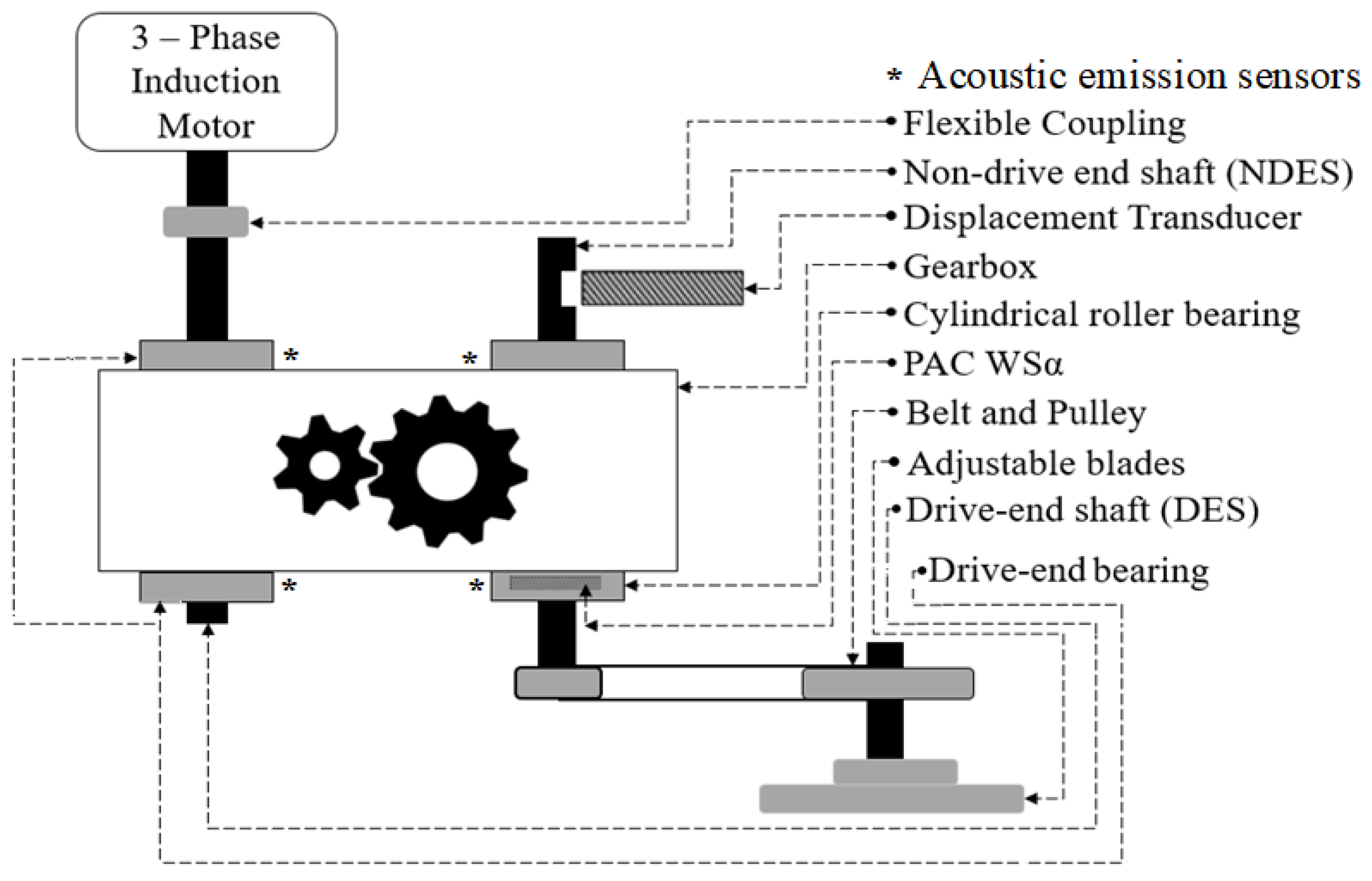
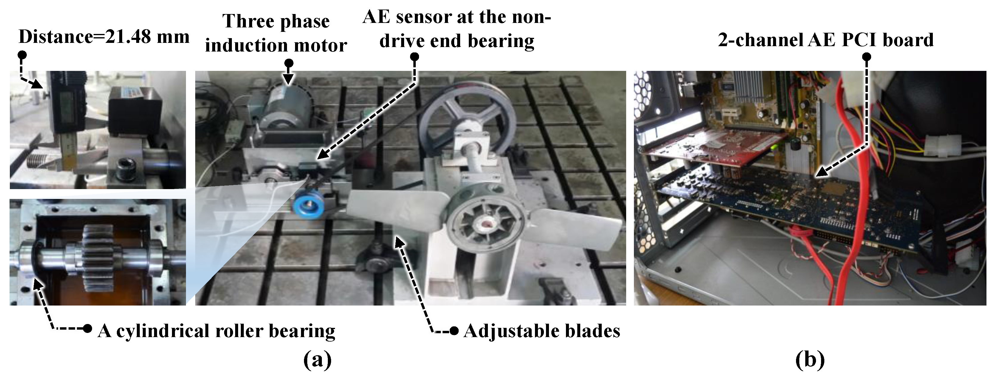
Figure 1 demonstrates an experimental system for the fault simulator of bearings. To transfer the torque to the no-drive-end shaft (NDES) through the gearbox, the three-phase induction motor is connected to the drive-end shaft (DES) [26]. Figure 2 illustrates the experimental data acquisition system to extract the normal and faulty signals.
Faults with crack sizes of 3 mm and 6 mm in diameter are seeded on the drive-end bearings as the outer raceway fault (O), inner raceway fault (I), ball raceway fault (B), inner-outer raceway fault (IO), inner-ball raceway fault (IB), outer-ball raceway fault (OB), and inner-outer-ball raceway fault (IOB) (see Figure 3). The data are recorded at 250 kHz sampling rate and the rotational speeds are 300, 400, 450, and 500 RPM. The details of the data are given in Table 1.
3. Problem Statements and Proposed Method Objectives
The principal target of this paper is to detect and estimate an induction motor’s mechanical faults based on the extended-state ARX-Laguerre PI observer. The foremost issue of the induction motor is mathematical modeling in the presence of uncertainties and faults. Thus, this paper utilizes a state-of-the-art induction motor experiment for modeling based on system identification. The three-phase space vector of induction motor formulation based on the stator and rotor voltage, current, and flux are presented below [1,27]:
where and are the three phase stator voltage, three phase rotor voltage, stator impedance, rotor impedance, three phase stator current, three phase rotor current, change of stator flux, and change of rotor flux, respectively. The flux linkage can be written as follows:
Here, and are the stator flux, rotor flux, stator inductance matrix, rotor inductance matrix, and stator-rotor mutual inductance, respectively. Based on (1) and (2), the stator and rotor currents are calculated as follows:
where is rotor rectangular velocity. Based on the dynamic formulation of an induction motor, mathematical modeling of the induction motors is incredibly complicated and uncertain, and thus, the task of modeling is significantly important. To address this issue, this research utilizes an ARX-Laguerre system estimation technique for system modeling. This technique reduces the complexity and improves the robustness [28]. After modeling healthy and faulty conditions, the extended-state ARX-Laguerre PI observer can be designed for fault detection and diagnosis. A block diagram of the proposed method is depicted in Figure 4.
4. Proposed Fault Detection and Diagnosis
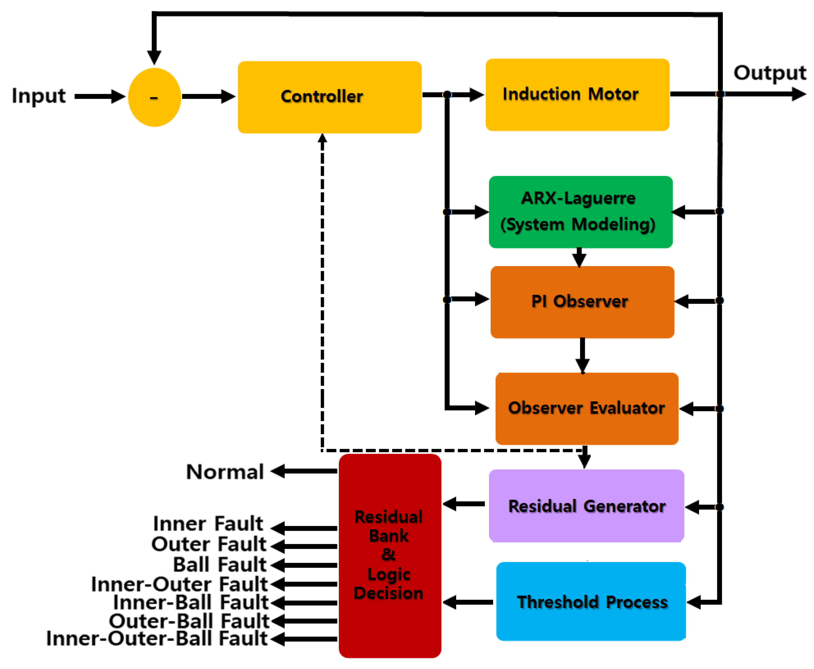
An induction motor is a significant system in various industries. Reliable induction motor fault detection and diagnosis is significant for maintaining machine operations in safety conditions. A problem arises in most of the industrial systems in using model-free techniques (knowledge-based and signal-based) to detect, estimate, and identify faults, especially under uncertain and noisy conditions. To address this issue, an extended-state ARX-Laguerre PI observer is proposed in the following section. Figure 5 illustrates the proposed mechanism for bearing fault diagnosis. ARX-Laguerre system modeling is the first step for model-reference fault diagnosis.
4.1. ARX-Laguerre System Modeling
As shown in Figure 5, the first step to design a model-reference observer is system modeling. This step is important to design an accurate observer for fault diagnosis. Based on the proposed method, this system is modeled by the ARX-Laguerre technique. The proposed method is robust in the presence of motor speed variation. When the motor speed changes, the system’s model is changed, and the proposed observer detects the model’s change. The filter network ARX-Laguerre orthonormal technique for modeling an induction motor is presented based on the system input and output, Fourier coefficients, and Laguerre-based orthonormal function as follows [28]:
where , and are the system output, coefficients of Fourier, order of system, functions of the Laguerre-based orthonormal, Laguerre poles, convolution product, system input, output signal filtered, and filtered input signal, respectively. To calculate the state-space equation, the following variables are defined in Equations (5) and (6).
Based on Equations (4)–(6) the ARX-Laguerre technique is represented as
Here, and are two polynomials with degrees and , respectively. Based on Equation (7) the transfer function is represented as follows:
The identification between Equations (6) and (7) provides (9).
Based on Equations (5), (6), (7), and (9) the optimization problem is defined as follows [28]:
From the relations Equations (5), (6), and (9), the minimization technique Equation (10) is used to decompose the polynomials and on the Laguerre orthonormal bases, and the and are optimized. A block diagram of the ARX-Laguerre technique is illustrated in Figure 6. The ARX-Laguerre state-space equation is written as follows:
where and are the system state, coefficient matrices, measured output, control input, uncertainty and disturbance, faults, and the Fourier coefficient, respectively. Based on Figure 3, seven types of faults are defined as inner fault , outer fault , ball fault , inner-outer fault , inner-ball fault , outer-ball fault , and inner-outer-ball fault . are presented in Equations (12), (13), (14), (15) and (16), respectively.
Here, A0 and Ai are defined in Equations (13) and (14), respectively
where and are null matrices of the dimensions and . and are defined as follows:
Here, , , , , , , and . is optimized via a gradient descent (GD) optimization method using the following equations:
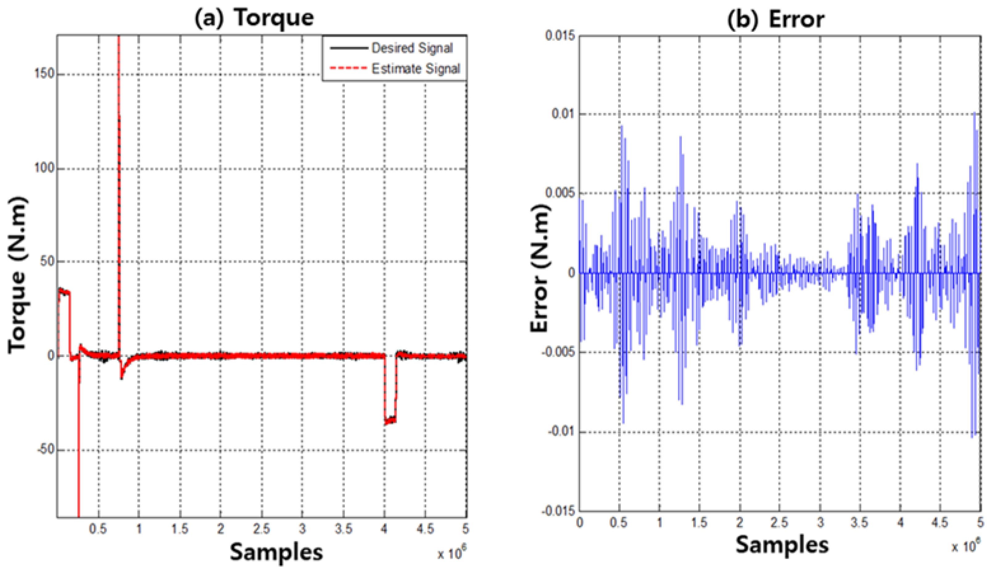
Here, is the covariance matrix and is the error prediction. Figure 7 and Figure 8 illustrate the estimation accuracy for the healthy and faulty conditions using the ARX-Laguerre method. For the healthy state in Figure 7, the sensitivity of the torque estimation is exceptionally high, and the rate of error is close to zero. In the faulty condition, the error rate increases, which causes an increase in the residual signal which is generated by the sliding mode technique. Figure 8 illustrates the power of the estimated signal and error rate in the faulty condition.
4.2. Extended-State ARX-Laguerre PI Observer
The proposed methodology comprises of six major parts, as shown in Figure 5: (a) system modeling using the ARX-Laguerre technique, (b) proportional-integral (PI) observer, (c) observer evaluator, (d) residual generator, (e) threshold process, and (f) residual bank and logic decision. The classical ARX-Laguerre PI observer offers a linear approach to find an optimized estimation of the system and fault. This technique is stable, but it has an issue regarding accurate fault estimation and robustness. To evaluate the ARX-Laguerre PI observer, a sliding mode extended-state observer is considered. This technique improves the robustness and precision of fault estimation. Using ARX-Laguerre state space system modeling, the ARX-Laguerre PI observer method is defined to estimate the system modeling output and fault. Therefore, the block of the PI observer is defined as the following equation.
where and are the state estimated, output estimated, faults estimated, and the proportional coefficient, respectively. Based on bearing conditions, the fault estimation can be estimated in seven different conditions such as inner fault , outer fault , ball fault , inner-outer fault , inner-ball fault , outer-ball fault , and inner-outer-ball fault . The future state of PIO is a function of the current state, current output, current input, faults, disturbance, and current error of the signal. For fault estimation using the ARX-Laguerre PIO technique, the integral term is used to reduce the fault estimation error. The integral term of fault estimation in the ARX-Laguerre PI observer is given in Equation (12).
Here, is the integral term coefficient. Using Equation (18), the inner, outer, ball, inner-outer, inner-ball, outer-ball, and inner-outer-ball faults are estimated based on the integral term. Using this technique, the future faults are estimated by the current fault and error of the signal. This technique has been used in several applications [28], but it has a drawback in the presence of uncertain and noisy conditions. To address this issue, an observer evaluator is considered, as shown in Figure 5. The extended-state ARX-Laguerre PI observer is designed to improve the performance of faults estimation. Therefore, the observer evaluator block, as shown in Figure 5, is defined as the following two Equations, (13) and (14):
Here, and are the extended-state coefficients. Based on bearing conditions, the fault estimation can be estimated in seven different conditions such as inner fault , outer fault , ball fault , inner-outer fault , inner-ball fault , outer-ball fault , and inner-outer-ball fault . According to Equations (19) and (20), the system’s output and faults are estimated using the extended-state ARX-Laguerre PI observer. This technique is more accurate and robust than the ARX-Laguerre PI observer technique. The stability and convergence are proven in the Appendix [29]. After designing the proposed extended-state ARX-Laguerre PI observer method, the residual generator is designed. The residual generation block has two inputs: (a) the system’s output and (b) the system’s estimation output. The robust sliding mode technique is used to generate reliable residual signals [30]. This technique is defined as the following equation.
Here, and are the output’s error, switching function, sliding gain, and residual signal, respectively. After designing the proposed extended-state ARX-Laguerre PI observer and residual generator, in the next step, the sliding mode threshold process evaluation is proposed [29]. As shown in Figure 5, this block has two inputs: (a) the system’s modeling output and (b) the system’s estimation output, which is represented by the proposed method. Using the robust sliding mode method, the threshold value for different conditions (e.g., normal state and faulty conditions) is calculated by the following equation [30]:
where and are sliding surface, output’s change of error, sliding surface slope, sliding gain, and threshold value, respectively. As shown in Figure 5, the last block for fault detection and fault diagnosis using the proposed method is residual bank and logic decision. This block is divided into two main parts: (a) fault detection and (b) fault diagnosis.
4.3. Fault Detection
As shown in Figure 5, the residual bank and logic decision block has two inputs from the residual generator and threshold process. Using Equations (21) and (22) for fault detection, we have two different conditions: (a) healthy condition and (b) faulty condition . The threshold level for normal condition is defined by . When the system works in a healthy condition , the normal residual signal is
When the system works in a faulty condition , the faulty residual signal is
Using Equations (23) and (24), faults can be detected.
4.4. Fault Identification
The main part of fault identification is fault estimation. The residual bank is evaluated using the fault estimation. The two blocks for fault estimation include (a) the PI observer block and (b) the observer evaluate block. In the first step, the ARX-Laguerre PI observer is designed, (17). In this step, a fault is estimated by an integral linear function, (18). To evaluate the accuracy of fault estimation, the extended-state ARX-Laguerre PI observer is considered, (21). After accurate fault estimation, the next step is fault identification. As shown in Figure 5, for fault identification, three important blocks are: (a) the threshold process block, (b) the residual generator, and (c) residual bank and logic decision. The main idea of the threshold process is generated in (22). Regarding (20) and (21), seven different faulty conditions have been defined in this research, i.e., ball, inner, outer, inner-ball, outer-ball, inner-outer, and inner-outer-ball faults. Based on Equation (22) to detect the level of faults, the following equations are represented [30]:
Here, and are defined as the outer fault threshold, inner fault threshold, ball fault threshold, outer-ball fault threshold, inner-ball fault threshold, outer-inner fault threshold, outer-inner-ball fault threshold, coefficients, and surface slope coefficients, respectively. The last step for fault diagnosis is logic decision, as shown in Figure 5. This block is used for fault identification and isolation. This block has two inputs: (a) residual generation and (b) threshold process. The residual signals and threshold levels are calculated by (21) and (22), respectively. The following equation is used for the condition decision.
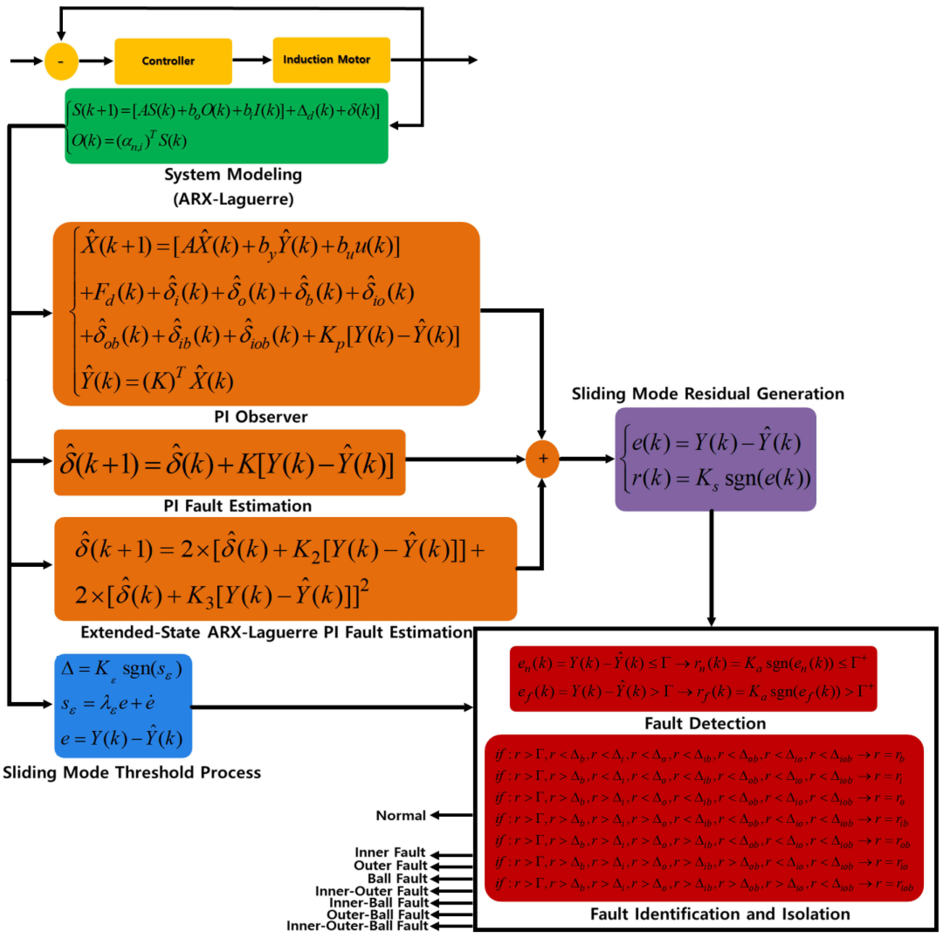
Here, and are the ball fault residual signal, inner residual, outer residual, inner-ball residual, outer-ball residual, inner-outer fault residual, and inner-outer-ball residual, respectively. Based on Equation (32), faults are isolated whenever the residuals overshoot their corresponding thresholds . Algorithm 1 illustrates the extended-state ARX-Laguerre PI observer for fault diagnosis of an induction motor. The block diagram of mechanical fault detection and diagnosis illustrates in Figure 9. In this technique, the abnormal signal is highly sensitive to the residual signals in normal or faulty conditions, and it is robust to the other faults and noises.
| Algorithm 1. Extended-state ARX-Laguerre PI observer for fault diagnosis of an induction motor | |
| 1: | Perform system modeling based on the ARX-Laguerre technique (4,11) |
| 2: | Run the ARX-Laguerre PI observer (17) |
| 3: | Run the observer evaluator based on the extended-state method (20) |
| 4: | Run the proposed method for fault estimation (19,20) |
| 5: | Run the residual generator based on the sliding mode technique (21) |
| 6: | Run the threshold value based on the sliding mode technique (22) |
| 7: | Run the decision logic for fault detection (23,24) |
| 8: | Run the decision logic for fault identification (32) |
5. Results and Analysis
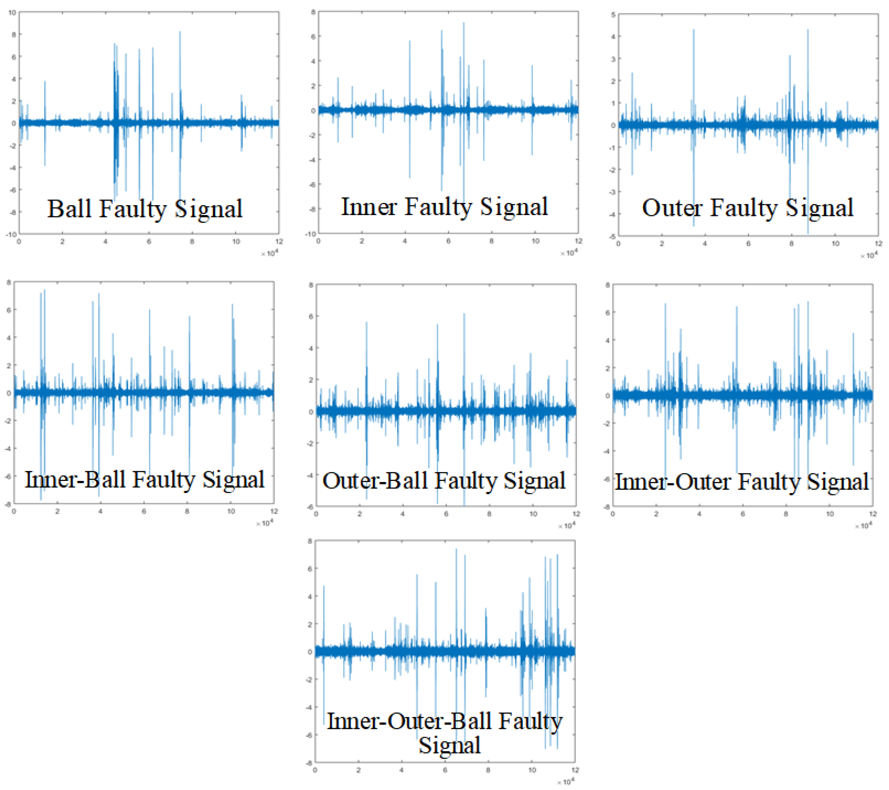
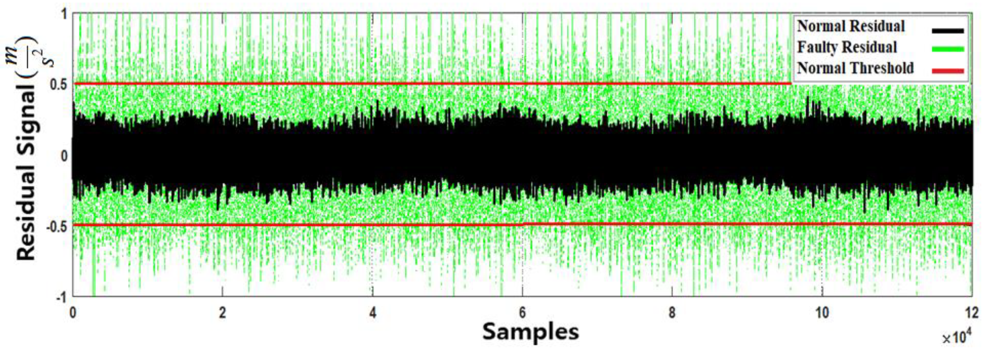
The effectiveness of the proposed extended-state ARX-Laguerre PI observer for the identification of various conditions (e.g., normal, inner, outer, ball, inner-ball, outer-ball, inner-outer, and inner-outer-ball) is compared to the ARX-Laguerre PI observer. The raw signal for different faulty conditions is illustrated in Figure 10. Regarding (32), the absolute of threshold values for dataset 4 for normal, ball, inner, outer, inner-ball, outer-ball, and inner-outer conditions are 0.5, 1, 2, 3, 4, 6, and 8, respectively. The absolute of residual signal for dataset 4 for normal, ball, inner, outer, inner-ball, outer-ball, inner-outer, and inner-outer-ball conditions are , respectively. Figure 11 illustrates the accuracy of the fault detection using dataset 4. As shown in Figure 11, the faulty signal can be detected easily.
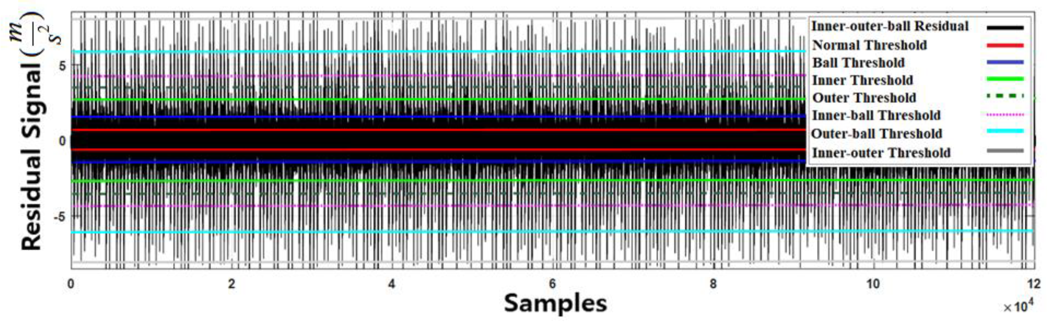
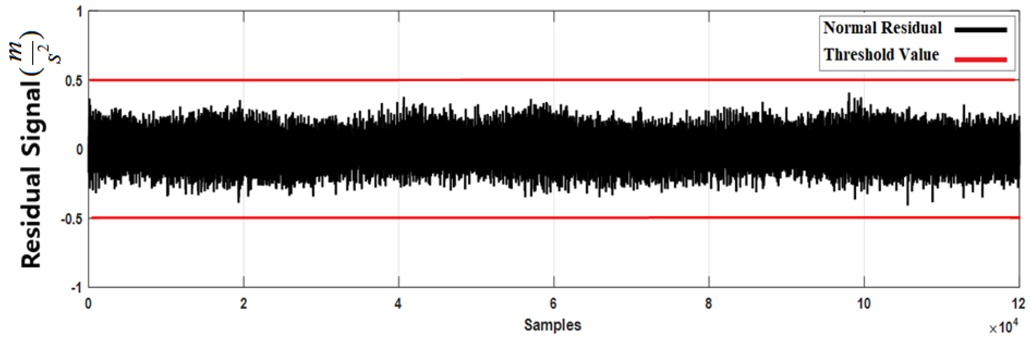
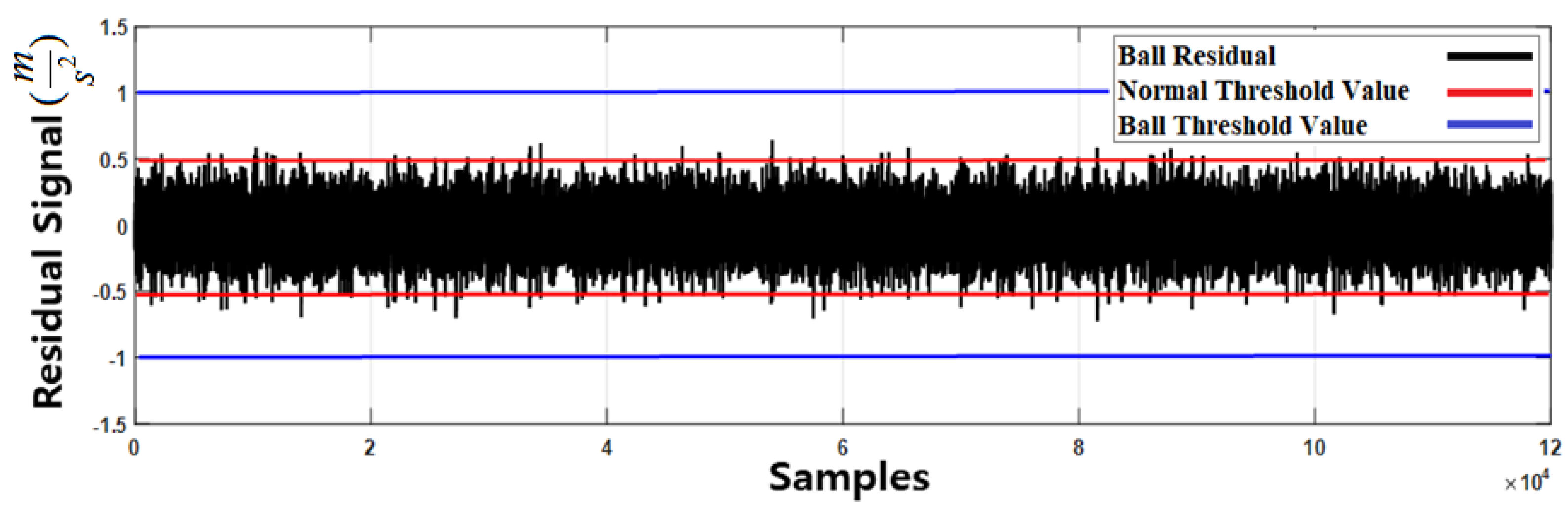
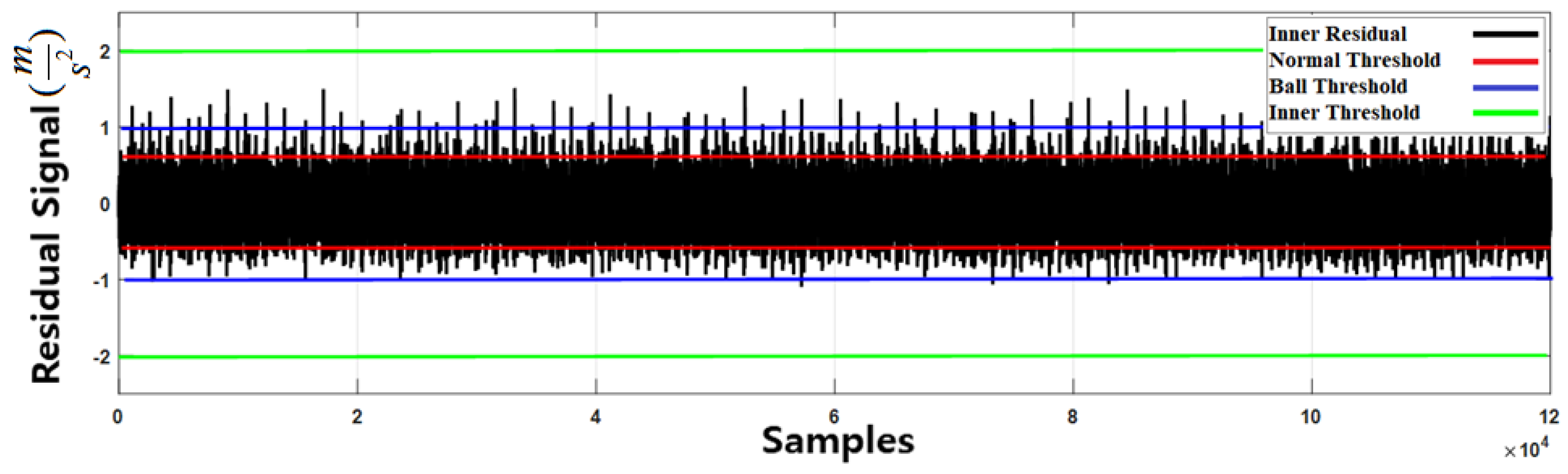
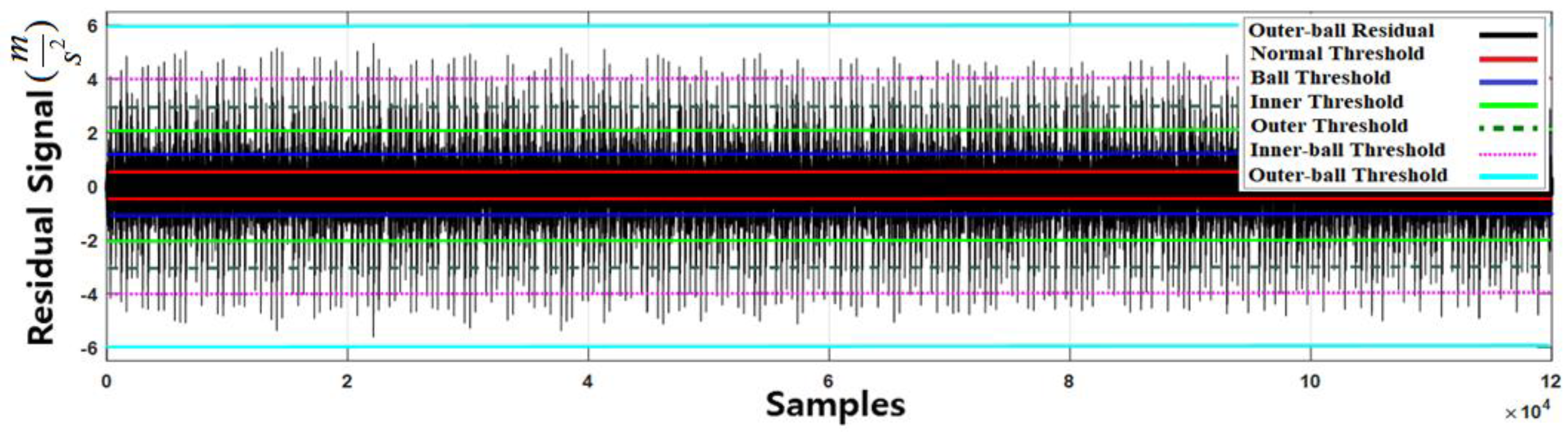
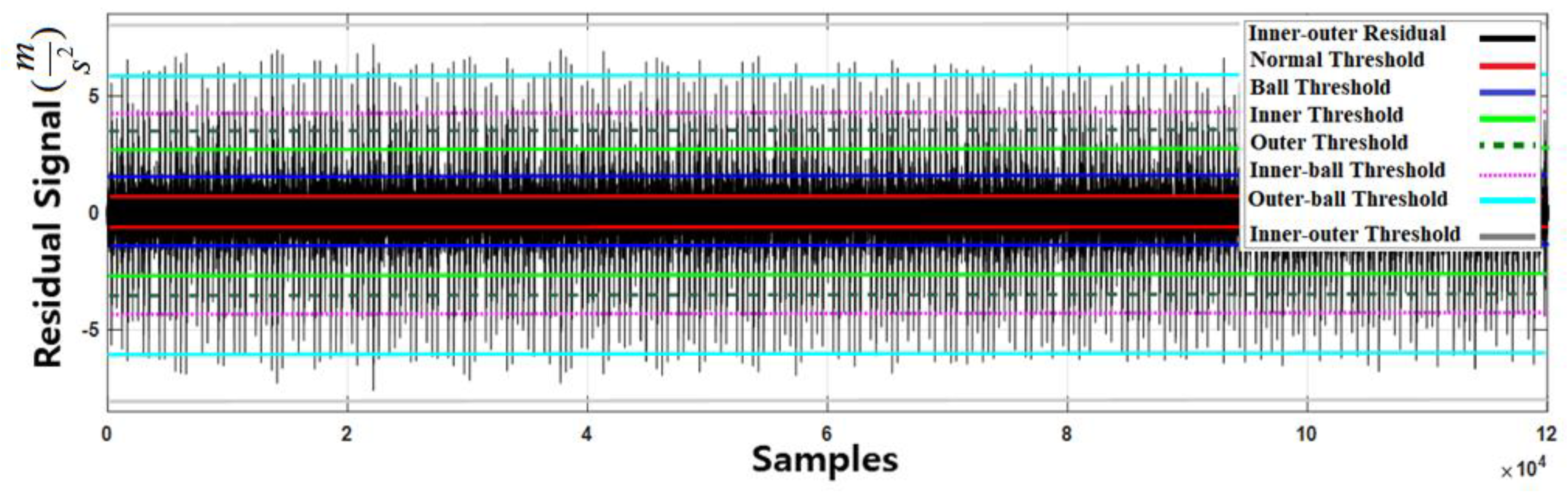
Figure 12, Figure 13, Figure 14, Figure 15, Figure 16, Figure 17, Figure 18 and Figure 19 illustrate fault diagnosis for various conditions. Figure 12 illustrates the normal signal identification for dataset 4. Figure 13 shows ball fault identification for dataset 4. In this figure, the ball residual signal is lower than the ball threshold value. Figure 14, Figure 15, Figure 16, Figure 17, Figure 18 and Figure 19 illustrate the fault diagnosis for outer, inner-ball, outer-ball, inner-outer, and inner-outer-ball, respectively. As shown in Figure 14, in some samples, the inner residual signal level is higher than the ball threshold value, which can be used for fault diagnosis and fault isolation. In the experiment, we have 120,000 samples for each condition for all datasets. Dataset 4 is used as a training dataset to adjust the threshold. The other datasets (dataset 1, dataset 2, and dataset 3) are used as a test. Figure 12 shows normal condition, and level of the residual signal is less than the normal threshold value. It means that in this state, the proposed method accurately detects the normal condition. For the faulty ball condition, the level of a residual signal is more prominent than the normal threshold and lower than ball fault threshold. Therefore, for the faulty ball condition, the residual signal should be between normal threshold and ball threshold. In this technique, 100 windows are defined for testing for various types of datasets, where 1200 samples are used in the window. Figure 15 illustrates the residual signal and threshold value of the outer defect for fault diagnosis using the proposed method. Whenever the level of the outer signal is higher than the inner threshold value, fault can be isolated. Figure 16, Figure 17, Figure 18 and Figure 19 illustrate the fault diagnosis for the inner-ball, outer-ball, inner-outer, and inner-outer-ball for dataset 4.
Table 2, Table 3, Table 4 and Table 5 illustrate the accuracy of fault diagnosis using the proposed extended-state ARX-Laguerre PI observer and ARX-Laguerre PI observer for the normal condition, faulty ball state, inner fault, outer fault, inner-outer fault, inner-ball fault, outer-ball fault, and inner-outer-ball fault, respectively. The diagnostic accuracy is reported as a percentage of correct fault identification in all data.
As shown in Table 2, Table 3, Table 4 and Table 5, the average rate of failure identification is 98.8% for the proposed extended-state ARX-Laguerre PIO and 80.5% for the ARX-Laguerre PI observer.
The proposed extended-state ARX-Laguerre PI observer fault diagnosis method outperforms the state-of-the-art ARX-Laguerre PI observer method, yielding an average performance improvement of 17.82%, and 16.625% for 3 mm and 6 mm cracks, respectively. Overall, the proposed extended-state ARX-Laguerre PI observer fault diagnosis method efficiently identifies single and composite faults in an induction motor.
To analyze the false alarm in the proposed algorithm, the confusion matrix using dataset 2 is illustrated in Table 6 and Table 7. Based on Table 6, for normal condition, apart from the precision is 100% but recall is 97.1% because proposed method cannot predict all normal case correctly. The main target to design the classifier is improving the performance of recall and precision, as well. Regarding Table 6 and Table 7, the overall accuracy for 3 mm crack size is 95.07% and for 6mm crack size is 98.13%. In this experiment, the bearing data are collected under four different motor speeds, as shown in Table 1. Using the proposed method, this system is modeled by the ARX-Laguerre method. The proposed method is robust even if the motor speed changes. When the motor speed changes, the system model is changed, and the proposed observer detects the model change. This technique is robust, and the speed variation is defined as an uncertainty condition.
Table 8 and Table 9 present the fault diagnosis accuracy for variable motor speeds (e.g., 300 RPM, 400 RPM, 450 RPM, and 500 RPM) in different crack sizes (e.g., 3 mm and 6 mm), various conditions (normal, ball fault, inner fault, outer fault, inner-outer fault, inner-ball fault, outer-ball fault, and inner-outer-ball fault) of the proposed method and PIO. Dataset 4 is used to calculate the threshold value for different types of faults and two crack sizes.
6. Conclusions
In this paper, the proposed extended-state ARX-Laguerre PI observation technique was evaluated to detect, estimate, and classify several faults in a bearing including ball, inner, outer, inner-ball, outer-ball, inner-outer, and inner-outer-ball faults. In the first step, the ARX-Laguerre method was introduced for system modeling and estimation. To increase the accuracy of fault detection and diagnosis, the proposed extended-state ARX-Laguerre PI observer was designed in the next step. Experimental results showed that average performance improvements using the proposed method are 17.62% and 16.626%, as compared with the ARX-Laguerre PI observer technique for 3 mm and 6 mm bearing crack damage, respectively.
Author Contributions
All of the authors contributed equally to the conception of the idea, the design of experiments, the analysis and interpretation of results, and the writing of the manuscript.
Acknowledgments
It was funded by The Leading Human Resource Training Program of the Regional Neo Industry through the National Research Foundation of Korea (NRF) funded by the Ministry of Science, ICT and Future Planning (NRF-2016H1D5A1910564).
Conflicts of Interest
The authors have no conflicts of interest to declare.
Nomenclature
| Stator voltage matrix | Stator inductance matrix | ||
| Rotor voltage matrix | Rotor inductance matrix | ||
| Stator impedance matrix | Stator and rotor mutual inductance | ||
| Rotor impedance matrix | Rotor rectangular velocity | ||
| Flux and Flux derivation for stator | System’s output | ||
| Flux and Flux derivation for rotor | Fourier coefficients | ||
| Stator current | System’s order | ||
| Rotor current | Laguerre-based orthonormal | ||
| Laguerre pole | * | Convolution product | |
| Systems input | Input and Filter output signal | ||
| Filter input signal | System’s state | ||
| Uncertainty and disturbance | Faults | ||
| Coefficient matrices | Fourier coefficient | ||
| Null matrices | Estimation vector | ||
| Inner fault | Outer fault | ||
| Ball fault | Inner-ball fault | ||
| Inner-outer fault | Outer-ball fault | ||
| Inner-outer-ball fault | Coefficients | ||
| Sliding Mode Coefficients | Error | ||
| Fourier coefficient | Threshold Value | ||
| Residual signal | Normal residual signal | ||
| Faulty residual signal | Normal threshold level | ||
| Estimation of the system’s state | Estimation of the system’s output | ||
| Residual signal in various states | Threshold value in various states | ||
| Sliding surface | Sliding surface slope coefficients | ||
| Fault estimation function | Fault estimator by PIO (proportional integral observer) | ||
| Convergence time | Positive constant |
Appendix A
The stability and convergence of the proposed extended-state ARX-Laguerre PI observer technique is proven in the following part.
Proof: if the extended-state observer is defined by the following Equation:
In the normal condition (), the convergence reaching time is calculated based on (A-3).
Based on [29], in the first step, we defined the convergence time in the normal condition, Equation (A-4). Based on Equation (A-4), the residual signal is converged to zero in a finite time. In the abnormal condition, the compensate variable is defined by
Based on [29], to have stability and finite time convergence, the coefficient is bounded as follows:
Based on the Lyapunov theorem, the Lyapunov of the proposed observer is defined by the following Equation:
The derivative of the Lyapunov function is defined by Equation (A-7).
The band of the fault estimation based on the proposed method is defined by the following assumption:
Based on Equation (A-7) and Equation (A-8),
So, if , . Based on [29], when , the residual signals converge to zero in a finite time.
References
- Duan, F. Induction Motor Parameters Estimation and Faults Diagnosis Using Optimisation Algorithms. Ph.D. Thesis, School of Electrical and Electronic Engineering, University of Adelaide, Adelaide, Australia, 2015. [Google Scholar]
- Shao, H.; Jiang, H.; Zhang, H.; Liang, T. Electric locomotive bearing fault diagnosis using a novel convolutional deep belief network. IEEE Trans. Ind. Electron. 2018, 65, 2727–2736. [Google Scholar] [CrossRef]
- Glowacz, A.; Glowacz, W.; Glowacz, Z.; Kozik, J. Early fault diagnosis of bearing and stator faults of the single-phase induction motor using acoustic signals. Measurement 2018, 113, 1–9. [Google Scholar] [CrossRef]
- Kang, M.; Kim, J.; Kim, J.M.; Tan, A.C.C.; Kim, E.Y.; Choi, B.K. Reliable fault diagnosis for low-speed bearings using individually trained support vector machines with kernel discriminative feature analysis. IEEE Trans. Power Electr. 2015, 30, 2786–2797. [Google Scholar] [CrossRef]
- Zhou, S.; Qian, S.; Chang, W.; Xiao, Y.; Cheng, Y. A novel bearing multi-fault diagnosis approach based on weighted permutation entropy and an improved SVM ensemble classifier. Sensors 2018, 18, 1934. [Google Scholar] [CrossRef] [PubMed]
- Lan, J.; Patton, R.J.; Zhu, X. Fault-tolerant wind turbine pitch control using adaptive sliding mode estimation. Renew. Energy 2018, 116, 219–231. [Google Scholar] [CrossRef]
- Yang, R.; Xiong, R.; He, H.; Chen, Z. A fractional-order model-based battery external short circuit fault diagnosis approach for all-climate electric vehicles application. J. Clean. Prod. 2018, 187, 950–959. [Google Scholar] [CrossRef]
- Liu, R.; Yang, B.; Zio, E.; Chen, X. Artificial intelligence for fault diagnosis of rotating machinery: A review. Mech. Syst. Signal Process. 2018, 108, 33–47. [Google Scholar] [CrossRef]
- Gong, X.; Qiao, W. Bearing fault diagnosis for direct-drive wind turbines via current-demodulated signals. IEEE Trans. Ind. Electron. 2013, 60, 3419–3428. [Google Scholar] [CrossRef]
- Glowacz, A. Acoustic based fault diagnosis of three-phase induction motor. Appl. Acoust. 2018, 137, 82–89. [Google Scholar] [CrossRef]
- Xiang, L.; Yan, X. A self-adaptive time-frequency analysis method based on local mean decomposition and its application in defect diagnosis. J. Vib. Control 2016, 22, 1049–1061. [Google Scholar] [CrossRef]
- Wen, L.; Li, X.; Gao, L.; Zhang, Y. A new convolutional neural network-based data-driven fault diagnosis method. IEEE Trans. Ind. Electr. 2018, 65, 5990–5998. [Google Scholar] [CrossRef]
- Badihi, H.; Zhang, Y.; Hong, H. Fault-tolerant cooperative control in an offshore wind farm using model-free and model-based fault detection and diagnosis approaches. Appl. Ener. 2017, 201, 285–307. [Google Scholar] [CrossRef]
- Stavrou, D.; Eliades, D.G.; Panayiotou, C.G.; Polycarpou, M.M. Fault detection for service mobile robots using model-based method. Auton. Robot. 2018, 40, 383–394. [Google Scholar] [CrossRef]
- Yu, Y.; Zhao, Y.; Wang, B.; Huang, X.; Xu, D. Current sensor fault diagnosis and tolerant control for VSI-based induction motor drives. IEEE Trans. Power Electr. 2018, 33, 4238–4248. [Google Scholar]
- Piltan, F.; Kim, J.M. Bearing fault diagnosis by a robust higher-order super-twisting sliding mode observer. Sensors 2018, 18, 1128. [Google Scholar] [CrossRef] [PubMed]
- Hosameldin, A.; Nandi, A. Three-stage Hybrid Fault Diagnosis for Rolling Bearings with Compressively-sampled data and Subspace Learning Techniques. IEEE Trans. Ind. Electr. 2018. [CrossRef]
- Khalastchi, E.; Kalech, M.; Rokach, L. A hybrid approach for improving unsupervised fault detection for robotic systems. Expert Syst. Appl. 2017, 81, 372–383. [Google Scholar] [CrossRef]
- Gao, Z.; Cecati, C.; Ding, S.X. A survey of fault diagnosis and fault-tolerant techniques—Part II: Fault diagnosis with knowledge-based and hybrid/active approaches. IEEE Trans. Ind. Electr. 2015, 62, 3768–3774. [Google Scholar] [CrossRef]
- Xianzeng, L.; Yang, Y.; Zhang, J. Resultant vibration signal model based fault diagnosis of a single stage planetary gear train with an incipient tooth crack on the sun gear. Renew. Energy 2018, 122, 65–79. [Google Scholar]
- Forrai, A. System Identification and Fault Diagnosis of an Electromagnetic Actuator. IEEE Trans. Contr. Syst. Techn. 2017, 25, 1028–1035. [Google Scholar] [CrossRef]
- Gao, Z. Discrete-time proportional and integral observer and observer-based controller for systems with both unknown input and output disturbances. Opt. Control Appl. Methods 2008, 29, 171–189. [Google Scholar] [CrossRef]
- Gao, Z.; Ding, S.; Ma, Y. Robust fault estimation approach and its application in vehicle lateral dynamic systems. Opt. Control Appl. Methods 2007, 28, 143–156. [Google Scholar] [CrossRef]
- Xiao, B.; Yin, S.; Gao, H. Reconfigurable tolerant control of uncertain mechanical systems with actuator faults: A sliding mode observer-based approach. IEEE Trans. Contr. Syst. Technol. 2018, 26, 1249–1258. [Google Scholar] [CrossRef]
- Yang, H.; Jiang, Y.; Yin, S. Fault-Tolerant Control of Time-Delay Markov Jump Systems With Stochastic Process and Output Disturbance Based on Sliding Mode Observer. IEEE Trans. Ind. Inf. 2018, 14, 5299–5307. [Google Scholar] [CrossRef]
- Appana, D.K.; Prosvirin, A.; Kim, J.M. Reliable fault diagnosis of bearings with varying rotational speeds using envelope spectrum and convolution neural networks. Soft Comput. 2018, 22, 6719–6729. [Google Scholar] [CrossRef]
- Diao, L.; Tang, J.; Loh, P.C.; Yin, S.; Wang, L.; Liu, Z. An efficient DSP–FPGA-based implementation of hybrid PWM for electric rail traction induction motor control. IEEE Trans. Power Electr. 2018, 33, 3276–3288. [Google Scholar]
- Bouzrara, K.; Garna, T.; Ragot, J.; Messaoud, H. Decomposition of an ARX model on Laguerre orthonormal bases. ISA Trans. 2012, 51, 848–860. [Google Scholar] [CrossRef] [PubMed]
- Tayebi-Haghighi, S.; Piltan, F.; Kim, J.M. Robust Composite High-Order Super-Twisting Sliding Mode Control of Robot Manipulators. Robotics 2018, 7, 13. [Google Scholar] [CrossRef]
- Piltan, F.; Kim, J.M. Bearing Fault Diagnosis Using an Extended Variable Structure Feedback Linearization Observer. Sensors 2018, 18, 4359. [Google Scholar] [CrossRef] [PubMed]
Figure 1.
Block diagram of the fault simulator.

Figure 2.
(a) Experimental setup to record fault data and (b) PCI-2 AE (Peripheral Component Interconnect-2 Acoustic Emission) (data acquisition)
Figure 2.
(a) Experimental setup to record fault data and (b) PCI-2 AE (Peripheral Component Interconnect-2 Acoustic Emission) (data acquisition)

Figure 3.
Different fault conditions in a bearing: (a) outer raceway fault, (b) inner raceway fault, (c) ball raceway fault, (d) inner-outer raceway fault, (e) inner-ball raceway fault, (f) outer-ball raceway fault, and (g) inner-outer-ball raceway fault.
Figure 3.
Different fault conditions in a bearing: (a) outer raceway fault, (b) inner raceway fault, (c) ball raceway fault, (d) inner-outer raceway fault, (e) inner-ball raceway fault, (f) outer-ball raceway fault, and (g) inner-outer-ball raceway fault.
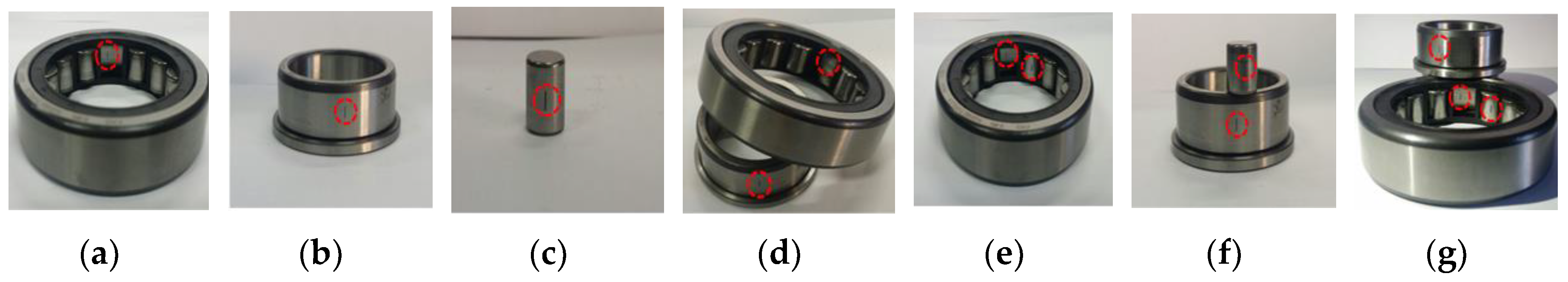
Figure 4.
Block diagram of the proposed method for fault diagnosis in an induction motor.
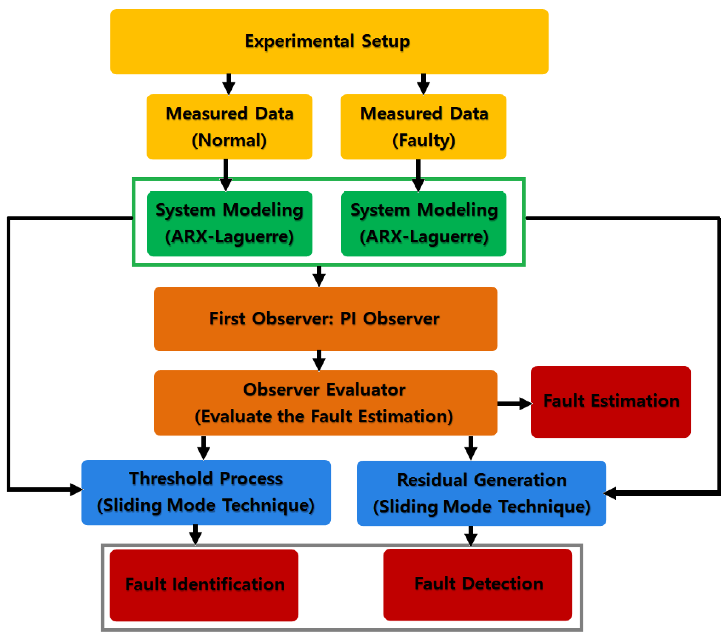
Figure 5.
Block diagram of the sliding mode extended-state ARX-Laguerre PI observer for fault diagnosis in an induction motor.
Figure 5.
Block diagram of the sliding mode extended-state ARX-Laguerre PI observer for fault diagnosis in an induction motor.

Figure 6.
ARX-Laguerre Orthonormal Filter Technique.
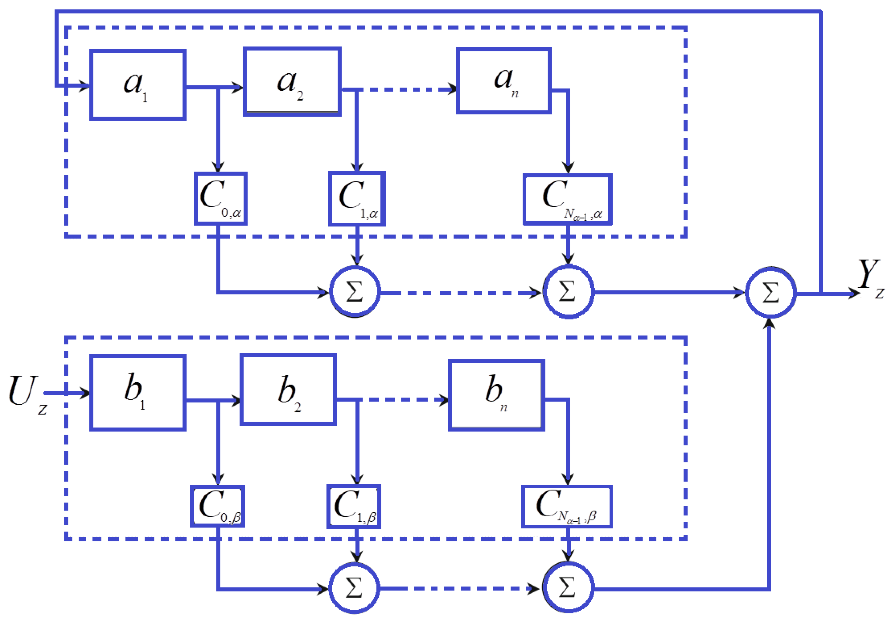
Figure 7.
ARX-Laguerre orthonormal method for system identification/estimation in the normal condition: (a) desired and estimation torque and (b) error.
Figure 7.
ARX-Laguerre orthonormal method for system identification/estimation in the normal condition: (a) desired and estimation torque and (b) error.
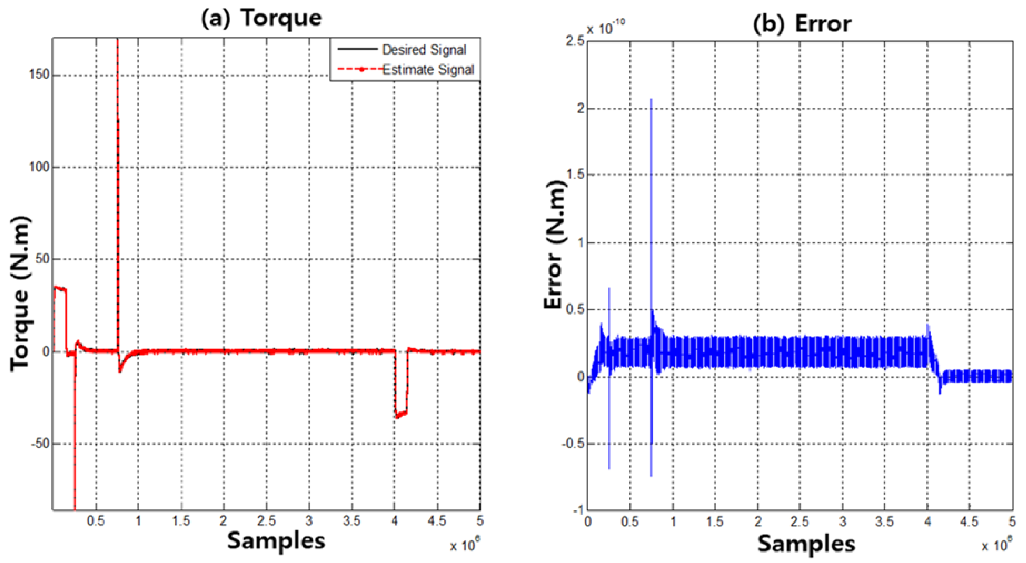
Figure 8.
ARX-Laguerre orthonormal method for system identification/estimation in the faulty condition: (a) desired and estimated torque and (b) error.
Figure 8.
ARX-Laguerre orthonormal method for system identification/estimation in the faulty condition: (a) desired and estimated torque and (b) error.

Figure 9.
Block diagram of the proposed method for fault detection and diagnosis.

Figure 10.
Original raw signals for various faulty conditions.

Figure 11.
Residual signal for the normal condition, faulty condition, and the normal threshold value for fault detection.
Figure 11.
Residual signal for the normal condition, faulty condition, and the normal threshold value for fault detection.

Figure 12.
Residual signal and threshold value for the normal condition for a crack width of 6 mm.

Figure 13.
Ball residual signal, normal threshold signal, and ball threshold signal for the ball faulty condition with a crack width of 6 mm.
Figure 13.
Ball residual signal, normal threshold signal, and ball threshold signal for the ball faulty condition with a crack width of 6 mm.

Figure 14.
Inner residual signal, normal threshold, ball threshold, and inner threshold signal for the inner faulty condition with a crack width of 6 mm.
Figure 14.
Inner residual signal, normal threshold, ball threshold, and inner threshold signal for the inner faulty condition with a crack width of 6 mm.

Figure 15.
Outer residual signal, normal threshold, ball threshold, inner threshold, and outer threshold signal for the outer faulty condition with a crack width of 6 mm.
Figure 15.
Outer residual signal, normal threshold, ball threshold, inner threshold, and outer threshold signal for the outer faulty condition with a crack width of 6 mm.
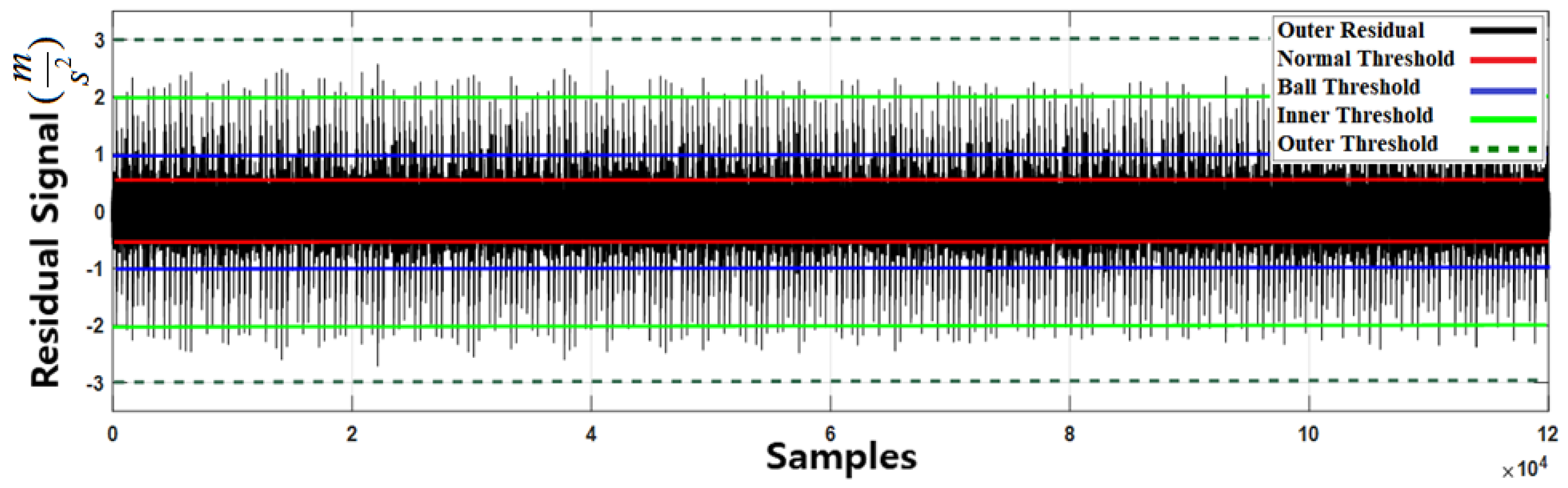
Figure 16.
Residual signal for the inner-ball faulty condition, normal, ball, inner, outer, and inner-ball thresholds with a crack width of 6 mm.
Figure 16.
Residual signal for the inner-ball faulty condition, normal, ball, inner, outer, and inner-ball thresholds with a crack width of 6 mm.
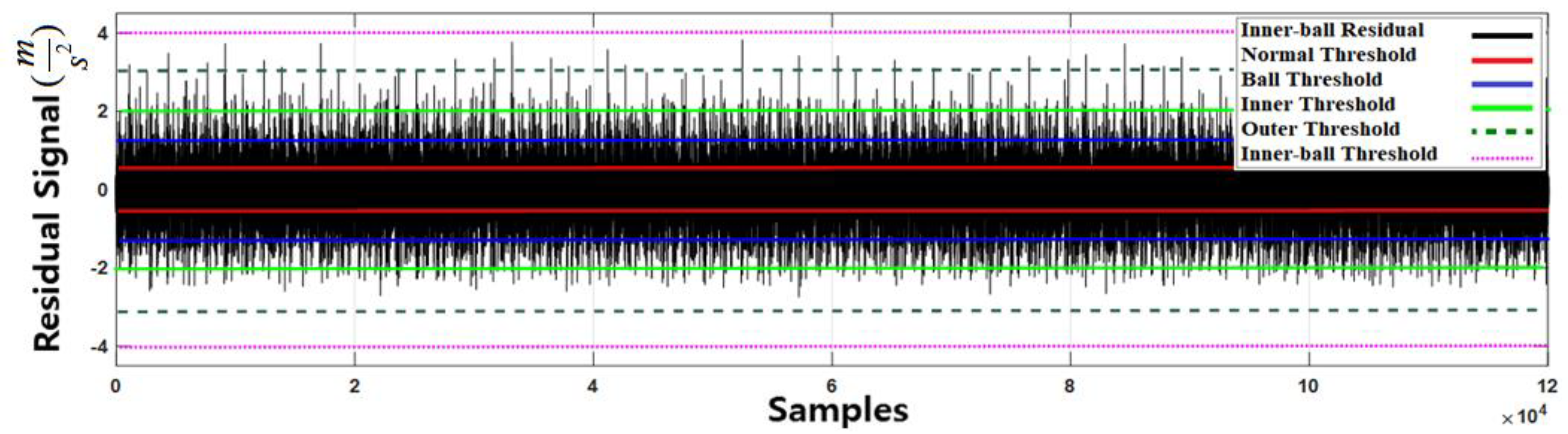
Figure 17.
Residual signal for the outer-ball faulty condition, normal, ball, inner, outer, inner-ball, and outer-ball thresholds with a crack width of 6 mm.
Figure 17.
Residual signal for the outer-ball faulty condition, normal, ball, inner, outer, inner-ball, and outer-ball thresholds with a crack width of 6 mm.

Figure 18.
Residual signal for the inner-outer faulty condition, normal, ball, inner, outer, inner-ball, outer-ball, and inner-outer thresholds with a crack width of 6 mm.
Figure 18.
Residual signal for the inner-outer faulty condition, normal, ball, inner, outer, inner-ball, outer-ball, and inner-outer thresholds with a crack width of 6 mm.

Figure 19.
Residual signal for the inner-outer-ball faulty condition, normal, ball, inner, outer, inner-ball, outer-ball, and inner-outer thresholds with a crack width of 6 mm.
Figure 19.
Residual signal for the inner-outer-ball faulty condition, normal, ball, inner, outer, inner-ball, outer-ball, and inner-outer thresholds with a crack width of 6 mm.

Table 1.
Detailed information of the datasets.
| Dataset | Fault Types | Rotational Speed (RPM) | Fault Crack Size (mm) |
|---|---|---|---|
| Dataset 1 | Normal States | 300 | 3 and 6 |
| IR Fault | 300 | ||
| OR Fault | 300 | ||
| Ball Fault | 300 | ||
| Inner-Outer Fault | 300 | ||
| Inner-Ball Fault | 300 | ||
| Outer-Ball Fault | 300 | ||
| Inner-Outer-Ball Fault | 300 | ||
| Dataset 2 | Normal States | 400 | 3 and 6 |
| IR Fault | 400 | ||
| OR Fault | 400 | ||
| Ball Fault | 400 | ||
| Inner-Outer Fault | 400 | ||
| Inner-Ball Fault | 400 | ||
| Outer-Ball Fault | 400 | ||
| Inner-Outer-Ball Fault | 400 | ||
| Dataset 3 | Normal States | 450 | 3 and 6 |
| IR Fault | 450 | ||
| OR Fault | 450 | ||
| Ball Fault | 450 | ||
| Inner-Outer Fault | 450 | ||
| Inner-Ball Fault | 450 | ||
| Outer-Ball Fault | 450 | ||
| Inner-Outer-Ball Fault | 450 | ||
| Dataset 4 | Normal States | 500 | 3 and 6 |
| IR Fault | 500 | ||
| OR Fault | 500 | ||
| Ball Fault | 500 | ||
| Inner-Outer Fault | 500 | ||
| Inner-Ball Fault | 500 | ||
| Outer-Ball Fault | 500 | ||
| Inner-Outer-Ball Fault | 500 |
Table 2.
Fault diagnosis results using dataset 1 with the proposed method and ARX-Laguerre proportional integral observation (ALPIO) when the torque speed is 300 RPM.
Table 2.
Fault diagnosis results using dataset 1 with the proposed method and ARX-Laguerre proportional integral observation (ALPIO) when the torque speed is 300 RPM.
| Algorithms | Proposed Method | ALPIO | ||
|---|---|---|---|---|
| Crack Diameters (mm) | 3 | 6 | 3 | 6 |
| Normal Stat | 100% | 100% | 80% | 80% |
| IR Fault | 95% | 96% | 67% | 73% |
| OR Fault | 95% | 97% | 72% | 80% |
| Ball Fault | 96% | 100% | 78% | 74% |
| IR-Ball Fault | 93% | 98% | 80% | 81% |
| OR-Ball Fault | 97% | 97% | 82% | 82% |
| IR-OR Fault | 98% | 98% | 78% | 82% |
| IR-OR-Ball Fault | 97% | 97% | 78% | 81% |
| Average | 96.1% | 97.9% | 77.6% | 79.4% |
Table 3.
Fault diagnosis results using dataset 2 with the proposed method and ARX-Laguerre proportional integral observation (ALPIO) when the torque speed is 400 RPM.
Table 3.
Fault diagnosis results using dataset 2 with the proposed method and ARX-Laguerre proportional integral observation (ALPIO) when the torque speed is 400 RPM.
| Algorithms | Proposed Method | ALPIO | ||
|---|---|---|---|---|
| Crack Diameters (mm) | 3 | 6 | 3 | 6 |
| Normal Stat | 100% | 100% | 86% | 86% |
| IR Fault | 95% | 96% | 70% | 73% |
| OR Fault | 96% | 97% | 72% | 82% |
| Ball Fault | 97% | 99% | 78% | 79% |
| IR-Ball Fault | 94% | 98% | 80% | 84% |
| OR-Ball Fault | 97% | 97% | 83% | 83% |
| IR-OR Fault | 98% | 100% | 78% | 82% |
| IR-OR-Ball Fault | 97% | 98% | 79% | 80% |
| Average | 96.8% | 98.2% | 78.3% | 81.1% |
Table 4.
Fault diagnosis results using dataset 3 with the proposed method and ARX-Laguerre proportional integral observation (ALPIO) when the torque speed is 450 RPM.
Table 4.
Fault diagnosis results using dataset 3 with the proposed method and ARX-Laguerre proportional integral observation (ALPIO) when the torque speed is 450 RPM.
| Algorithms | Proposed Method | ALPIO | ||
|---|---|---|---|---|
| Crack Diameters (mm) | 3 | 6 | 3 | 6 |
| Normal Stat | 100% | 100% | 88% | 88% |
| IR Fault | 97% | 97% | 75% | 78% |
| OR Fault | 97% | 98% | 76% | 82% |
| Ball Fault | 97% | 99% | 82% | 82% |
| IR-Ball Fault | 95% | 98% | 83% | 84% |
| OR-Ball Fault | 97% | 98% | 84% | 84% |
| IR-OR Fault | 98% | 99% | 80% | 82% |
| IR-OR-Ball Fault | 97% | 97% | 79% | 81% |
| Average | 97.3% | 98.8% | 79.6% | 82.4% |
Table 5.
Fault diagnosis results of dataset 4 using the proposed method and ARX-Laguerre proportional integral observation (ALPIO) when the torque speed is 500 RPM.
Table 5.
Fault diagnosis results of dataset 4 using the proposed method and ARX-Laguerre proportional integral observation (ALPIO) when the torque speed is 500 RPM.
| Algorithms | Proposed Method | ALPIO | ||
|---|---|---|---|---|
| Crack Diameters (mm) | 3 | 6 | 3 | 6 |
| Normal Stat | 100% | 100% | 90% | 90% |
| IR Fault | 97% | 97% | 81% | 83% |
| OR Fault | 98% | 98% | 78% | 82% |
| Ball Fault | 97% | 99% | 82% | 84% |
| IR-Ball Fault | 97% | 97% | 83% | 85% |
| OR-Ball Fault | 98% | 99% | 85% | 85% |
| IR-OR Fault | 98% | 99% | 82% | 82% |
| IR-OR-Ball Fault | 97% | 98% | 82% | 83% |
| Average | 99.9% | 99.1% | 81.2% | 84.6% |
Table 6.
Confusion matrix using dataset 2 with the proposed method when the torque speed is 400 RPM and the crack size is 3 mm.
Table 6.
Confusion matrix using dataset 2 with the proposed method when the torque speed is 400 RPM and the crack size is 3 mm.
| Actual Class | |||||||||
|---|---|---|---|---|---|---|---|---|---|
| Predict Class | Normal | Ball | IR | OR | IR-Ball | OR-Ball | IR-OR | IR-OR-Ball | Precision |
| Normal | 100% | 0 | 0 | 0 | 0 | 0 | 0 | 0 | 100% 0% |
| Ball | 1% | 97% | 0 | 0 | 1% | 1% | 0 | 0 | 97% 3% |
| IR | 0 | 1% | 95% | 2% | 1% | 0 | 1% | 0 | 95% 5% |
| OR | 0 | 0 | 1% | 96% | 3% | 0 | 0 | 0 | 96% 4% |
| IR-Ball | 0 | 0 | 0 | 4% | 94% | 1% | 1% | 0 | 94% 6% |
| OR-Ball | 1% | 1% | 0 | 1% | 0 | 97% | 0 | 0 | 97% 3% |
| IR-OR | 1% | 0 | 0 | 0 | 1% | 0 | 98% | 0 | 98% 2% |
| IR-OR-Ball | 0 | 0 | 0 | 0 | 0 | 0 | 3% | 97% | 97% 3% |
| Recall | 97.1% 2.9% | 97.9% 2.1% | 99% 1% | 93.2% 6.8% | 94% 6% | 97.9% 2.1% | 95.1% 4.9% | 100% 0% | 95.07% 4.93% |
Table 7.
Confusion matrix using dataset 2 with the proposed method when the torque speed is 400 RPM and the crack size is 6 mm.
Table 7.
Confusion matrix using dataset 2 with the proposed method when the torque speed is 400 RPM and the crack size is 6 mm.
| Actual Class | |||||||||
|---|---|---|---|---|---|---|---|---|---|
| Predict Class | Normal | Ball | IR | OR | IR-Ball | OR-Ball | IR-OR | IR-OR-Ball | Precision |
| Normal | 100% | 0 | 0 | 0 | 0 | 0 | 0 | 0 | 100% 0% |
| Ball | 0 | 99% | 0 | 1% | 0 | 0 | 0 | 0 | 99% 1% |
| IR | 0 | 0 | 96% | 3% | 0 | 0 | 1% | 0 | 96% 4% |
| OR | 0 | 0 | 2% | 97% | 1% | 0 | 0 | 0 | 97% 3% |
| IR-Ball | 0 | 2% | 0 | 0 | 98% | 0 | 0 | 0 | 98% 2% |
| OR-Ball | 1% | 2% | 0 | 0 | 0 | 97% | 0 | 0 | 97% 3% |
| IR-OR | 0 | 0 | 0 | 0 | 0 | 0 | 100% | 0 | 100% 0% |
| IR-OR-Ball | 0 | 0 | 1% | 0 | 0 | 0 | 1% | 98% | 98% 2% |
| Recall | 99% 1% | 96.1% 3.9% | 97% 3% | 96% 4% | 99% 1% | 100% 0% | 98% 2% | 100% 0% | 98.13% 1.87% |
Table 8.
Fault diagnosis results for various motor speeds using the proposed method and ALPIO (crack size = 3 mm).
Table 8.
Fault diagnosis results for various motor speeds using the proposed method and ALPIO (crack size = 3 mm).
| Algorithms | Proposed Method | ALPIO | ||||||
|---|---|---|---|---|---|---|---|---|
| Motor Speed (RPM) | 300 | 400 | 450 | 500 | 300 | 400 | 450 | 500 |
| Normal Stat | 100% | 100% | 100% | 100% | 80% | 86% | 88% | 90% |
| IR Fault | 95% | 95% | 97% | 97% | 67% | 70% | 75% | 83% |
| OR Fault | 95% | 96% | 97% | 98% | 72% | 72% | 76% | 82% |
| Ball Fault | 96% | 97% | 97% | 97% | 77% | 78% | 82% | 84% |
| IR-Ball Fault | 93% | 94% | 95% | 97% | 80% | 80% | 83% | 85% |
| OR-Ball Fault | 97% | 97% | 97% | 98% | 79% | 83% | 84% | 80% |
| IR-OR Fault | 98% | 98% | 98% | 98% | 78% | 82% | 72% | 82% |
| IR-OR-Ball Fault | 97% | 97% | 97% | 98% | 79% | 76% | 79% | 83% |
| Average | 96.4% | 96.8% | 97.2% | 97.9% | 76.5% | 78.4% | 79.9% | 83.6% |
Table 9.
Fault diagnosis results for various motor speeds using the proposed method and ALPIO (crack size=6 mm).
Table 9.
Fault diagnosis results for various motor speeds using the proposed method and ALPIO (crack size=6 mm).
| Algorithms | Proposed Method | ALPIO | ||||||
|---|---|---|---|---|---|---|---|---|
| Motor Speed (RPM) | 300 | 400 | 450 | 500 | 300 | 400 | 450 | 500 |
| Normal Stat | 100% | 100% | 100% | 100% | 80% | 86% | 88% | 90% |
| IR Fault | 96% | 96% | 97% | 97% | 73% | 73% | 78% | 83% |
| OR Fault | 97% | 97% | 98% | 98% | 80% | 76% | 82% | 82% |
| Ball Fault | 100% | 99% | 99% | 99% | 74% | 78% | 82% | 84% |
| IR-Ball Fault | 98% | 98% | 98% | 97% | 81% | 84% | 84% | 85% |
| OR-Ball Fault | 97% | 97% | 98% | 99% | 82% | 83% | 84% | 85% |
| IR-OR Fault | 98% | 100% | 99% | 99% | 82% | 82% | 79% | 82% |
| IR-OR-Ball Fault | 97% | 98% | 97% | 98% | 78% | 80% | 82% | 83% |
| Average | 97.9% | 98.1% | 98.2% | 98.4% | 78.8% | 80.2% | 82.4% | 84.3% |
© 2019 by the authors. Licensee MDPI, Basel, Switzerland. This article is an open access article distributed under the terms and conditions of the Creative Commons Attribution (CC BY) license (http://creativecommons.org/licenses/by/4.0/).
Share and Cite
MDPI and ACS Style
Piltan, F.; Kim, J.-M. Nonlinear Extended-state ARX-Laguerre PI Observer Fault Diagnosis of Bearings. Appl. Sci. 2019, 9, 888. https://doi.org/10.3390/app9050888
AMA Style
Piltan F, Kim J-M. Nonlinear Extended-state ARX-Laguerre PI Observer Fault Diagnosis of Bearings. Applied Sciences. 2019; 9(5):888. https://doi.org/10.3390/app9050888
Chicago/Turabian StylePiltan, Farzin, and Jong-Myon Kim. 2019. "Nonlinear Extended-state ARX-Laguerre PI Observer Fault Diagnosis of Bearings" Applied Sciences 9, no. 5: 888. https://doi.org/10.3390/app9050888
Note that from the first issue of 2016, this journal uses article numbers instead of page numbers. See further details here.