Fast Cylinder Shape Matching Using Random Sample Consensus in Large Scale Point Cloud


Culture Technology Research Institute, Chung-Ang University, Seoul 06974, Korea
*
Author to whom correspondence should be addressed.
Appl. Sci. 2019, 9(5), 974; https://doi.org/10.3390/app9050974
Submission received: 31 January 2019
/
Revised: 3 March 2019
/
Accepted: 4 March 2019
/
Published: 7 March 2019
(This article belongs to the Special Issue Machine Learning and Compressed Sensing in Image Reconstruction)
Abstract
:In this paper, an algorithm is proposed that can perform cylinder type matching faster than the existing method in point clouds that represent space. The existing matching method uses Hough transform and completes the matching through preprocessing such as noise filtering, normal estimation, and segmentation. The proposed method completes the matching through the methodology of random sample consensus (RANSAC) and principal component analysis (PCA). Cylindrical pipe estimation is based on two mathematical models that compute the parameters and combine the results to predict spheres and lines. RANSAC fitting computes the center and radius of the sphere, which can be the radius of the cylinder axis and finds straight and curved areas through PCA. This allows fast matching without normal estimation and segmentation. Linear and curved regions are distinguished by a discriminant using eigenvalues. The linear region is the sum of the vectors of linear candidates, and the curved region is matched by a Catmull–Rom spline. The proposed method is expected to improve the work efficiency of the reverse design by matching linear and curved cylinder estimation without vertical/horizontal constraint and segmentation. It is also more than 10 times faster while maintaining the accuracy of the conventional method.
Keywords:
point cloud; RANSAC; Catmull-Rom; pipe estimation; PCA; Lidar; spline; detection; iterative method; random sample1. Introduction
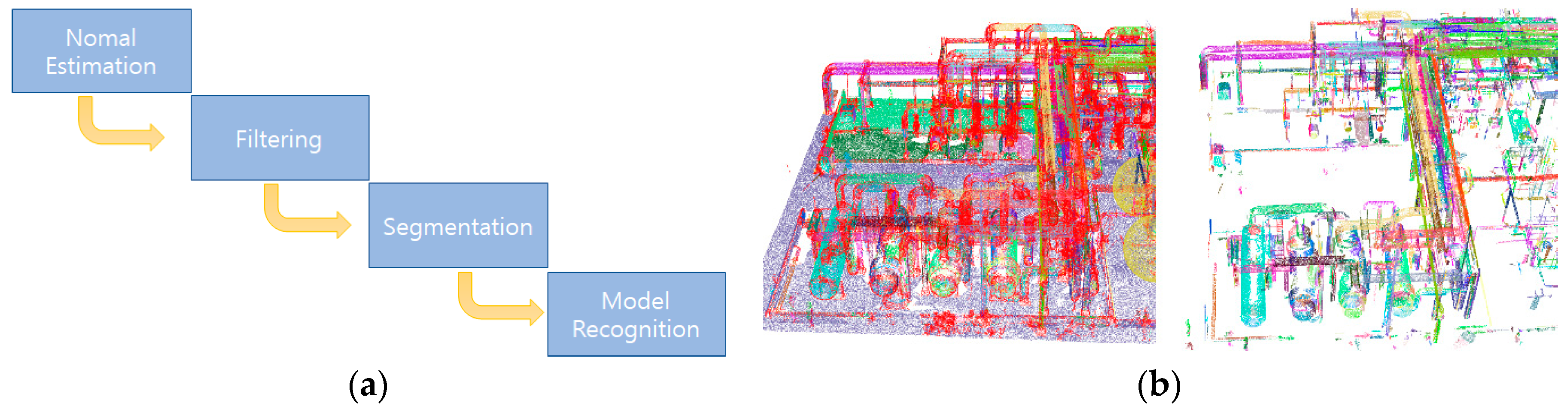
A variety of studies have been conducted in the computer vision field to recognize objects in 3D space. For example, researchers have studied depth information through a camera (stereo matching) or an infrared camera that imitates an eye as well as object recognition and movement by measuring depth through a laser scanner. Among them, measurement using a space scanner is relatively more precise than measurement using a camera; thus, it is widely used to construct point clouds. The 3D scanner emits an infrared laser into space and calculates the distance by measuring the time it takes for the object to be reflected back. The light has several characteristics in a specific time and space. Among these, maintaining straightness and consistent velocity enables a relatively accurate distance measurement. Point clouds obtained from 3D scanners are generally sufficient for human perception but are not recognized by computers. Therefore, the computer is subjected to various preprocessing steps, such as normal estimation, segmentation, and filtering, to recognize objects in the point cloud (shown in Figure 1).
The normal estimate is obtained by constructing a covariance matrix from the surrounding points using the k-d tree data structure and calculating the eigenvectors. When the normal estimation is completed, it is divided into a set of points with a common normal that meet certain criteria. The divided sets undergo postprocessing to determine what kind of object each set is.
In recent years, plant construction has been based on 3D design, so it is easy to check the structure interference or make modifications/changes, and it is possible to efficiently design and to train in areas such as fire, disaster, and operation using virtual technology. On the other hand, it is more efficient to maintain/repair through reverse design because the existing plant site is huge, and reconstruction is impossible. Reverse design is aimed at obtaining meaningful data through digitization in three dimensions for constructed facilities or facilities under construction. Therefore, the demand for reverse design is increasing.
This paper describes a method for quickly recognizing cylinder-shaped objects that take up a large portion of plant facilities. A plant facility of large scale entails a large opportunity cost for 3D scanning and consists of a very large set of points. Therefore, since matching requires a lot of computer resources (CPU, memory, db, power usage), time, and manpower, relatively fast and accurate matching is the only way to reduce costs. In general, cylinder-shaped objects are matched using region growing, Hough transform, random sample consensus (RANSAC), and machine learning.
Region growing is a process for segmentation and is classified into a set of normals that maintain similar directionality in a point cloud. Hough transform is a method of estimating the direction of a cylinder ultimately by replacing the normal formed by segmented data with a Hough space [2]. Both of these methods result in an exponential increase in processing time and memory usage as the numbers of data points increase. On the other hand, primitive fitting using RANSAC is relatively fast, but gives inaccurate results due to noise and curved areas. To overcome this drawback, this paper uses RANSAC, estimates the direction of the cylinder through sphere fitting, and computes the cylinder length through principal component analysis (PCA). The proposed method is robust against noise and shows fast matching results while maintaining relative accuracy.
Because the plant is large (the Ulsan Petrochemical Complex site in Korea has 29,916,000 square meters), it takes a significant amount of opportunity cost to handle reverse engineering manually. In addition, since many computer resources are used for reverse design, appropriate filtering and data structure must be used so that it can be processed without overflow. Therefore, complete automation is virtually impossible. This paper is meaningful in terms of reducing the opportunity cost of manual operation rather than perfecting automation and operating computer resources efficiently.
2. Related Research
In general, to estimate an object, a mathematical primitive (parametric shape) is used and accessed through RANSAC [3], Hough transform, or a machine learning algorithm.
Abusaina estimated spherical structures using Hough transform. In order to speed up the computation, the authors proposed a method to increase speed and maintain accuracy by partially performing the calculation without searching the entire point cloud [4]. Zhang estimated the roof through RANSAC. The authors proposed a multi model fitting method by applying Bayes’ rule and a PCA algorithm to extend plane fit [5]. Garcia proposed a mathematical definition of various basic shapes to be applied to RANSAC and a primitive shape decomposition algorithm for estimating objects containing basic shapes in order to apply basic shape fitting to robot grasping [6]. Su used Hough transform to estimate cylinder shape. Cylinder estimation requires a 5D Hough transform, which is computationally inefficient and generally computed separately in 2D and 3D. The authors proposed a multiple cylinder detection method using a coarse-to-fine approach and a clustering algorithm [7]. Jones proposed a method of evaluating 3D point cloud histograms through support vector machine (SVM), which is the most similar to the model in the database [8]. Liu first extracted and removed the data vertically and horizontally from the ground, called T1 and T2. After that, Hough transform was used to project a plane on the normal vector and propose a cylinder shape estimation method through circle fitting [9,10,11]. Son determined the central axis of the pipe by the skeleton extraction algorithm through Laplacian smoothing and estimated the curved region and the T shape of the cylinder by dividing [12]. Huang classified meaningful data through fast point feature histogram (FPFH) and SVM and segmented it with the classical flood-fill algorithm. Matching was completed through RANSAC in the segmented data. However, the proposed method found only relatively complex shapes such as ball valves and flanges, because those have unique feature points. In other words, a unique feature point is needed for histogram comparisons [13]. Pang extracted primitive models using FPFH in point clouds and recognized objects through Adaboost with library models. The recognition object is merged/adjusted based on directionality and start/end position, and the automatic modeling is completed. However, it takes more than 30 minutes for 10 million pieces of data [14]. Rongqi computed one plane of normals on the Gaussian sphere after normal estimation through RANSAC. Projection of segmented points on the plane estimates the radius and length of the cylinder. If there is an intersection point with another cylinder through the estimated starting and ending points of the cylinder, it is judged as an elbow. Experimental results show relatively accurate results, but it required a lot of execution time [15].
In the existing study, SVM and the method using RANSAC could extract the cylinder shape, but the center axis and the radius could not be confirmed. To solve this problem, the Hough transform was used. The Hough transform is excellent in terms of accuracy but requires a large amount of computation and a segmentation process. In addition, it has the disadvantage of requiring a lot of resources compared with RANSAC. Partitioning is a method of gradually searching for neighboring points and sorting out a group that meets certain criteria. As the point cloud grows, the execution time increases. Therefore, in a point cloud with a large number of points, object estimation requires a relatively large opportunity cost. In order to overcome these disadvantages, constraints are used to filter the data through vertical/horizontal conditions with the ground. Therefore, data filtering using constraints is inevitable in matching pipes with oblique lines.
In this paper, a linear axis/curved region estimation method of constructing a central axis candidate group by fitting RANSAC without constraint, normal estimation, and segmentation is proposed.
3. Center Axis Estimation
In this paper, RANSAC is used to estimate cylindrical objects in a point cloud. RANSAC is a methodology [16,17] that analyzes all the data by repeatedly sampling from the given data. Because it uses only some data, it shows relatively fast and strong noise. It also consumes fewer resources than Hough transform and is therefore worth using. RANSAC fitting requires defining a mathematical model of sphere and line. By specifying the parameters that fit the model of the defined sphere, the center axis candidate (center point and radius) can be constructed. The central axis candidates are also in the point cloud. The center axis of the pipe is estimated from the center axis candidate group through the length of the region corresponding to the straight line model and the radius average.
3.1. Sphere Modeling
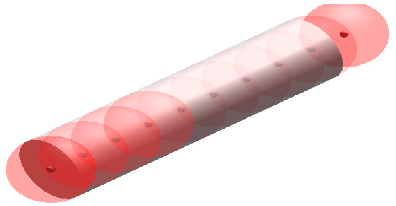
The spheres present the points that can estimate the center axis and radius of the cylinder. Figure 2 shows a sphere with the same diameter as the cylinder moving along the inside of the cylinder, leaving a trace of the center point. In the point cloud, a center point and a radius can be calculated, as shown in Figure 2, if it performs spherical fitting through neighboring points around a point.
The mathematical model of the sphere is shown in Equation (1) and the parameters a, b, c, and r are determined through RANSAC to calculate the radius and center of the sphere.
Equation (1) becomes the determinant Equation (2) and parameters can be determined through the pseudo-inverse of Equation (3).
3.2. Straight Line Modeling
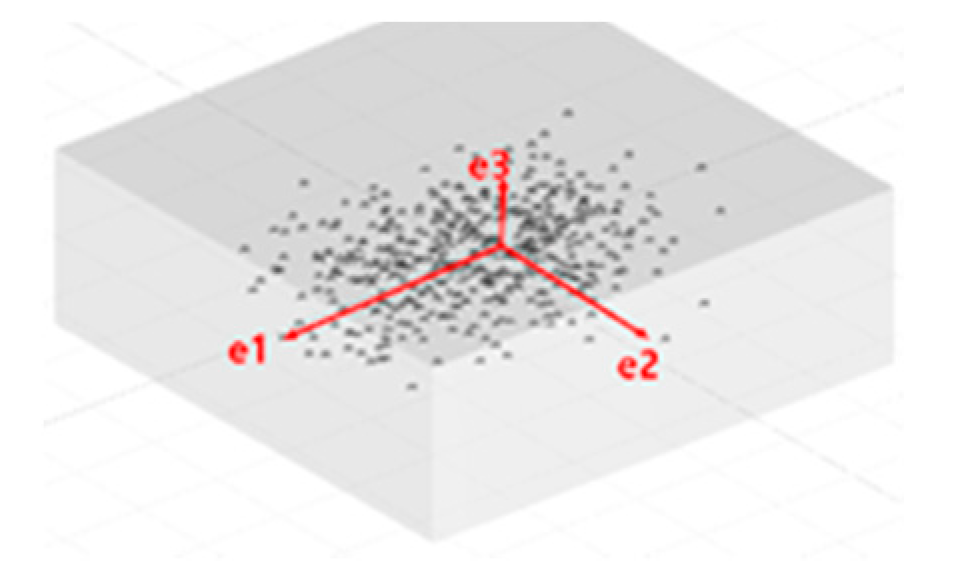
As shown in Section 3.1, directionality can be estimated through the set of trajectories using spheres, which can be assumed to be the center axis of the cylinder. Therefore, the central axis estimation models the straight line and uses principal component analysis (PCA). PCA is a statistical approach [18,19] that estimates the direction of e2, e3, etc., which are perpendicular to e1 and e1 with the largest variance of data, as shown in Figure 3. Therefore, if e1 is found, the direction of the cylinder’s center axis can be known.
PCA constructs a covariance matrix as shown in Equations (4) and (5), and eigen-decomposition of the covariance matrix yields a direction vector.
The eigenvalue decomposition can be used to find a nonzero vector and an eigenvalue that can hold. Here, a way to determine if the given data is meaningful (straight/curved) is presented.
Equation (6) means the ratio of the eigenvalue . If is close to 0 ( ), it is a straight line, and if it is within a certain range (), it is a curve. Using a discriminant based on neighboring points at one point can reduce execution time.
3.3. Matching and Filtering
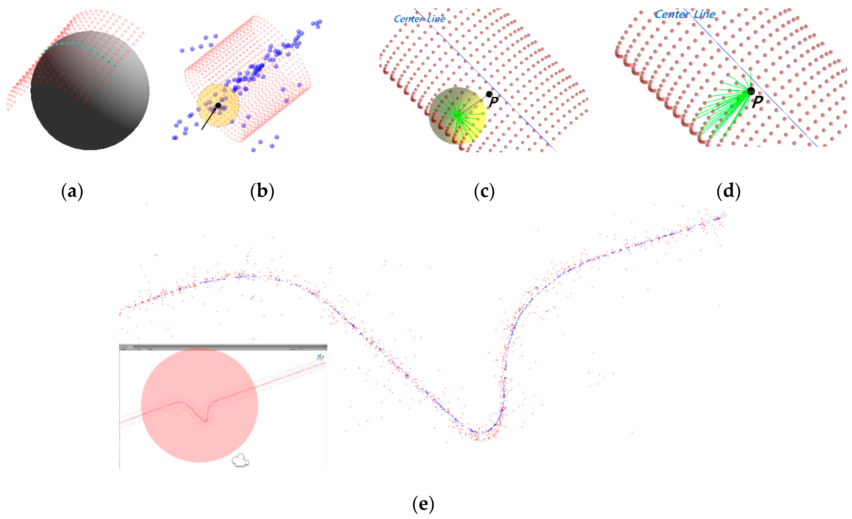
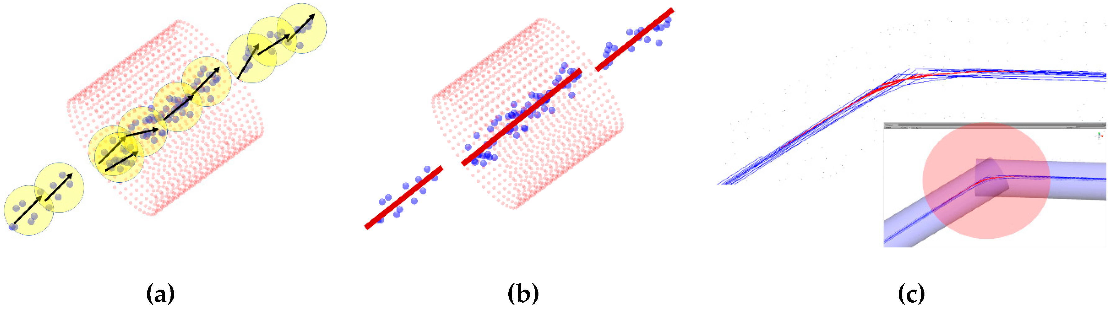
The estimation of the center axis of the cylinder is obtained by matching the candidate group matching the straight line in the set of the center point and the radius obtained repeatedly through the spherical fit described in Section 3.1. Figure 4a depicts the center and radius estimates through spherical fitting, where k is the number of neighboring points to a point in the point cloud and RANSAC fitting is applied to four of these points to obtain the center point and radius. In this paper, the fitting is performed twice at one point, in order to increase the hit ratio. As shown in Figure 4c, first it performs the sphere fitting to six points in nine neighboring points based on one point once. In the result, if 36 neighboring points are searched again in P, the probability of selecting a neighboring point forming a cylinder cross-section at a point inside the cylinder can be increased, as shown in Figure 4d. Repeatedly, it is possible to obtain a central axis candidate set with higher accuracy than a single RANSAC fitting.
Since the center axis candidates thus obtained have many outliers, the outliers are removed by filtering. Filter processing simply means local averaging, and is shown in Figure 4b. Local average (blue points of Figure 4e) can be obtained by repeatedly calculating the average coordinates of the neighboring points of each point in the center axis candidate set (red points) of Figure 4e. In the filtered center axis candidates (blue points), the central axis estimation can be obtained through the eigenvectors shown in Section 3.2.
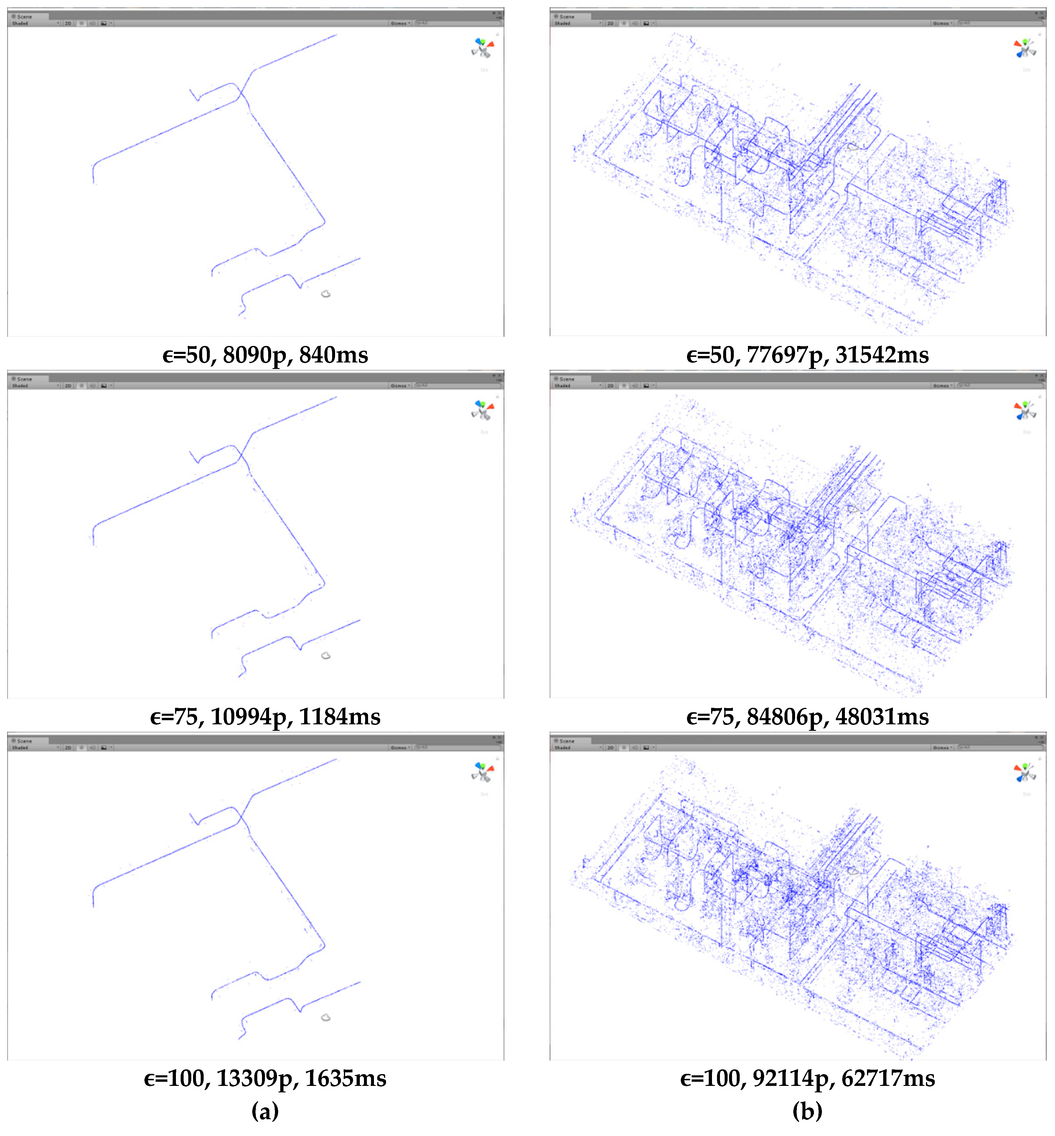
In principle, matching is targeted to all point clouds, but is performed on arbitrary data to reduce execution time. This is because the number of points forming the circumference of the cylinder is large, so a similar result can be obtained by matching at a constant interval/ratio. Figure 5 shows the execution time as the matching ratio increases.
Figure 5a shows that the execution time and matching results linearly increase when the value of increases from 1 to 100 with already segmented data. If it is above a certain level (50%), the center axis estimation result is sufficient to match the cylinder, so it is better to select the appropriate value. Figure 5b shows that the execution time linearly increases as the value of increases when the data is not segmented, but the center axis estimation result is relatively slowed at around 45% (red circle A). Noise also appears to increase. Therefore, the appropriate value should be selected for fast and accurate matching. As a result, if the total number or density of point clouds is high, execution time can be reduced while maintaining relative accuracy through the appropriate .
When the center axis estimation is completed through the appropriate value, the accuracy of the matching cylinder can be confirmed by checking its diameter, as shown in Figure 6. Figure 6a shows the distance between two points with CloudCompare, and Figure 6b shows the result of matching with the proposed method. In Figure 6a, the distance between two points is 0.54 m, and in Figure 6b, scale X and Z of the cylinder is 0.53 m and the diameters are almost equal (1 cm error). The actual cylinder diameter is 20 inches (0.508 m) and there is some error (2 cm).
3.4. Center Axis Estimation
Figure 7 depicts the central axis estimation. Figure 7a is the result of calculating the eigenvectors based on the neighboring points at one point, and Figure 7b is the result of estimating the direction and length through the sum of the eigenvectors satisfying a certain criterion. Here, the criterion is the distance and angle between two vectors. That is, if the angle formed by two vectors and the distance are within a certain range, the two vectors are one vector. At this time, the radius average of a set of points constituting one vector is the radius of the cylinder. Figure 7c is the result of matching the straight line through the sum of the eigenvectors (blue lines).
4. Curve(elbow) Estimation
In order to express a smooth curve, a method of creating the shape of a curve is defined in a graphics field by defining a control point. Typical examples are Bezier, B-spline, Non-uniform rational B-spline(NURBS), and cubic spline. At this time, it is divided into an interpolation method and an approximation method depending on whether or not the curve passes through the control point. As shown in Section 3, since the estimated center axis is a set of points, the tangent of the curve in all sections through the directionality of the points can be estimated. PCA, which can identify directionality through the distribution of point sets, is a method of compressing into low-dimensional data by mapping to statistically distributed axes [18]. This makes it possible to construct directionality in all sections. The directionality of neighboring points can play an important role in computing the control points of the spline curve. Since the control points are composed of tangent lines of curves, this paper constructs the spline through the control points and uses the Catmull–Rom spline algorithm.
4.1. Spline Curve
The spline curve is a smooth curve that passes through a number of control points and interpolates between them with a reference polynomial [20]. The control point estimate for the spline curve is constructed as shown in Figure 8.
Figure 8a depicts the method of estimating the tangent of the curve whose eigenvalue is the largest in the center point data of a certain region through PCA. Figure 8b describes the control point estimation through the intersections of tangents by performing the process in Figure 8a at several points. Using Figure 8b, the matching is completed as shown in Figure 8c. Since the control point is estimated in the linear region as shown in Figure 8, the estimated control point is again verified by the discriminant equation. PCA is decomposed into a direction (eigenvector) and a magnitude (eigenvalue). In the discriminant of Equation (6) shown in Section 3.2, it is judged whether the control point has the tendency of a straight line or a curve.
4.2. Catmull-Rom Spline
The Catmull–Rom spline is a form of cubic interpolation spline formed by tangents at each point that can form a curve through a given control point and can be defined by the basis function [21] of Equation (7). A basic function is a basic element that can express a continuous function through a linear combination in a function space.
The slope of the curve is changed, as shown in Figure 9, by the value of in Equation (7).
Curves by Catmull–Rom splines should have control points in order. In the case of four control points, Figure 10a shows the points in order and Figure 10b shows the points without order. Therefore, the order of the control points must be determined for the curve configuration.
To determine the order of the control points, they are projected in the direction with the largest eigenvalue. Figure 10c shows the control points projected on the direction vector with the largest variance. By aligning the sizes of the orthogonal vectors in ascending order, aligned control points for the estimation curve can be obtained. The finally aligned control points are traces of the bent cylinder.
5. Experiments and Discussions
Verification of the proposed method proceeded through segmented and nonsegmented data. The system used in the experiment has Intel 8250U 3.4 G CPU, 8 G memory, and uses Unity3D. The experiment used the following pseudo-code (shown in Scheme 1):
Code a is the center axis estimation, where DCL is the matching result, DFLT is the filtered matching result, and is the PCA result. Code b constructs the cylinder candidate group (DEST) when the distance and angle are within a certain range in and finally obtains the cylinder (DCYL). Code c finds the intersection point (DCP) of the surrounding tangents when is a curve and completes the spline (DSPL) through the discriminant.
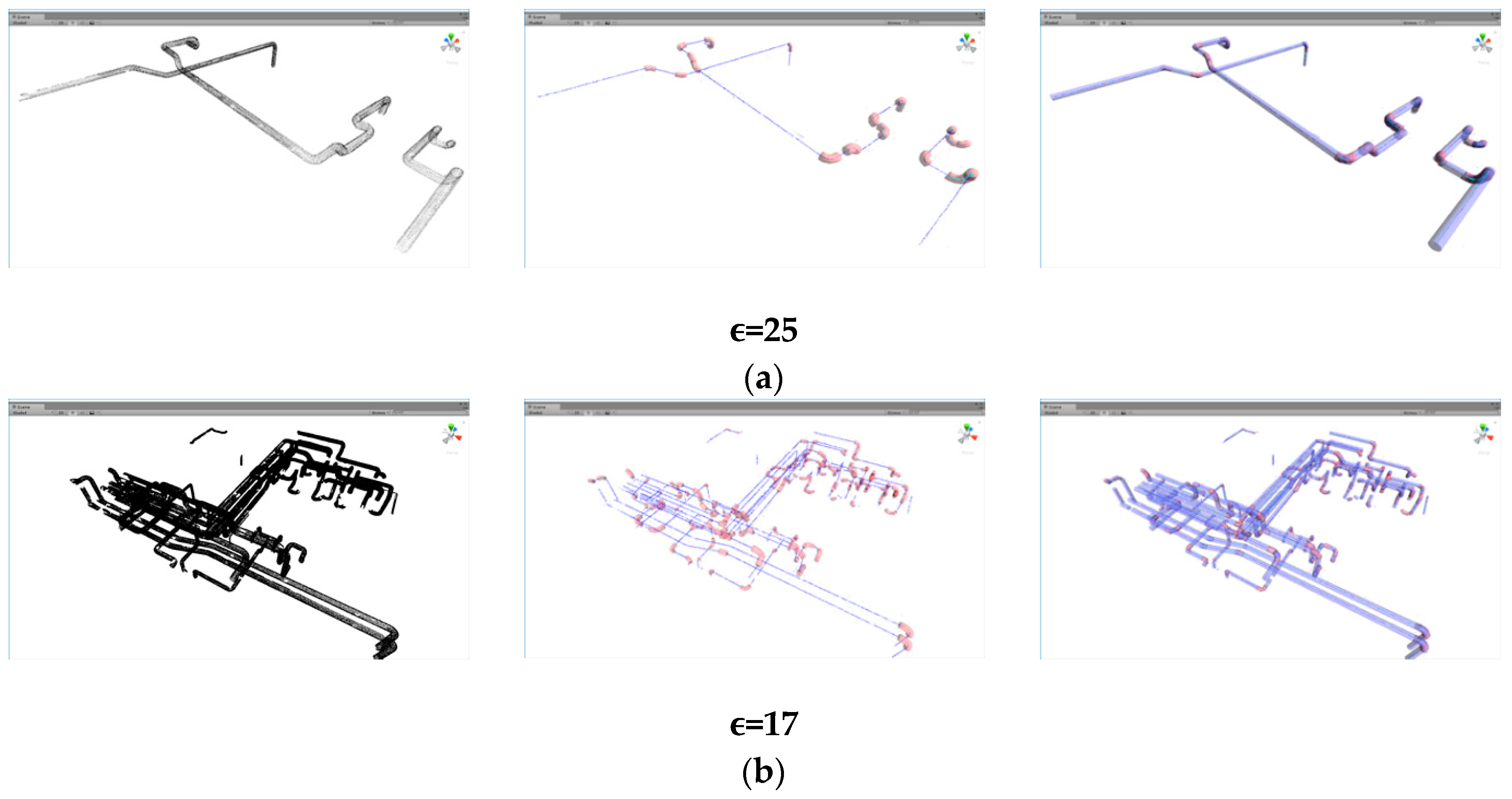
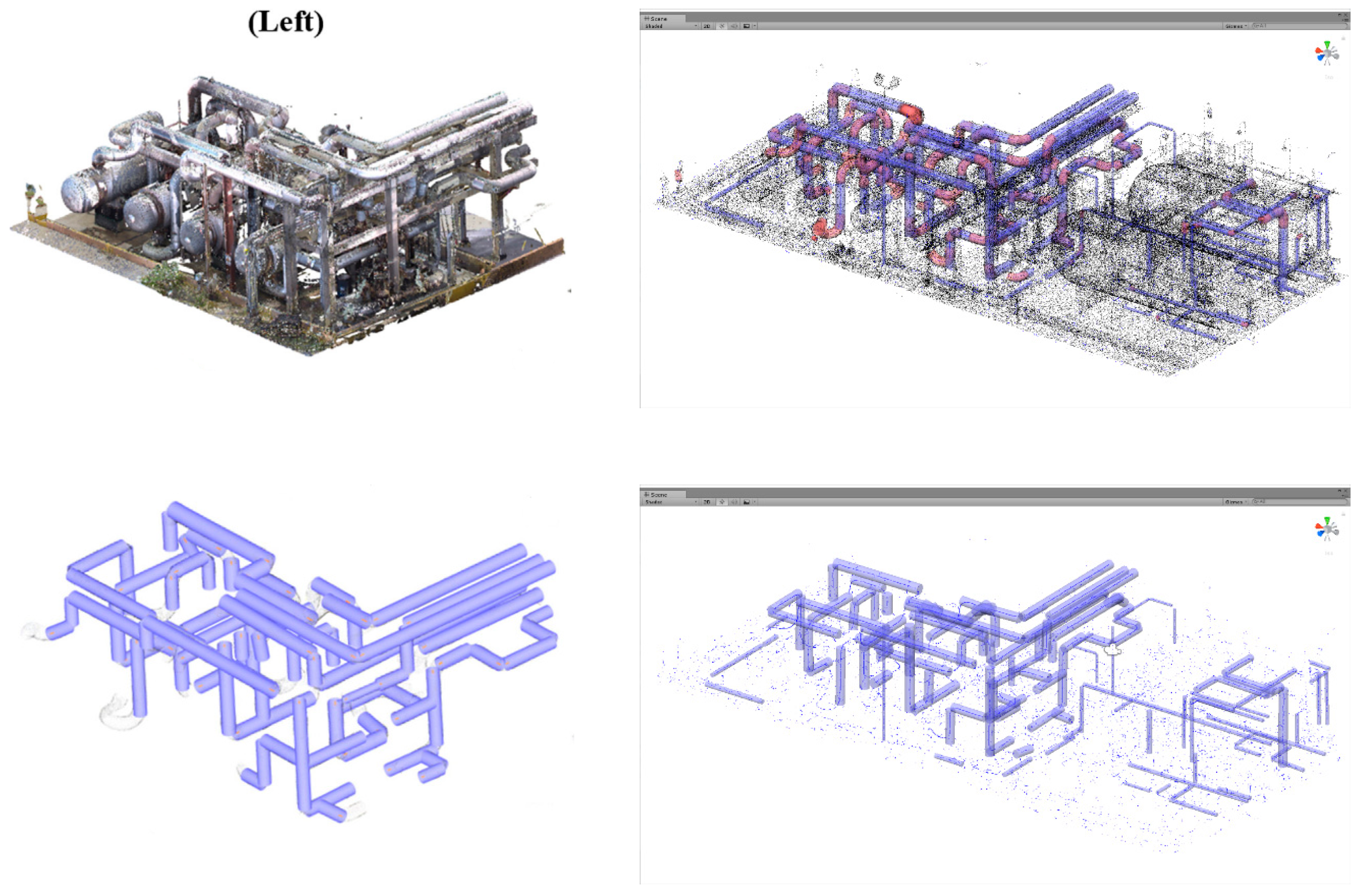
Figure 11a shows segmented data consisting of 20,107 points. From left to right, the process is: place point clouds in order, map the curved region to the center axis estimation result, map the straight and curved regions. The figure shows results that include most of the curved regions that exist.
Figure 11b is 433,847 points in the segmented point cloud. From left to right, the point clouds, center axis estimation result, curved area mapping, and linear and curved areas are mapped (Figure 11a).
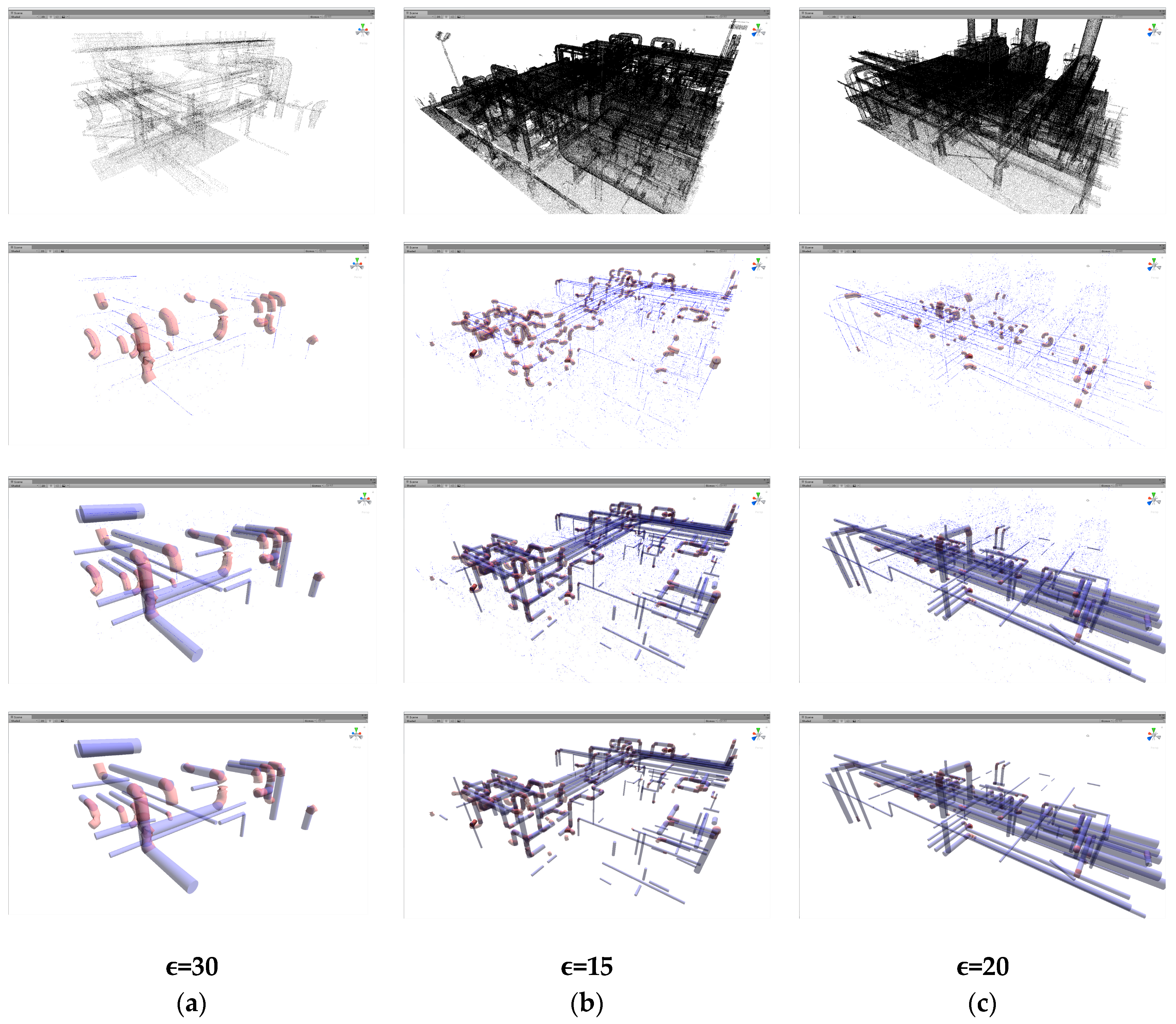
Figure 11 shows how the proposed method is applied in the segmented point cloud. Since the subject of this paper is to estimate the cylinder shape without normal estimation and segmentation, we verify the proposed method in point clouds where various types of nonsegmentation (railing, footing, valves, noise, etc.) exist.
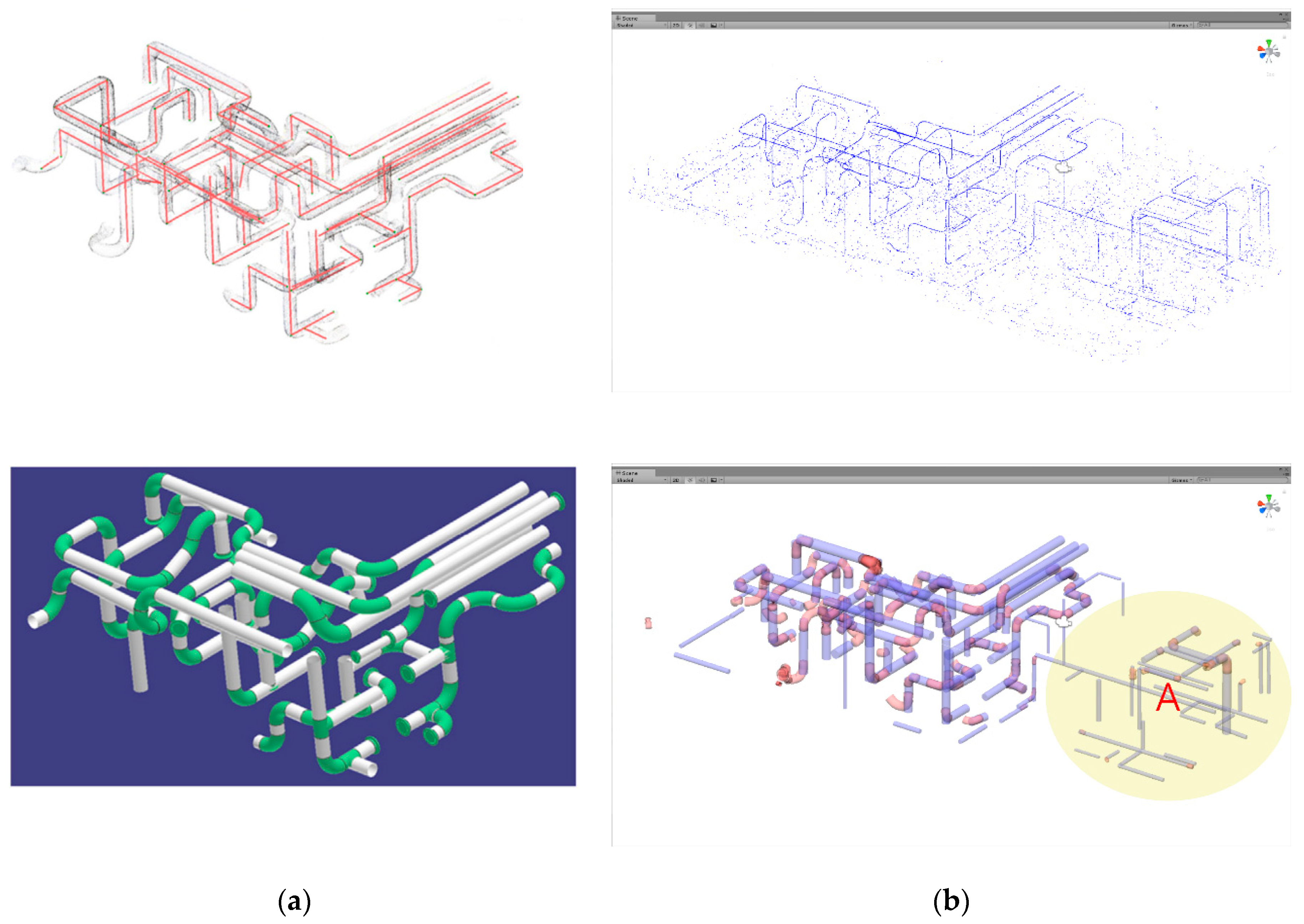
Figure 12a shows 103,498 points, Figure 12b shows 2,181,234 points, and Figure 11b shows the figure before segmentation. In Figure 12a, 6687 central axis estimation points and 1269 ms execution time were used for the central axis estimation, and 25 straight regions and 13 curved regions were estimated only for 1567 ms execution time. Both appear appropriate in terms of location. In strict criteria, there are 21 curved regions in Figure 12a.
Figure 12b constitutes the central axis points with execution times of 18,915 ms and 71,481, respectively, and an estimated 157/129 straight/curved regions. The execution time was 11,100 ms. In practice, there are about 200 pipes and about 200 bent areas. The estimated number of curved regions is relatively different because it is estimated that there is only one curved region (S-shape) leading from a 90° shape to a 90° shape again.
Figure 12c constitutes 52,385 central axis points with 1,984,708 data points, and it took 19,748 ms execution time. In total, 128 straight sections and 56 bent sections were found and the time required was 6075 ms. Compared to the other data, there was relatively more noise and many broken areas. Unfortunately, even though the chimney of the building was in the form of a cylinder, it could not be estimated. It is interpreted that the larger the diameter of the cylinder, the more the certain area is close to the plane, and a larger cylinder should search for more neighbors. The fitting ratios are shown in Table 1.
The reason why the linear ratio of Figure 12b in Table 1 is high is because one pipe is estimated to be a plurality of truncated pipes. Table 1 shows similar results even though there are differences in the size and density of data between Figure 12a and b. There are many cases where the pipe of the plant is constructed vertically/horizontally on the ground, but there are also cases where it is installed in a diagonal line, which means that additional calculation is necessary when constraints exist [9]. In addition, the bend area is calculated by finding the intersection point by extending the length from the result of finding the straight pipe and the 90° or T-shaped area. On the other hand, the proposed method can find not only vertical and horizontal regions, but also oblique regions, and S-shaped region estimation is also possible. The execution time is equal to O(n(P) n(L) n(E) c), where n(P) is the total number of data points, is the sphere fitting search increment, n(L) is the number of linear candidates/estimators, n(E) is the number of curved region candidates/estimators, and c is the evaluation cost. Eventually the appropriate value needs to be set in order to reduce execution time. In other words, the number of central axis data points determined by affects the amount of computation of n(L), n(E), and c. Therefore, the proper setting of has a great influence on overall performance.
In order to verify its efficiency, the proposed method using the data in Figure 12b compares/verifies the Hough transform method [10]. Figure 13 shows the left side of Figure 12b. Figure 13a shows the pipe estimation through the Hough transform [10], and Figure 13b shows no significant difference in the pipe estimation results by the proposed method.
Figure 13a shows an execution time of 591 s. Figure 13b shows that step 1 took 16 s and step 2 took 10 s. Therefore, it was 591/(16 + 10) = 22.73 times faster to estimate the pipe. A total of 89 left (CE) pipes exist in the left data, and the proposed method estimated 130 straight lines (CD) and 90 curves (CC). This seems to be better than the comparison of 60 CD. However, since the comparison object is estimated to have detected only the area of the top image of Figure 13a, the result of linear/curve estimation of the right area added in the top image of Figure 13b should be removed. The added right-hand region has about 50 straight lines and 15 curved lines. As a result, a straight line/curve of 80 (CD) and 75 (CC) was estimated. Here, the error is 10 (CF). This is a result of estimating a strict standard (constant length/position/angle). CD/CE is 0.9 and CT/CD is 0.88, which is somewhat greater than the 0.67 and 0.87 of the comparison subjects.
Figure 14 shows the right side of Figure 12b. Figure 14a shows that the execution time was 637 s. On the other hand, the proposed method took 19.5 s in step 1 and 17.5 s in step 2. The time required to estimate the pipe was 637/(17.5 + 19.5) = 17.21 times faster. The estimated straight line is 155, and the curve is 86. The number of pipes in the comparative thesis is 107 (CE), but the proposed method seems to have found too many. However, since the radius is estimated to be at least 8 inches, the number is reduced from 155 to 97 (CD). On the contrary, there are 72 (CD) in comparison. The CF of the proposed method is 14. Finally, CD/CE is 0.90 and CT/CD is 0.85. Compared with 0.67 and 0.88, CD/CE is higher and CT/CD is lower. The final results of Figure 13 and Figure 14 are shown in Table 2.
In Table 2, Rr (recall rate) is CT/CE, Er (error rate) is CF/CE, and Pr (precision rate) is CT/CD. The proposed method has a relatively high Rr because it limits the minimum radius of the pipe to 8 inches. There are more pipes in the actual data.
Er shows that the comparison method has better results. However, if the error is assumed to be the number not found in the whole of CE, Er = (CE-CT) / CE, the proposed method will be 0.21 and 0.22, and the comparison method will be 0.42 and 0.41. This is because the CT in the proposed method is larger than the comparison method. Also, if 8 inches of cylinders are not excluded, CE will be greater than 89, which will affect Rr and Er. The more pipes it is searched, the better way, so the new Er may be meaningful.
A cylinder of 8 inches or less is shown in Figure 13b (yellow circle A). These areas are cylinders with a radius of about 2 to 6 inches. Cylinders with small radii are difficult to estimate because their accuracy is low in sensor error and normal estimation. While the comparison method does not estimate the cylinder of this region, the proposed method shows some degree of cylinder estimation even though there are broken and missing parts. If CE contains less than 8 inches of cylinders, the proposed method will give better results in new Er. CE in Table 2 is in accordance with [10].
In the experiment of the proposed method, data is sampled by setting = 25 as the first line of pseudo code a. The central axis candidates can be obtained by repeatedly sphere fitting (error 1 cm) on the sampled 25% data (pseudo code a 2-4 lines). When the DCL is completed, average filtering is performed (Pseudo code a 5 lines). Once the filtered center axis candidates DFLT is computed, it is sampled 40% and the PCA is used to calculate the directionality of the local point cloud (pseudo code a 6-8 lines). The pseudo code b estimates the complete cylinders in the directional set . First, algorithm searches for a straight line candidate DEST that matches the angle (<15 degrees) and the distance (<15 cm) between the two vectors as shown in the third row. Since the retrieved DEST means one cylinder, the cylinder is completed using PCA as shown in the line 7. This process is repeated (pseudo code b 1-8 lines) to estimate all the cylinders. The pseudo code c is a code fitting the curve region. The DCYL is the estimated set of cylinders, and curves are retrieved from the based on the end points of each cylinder in the DCYL. The line 2 checks whether the discriminant is within a certain range through the surrounding points in the . When the discriminant value in the experiment is 0.02 ~ 0.06, it is determined as a curve. The straight line is 0.02 or less. Depending on how much noise the data contains, the line and curve discriminant values may have a certain overlapping range (ex: straight line 0.03, curve: 0.01 to 0.06). When the is in the curve range, lines 3-6 are the process of finding the intersection point by estimating the directionality at each neighboring point. If the intersection set DCP is a discriminant value 0.02 ~ 0.06, the DCP finally determines that it is a curve, sets the order of the control points, and finalizes it with the Catmull-Rom spline. Finally, the set of estimated curves is DSPL.
The compared method is an algorithm of structural characteristic that has the disadvantage of slower execution time as the number of data points increases. This is because the segmentation time increases. Also, pipes with small diameters require appropriate restrictions because the normal estimate is somewhat difficult. On the other hand, the proposed method is relatively fast and can maintain accuracy because there is no segmentation and a normal estimation procedure. The results of estimating the cylinder with proposed method by integrating Figure 13 and Figure 14 are in the Appendix.
The compared study uses the intersection point in the curved region estimation. Therefore, it is impossible to estimate an unfixed curved region. However, applying skeletonization may be able to estimate the bend area, but the opportunity cost will be increased accordingly. Skeletonization is mainly used with Laplacian smoothing [22] or L1-medial [23]/medial axis [24], and the opportunity cost of its application is likely to increase due to cylinder bending area loss and noise after object segmentation.
6. Conclusions
The method proposed in this paper shows that it is possible to estimate cylinder shape quickly in a point cloud. Sphere fitting was shown to be suitable for estimating the center axis of the cylinder, and the data were sampled for quick processing. The orientation of the constructed center axis data could be confirmed by PCA.
PCA can be assumed to be the tangent of the estimation curve, since the main directionality can be set from the dispersion of the point data. The intersection of these estimated tangent lines can be a control point of the Catmull–Rom spline, and the curve can be obtained through it. The more accurate the center line estimate through the sphere fitting is, the better the curve can be. However, PCA can be more robust against noise and is relatively fast and accurate compared to spline fitting. The distinction between a straight line and a curve can be easily distinguished by using Equation (6).
The proposed method has the advantage of estimating the linear/curved shape of the cylinder 10 times faster (22 times in Figure 13 and 17 times in Figure 14) than the comparison method while maintaining relative accuracy. In addition, more cylinders (less than 8 inches) were estimated. For center axis estimation, sphere fitting was performed with 1 cm error and using 25% data.
Of course, it can be quickly matched to the constraints through vertical/horizontal conditions, but there is a disadvantage in that the oblique pipe cannot be estimated. In addition, the estimation of the curve in the comparison method matches the intersection of two straight lines only in a defined form with a number of cases. On the other hand, since the proposed method estimates along the actual bent path, it can be processed according to angles of all bent shape. Of course, there is a clue that point data should be smoother.
The proposed method has its own merits, but there are disadvantages as well. When the density of point data is too high, it is necessary to search for more neighbors in order to process the curvature as a fit, which means the execution time is longer. Therefore, downsampling is required prior to cylinder fitting. Downsampling does not appear to be a major drawback, because it has a much lower opportunity cost than normal estimation or segmentation.
Reverse engineering of construction modeling requires a lot of manual work. The more data there is, the harder it is for the operator to recognize the shape of the object. In other words, the more objects to recognize, the narrower the distance between objects, and the more difficult it is to distinguish objects on 2D screens. Therefore, fast recognition of primitive shapes is a good way to increase work efficiency. If it is forced to be accompanied by manual labor, it may be an effective alternative to obtain relatively quick estimation results rather than perfect automation. This paper is expected to improve the working efficiency of linear and curved cylinder estimation after center axis estimation without constraints and segmentation. Further study will be conducted in a way that smoothly integrates the estimated straight lines and curved parts into one and can produce consistent results.
Author Contributions
Conceptualization, Y.-H.J.; Methodology, Y.-H.J.; Software, Y.-H.J.; Supervision, W.-H.L.; Visualization, Y.-H.J.; Writing—original draft, Y.-H.J.; Writing—review & editing, Y.-H.J.
Conflicts of Interest
The authors declare no conflict of interest.
Appendix A
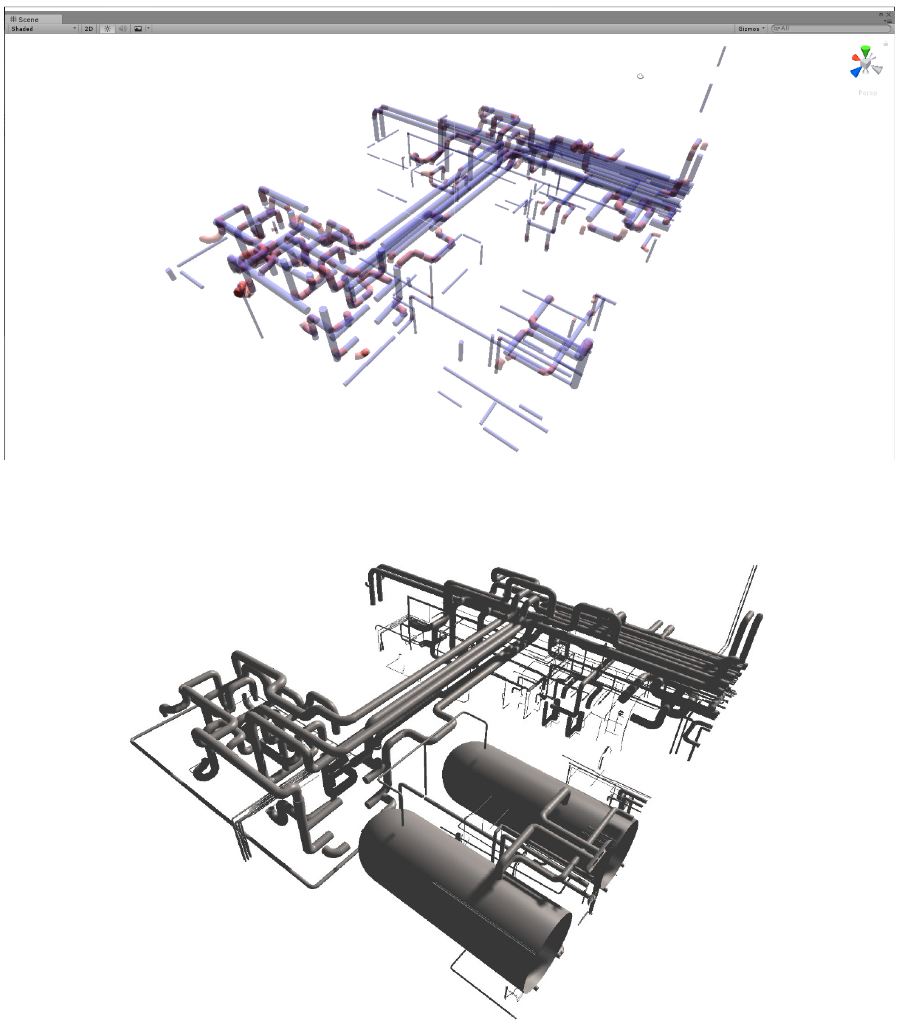
Figure A1.
This figure is the result of modeling the point cloud data of Figure 12b by a human. The proposed method resulted in about 1 minute of execution time.
Figure A1.
This figure is the result of modeling the point cloud data of Figure 12b by a human. The proposed method resulted in about 1 minute of execution time.


References
- Rabbani, T.; van den Heuvel, F.; Vosselmann, G. Segmentation of point clouds using smoothness constraint. ISPRS 2006, 36, 248–253. [Google Scholar]
- Rabbani, T.; Van Den Heuvel, F. Efficient though transform for automatic detection of cylinders in point clouds. ISPRS 2005, 3, 60–65. [Google Scholar]
- Schnabel, R.; Wahl, R.; Klein, R. Efficient RANSAC for Point-Cloud Shape Detection. Comput. Graph. Forum 2007, 26, 214–226. [Google Scholar] [CrossRef] [Green Version]
- Abuzaina, A.; Nixon, M.S.; Carter, J.N. Sphere detection in kinect point clouds via the 3d hough transform. In Proceedings of the International Conference on Computer Analysis of Images and Patterns (CAIP); Springer: Berlin/Heidelberg, Germany, 2013; pp. 290–297. [Google Scholar]
- Zhang, N. Plane Fitting on Airborne Laser Scanning Data Using RANSAC; Lunds Tekniska Högskola Universitet: Lund, Sweden, 2011; Available online: http://www.maths.lth.se/matematiklth/personal/petter/rapporter/plane fitting.pdf (accessed on 6 March 2019).
- Garcia, S. Fitting Primitive Shapes to Point Clouds for Robotic Grasping. Master’s Thesis, School of Computer Science and Communication, Royal Institute of Technology, Stockholm, Sweden, 2009. [Google Scholar]
- Su, Y.-T.; Bethel, J. Detection and robust estimation of cylinder features in point clouds. In Proceedings of the ASPRS Annual Conference on Opportunities for Emerging Geospatial Technologies, San Diego, CA, USA, 26–30 April 2010. [Google Scholar]
- Jones, B.; Aoun, M. Learning 3D Point Cloud Histograms; CS 229 Machine Learning Final Projects; Stanford University: Stanford, CA, USA, 2009; Available online: http://cs229.stanford.edu/proj2009/JonesAoun.pdf (accessed on 6 March 2019).
- Liu, Y.J.; Zhang, J.B.; Hou, J.C.; Ren, J.C.; Tang, W.Q. Cylinder detection in large-scale point cloud of pipeline plant. IEEE Trans. Vis. Comput. Graph. 2013, 19, 1700–1707. [Google Scholar] [CrossRef] [PubMed]
- Patil, A.K.; Holi, P.; Lee, S.K.; Chai, Y.H. An adaptive approach for the reconstruction and modeling of as-built 3D pipelines from point clouds. Autom. Constr. 2017, 75, 65–78. [Google Scholar] [CrossRef]
- Ahmed, M.F.; Haas, C.T.; Haas, R. Automatic detection of cylindrical objects in built facilities. J. Comput. Civ. Eng. 2014, 28, 04014009. [Google Scholar] [CrossRef]
- Son, H.; Kim, C.; Kim, C. Automatic 3D reconstruction of as-built pipeline based on curvature computations from laserscanned data. In Proceedings of the Construction Research Congress, Atlanta, GA, USA, 19–21 May 2014; pp. 925–934. [Google Scholar]
- Huang, J.; You, S. Detecting objects in scene point cloud: A combinational approach. In Proceedings of the 2013 International Conference on 3D Vision—3DV 2013, Seattle, WA, USA, 29 June–1 July 2013. [Google Scholar]
- Pang, G.; Qiu, R.; Huang, J.; You, S.; Neumann, U. Automatic 3D industrial point cloud modeling and recognition. In Proceedings of the 2015 14th IAPR International Conference on MVA, Tokyo, Japan, 18–22 May 2015; pp. 22–25. [Google Scholar]
- Qiu, R.; Zhou, Q.-Y.; Neumann, U. Pipe-run extraction and reconstruction from point clouds. In Proceedings of the ECCV, Zurich, Switzerland, 6–12 September 2014; pp. 17–30. [Google Scholar]
- Fischler, M.A.; Bolles, R.C. Random sample consensus: A paradigm for model fitting with applications to image analysis and automated cartography. Commun. ACM 1981, 24, 381–395. [Google Scholar] [CrossRef]
- Wikipedia. Available online: https://en.wikipedia.org/wiki/RANSAC (accessed on 24 February 2019).
- Smith, L.I. A Tutorial on Principal Components Analysis; Otago University: Dunedin, New Zealand, 2002. [Google Scholar]
- Wikipedia. Available online: https://en.wikipedia.org/wiki/Principal_component_analysis (accessed on 24 February 2019).
- Wikipedia. Available online: https://en.wikipedia.org/wiki/Spline_(mathematics) (accessed on 24 February 2019).
- Twigg, C. Catmull-rom splines. Computer 2003, 41, 4–6. [Google Scholar]
- Au, O.K.C.; Tai, C.L.; Chu, H.K.; Cohen-Or, D.; Lee, T.Y. Skeleton extraction by mesh contraction. ACM Trans. Graph. 2008, 27, 44. [Google Scholar] [CrossRef]
- Huang, H.; Wu, S.; Cohen-Or, D.; Gong, M.; Zhang, H.; Li, G.; Chen, B. L1-medial skeleton of point cloud. ACM Trans. Graph. 2013, 32, 65. [Google Scholar] [CrossRef]
- Tagliasacchi, A.; Zhang, H.; Cohen-Or, D. Curve skeleton extraction from incomplete point cloud. ACM Trans. Graph. 2009, 28, 71. [Google Scholar] [CrossRef]
Figure 1.
(a) Model recognition preprocessing process; (b) region growing segmentation [1].
Figure 1.
(a) Model recognition preprocessing process; (b) region growing segmentation [1].

Figure 2.
Center estimation using the trace of a sphere.

Figure 3.
PCA eigenvector estimation.

Figure 4.
(a) Neighboring points and fitting results for spherical fitting. (b) Outlier removal through local averaging. (c) Sphere fitting using six points in cross-section. (d) Neighboring point search. (e) Average filter processing result.
Figure 4.
(a) Neighboring points and fitting results for spherical fitting. (b) Outlier removal through local averaging. (c) Sphere fitting using six points in cross-section. (d) Neighboring point search. (e) Average filter processing result.

Figure 5.
Matching execution time and results according to matching increase value: (a) segmented data, (b) full data.
Figure 5.
Matching execution time and results according to matching increase value: (a) segmented data, (b) full data.


Figure 6.
Estimating the accuracy of matching results: (a) CloudCompare point distance; (b) proposed method diameter.
Figure 6.
Estimating the accuracy of matching results: (a) CloudCompare point distance; (b) proposed method diameter.

Figure 7.
Search method for center axis estimation: (a) eigenvector at a point; (b) sum of eigenvectors; (c) matching cylinder result through vector summation.
Figure 7.
Search method for center axis estimation: (a) eigenvector at a point; (b) sum of eigenvectors; (c) matching cylinder result through vector summation.

Figure 8.
Control point estimation using PCA: (a) estimation of tangent line at one point; (b) estimation of spline control point using intersection of tangent line; (c) curve matching result.
Figure 8.
Control point estimation using PCA: (a) estimation of tangent line at one point; (b) estimation of spline control point using intersection of tangent line; (c) curve matching result.

Figure 9.
Change of curve according to : red 0.2, black 0.5, green 0.75 [21].
Figure 9.
Change of curve according to : red 0.2, black 0.5, green 0.75 [21].

Figure 10.
Control point alignment for Catmull–Rom spline: (a) aligned control points; (b) unaligned control points; (c) control point alignment through PCA.
Figure 10.
Control point alignment for Catmull–Rom spline: (a) aligned control points; (b) unaligned control points; (c) control point alignment through PCA.

Scheme 1.
Pseudo Code for proposed method: (a) sphere fitting; (b) straight lines estimation; (c) curves estimation.
Scheme 1.
Pseudo Code for proposed method: (a) sphere fitting; (b) straight lines estimation; (c) curves estimation.

Figure 11.
Estimation from segmented data with ϵ. From the left: point cloud/curved, center axis/straight, and curved areas: (a) simple data; (b) complicated data.
Figure 11.
Estimation from segmented data with ϵ. From the left: point cloud/curved, center axis/straight, and curved areas: (a) simple data; (b) complicated data.

Figure 12.
Estimation from nonsegmented data with . From top: point cloud/bent area, center axis/bent area, center axis, straight/final result mapping: (a) simple data; (b) complicated data 1; (c) complicated data 2.
Figure 12.
Estimation from nonsegmented data with . From top: point cloud/bent area, center axis/bent area, center axis, straight/final result mapping: (a) simple data; (b) complicated data 1; (c) complicated data 2.

Figure 13.
Comparison of proposed method with actual data (left side of Figure 12b). From top to bottom: point cloud/cylinder matching/center axis/final result. (a) Estimation by Hough transform [10]; (b) estimation by proposed method.


Figure 14.
Comparison of proposed method with actual data (right side of Figure 12b). From top to bottom: point cloud/cylinder matching/center axis/final result. (a) Estimation by Hough transform [10]; (b) estimation by proposed method.


Table 1.
Results in Figure 12 (unit: number).
Table 1.
Results in Figure 12 (unit: number).
| Figure 12a | Figure 12b | Figure 12c | ||||
|---|---|---|---|---|---|---|
| Line | Curve | Line | Curve | Line | Curve | |
| Real No. | 30 | 21 | 200 | 200 | 170 | 88 |
| Correct No. | 25 | 13 | 157 | 129 | 128 | 56 |
| Ratio | 0.833 | 0.619 | 0.785 | 0.645 | 0.752 | 0.636 |
Table 2.
Comparison verification. CE, actual pipe number; CD, estimated pipe number; CT, estimated success number; CF, estimated failure number; t, run time; Rr, recall rate; Er, error rate; Pr, precision rate.
Table 2.
Comparison verification. CE, actual pipe number; CD, estimated pipe number; CT, estimated success number; CF, estimated failure number; t, run time; Rr, recall rate; Er, error rate; Pr, precision rate.
| Model | CE | Proposed | Compared [10] | ||||||||||||
|---|---|---|---|---|---|---|---|---|---|---|---|---|---|---|---|
| CD | CT | CF | Rr | Er | Pr | t | CD | CT | CF | Rr | Er | Pr | t | ||
| Figure 13 (Left) | 89 | 80 | 70 | 10 | 0.79 | 0.11 | 0.88 | 25 s | 60 | 52 | 8 | 0.58 | 0.09 | 0.86 | 591 s |
| Figure 14 (Right) | 107 | 97 | 83 | 14 | 0.78 | 0.13 | 0.85 | 37 s | 72 | 63 | 9 | 0.59 | 0.08 | 0.88 | 637 s |
© 2019 by the authors. Licensee MDPI, Basel, Switzerland. This article is an open access article distributed under the terms and conditions of the Creative Commons Attribution (CC BY) license (http://creativecommons.org/licenses/by/4.0/).
Share and Cite
MDPI and ACS Style
Jin, Y.-H.; Lee, W.-H. Fast Cylinder Shape Matching Using Random Sample Consensus in Large Scale Point Cloud. Appl. Sci. 2019, 9, 974. https://doi.org/10.3390/app9050974
AMA Style
Jin Y-H, Lee W-H. Fast Cylinder Shape Matching Using Random Sample Consensus in Large Scale Point Cloud. Applied Sciences. 2019; 9(5):974. https://doi.org/10.3390/app9050974
Chicago/Turabian StyleJin, Young-Hoon, and Won-Hyung Lee. 2019. "Fast Cylinder Shape Matching Using Random Sample Consensus in Large Scale Point Cloud" Applied Sciences 9, no. 5: 974. https://doi.org/10.3390/app9050974
Note that from the first issue of 2016, this journal uses article numbers instead of page numbers. See further details here.