Tensor Robust Principal Component Analysis via Non-Convex Low Rank Approximation

Abstract

Tensor Robust Principal Component Analysis (TRPCA) plays a critical role in handling high multi-dimensional data sets, aiming to recover the low-rank and sparse components both accurately and efficiently. In this paper, different from current approach, we developed a new t-Gamma tensor quasi-norm as a non-convex regularization to approximate the low-rank component. Compared to various convex regularization, this new configuration not only can better capture the tensor rank but also provides a simplified approach. An optimization process is conducted via tensor singular decomposition and an efficient augmented Lagrange multiplier algorithm is established. Extensive experimental results demonstrate that our new approach outperforms current state-of-the-art algorithms in terms of accuracy and efficiency.

1. Introduction

An array of numbers arranged on a regular grid with a variable number of axes is described as a tensor. As the dimensionality reaches beyond 3D, conventional data representations such as vector-based and matrix-based become insufficient, and highly dimensional data sets are usually formulated as tensors [1,2,3].

Robust Principal Component Analysis (RPCA) [4,5,6,7,8], aiming to recover the low-rank and sparse matrices both accurately and efficiently, has been widely studied in data compressed sensing and computer vision. It is of great use when we try to solve the problem of subspace learning or Principal Component Analysis (PCA) in the presence of outliers [9]. Especially RPCA is a very useful tool in foreground detection, which is the first step in video surveillance system to detect moving objects [10,11]. Tensor Robust Principal Component Analysis (TRPCA) extends the RPCA from matrix to the tensor case, that is, to recover a low-rank tensor and a sparse (noise entries) tensor.

Tensor rank [12] essentially characterizes the intrinsic "dimension” or “degree of freedom” for highly dimensional data sets. In order to make the rank characteristic be more transparent, one can make use of tensor Singular Value Decomposition (t-SVD) developed recently by Kilmer and Martin [13], rendering the tensor rank approximation approachable. The key for their framework is the well-defined t-product that leads to the 3rd-order tensor space to be an inner product space so that approximation becomes more effective such as in image processing [14,15]. t-SVD allows to define tensor tubal-rank, which appears to be much more approachable such as in the study of image analysis than previous rank definitions [16,17,18]. The characteristic of a low tensor tubal-rank implies that a 3rd-order tensor can be significantly compressed (Theorem 4.3 of [13]), which is particularly important in applications.

Mathematically, TRPCA based on t-SVD [19,20] aims to recover the low tubal rank component ${\mathcal{L}}_0$ and sparse component ${\mathcal{E}}_0$ from noisy observations $\mathcal{X}={\mathcal{L}}_0+{\mathcal{E}}_0$ of size $N_1\times N_2\times N_3$ by convex optimization

$$\begin{array}{cc}\hfill \underset{\mathcal{L},\mathcal{E}}{min}& {\parallel \mathcal{L}\parallel }_{TNN}+\lambda {\parallel \mathcal{E}\parallel }_{{\ell }_1}\hfill \end{array}$$

(1)

$$\begin{array}{cc}\hfill \mathrm{s}.\mathrm{t}.& \mathcal{X}=\mathcal{L}+\mathcal{E}.\hfill \end{array}$$

(2)

$\lambda$ is a Lagrange multiplier, $\mathcal{E}$ is sparse if the tensor ${\ell }_1$ norm ${\parallel \mathcal{E}\parallel }_{{\ell }_1}$ is small. It is well-known that the t-SVD-based tensor nuclear norm (TNN, III.B of [21]) has been proven to be the tightest convex relaxation to ${\ell }_1$-norm of the tensor multi-rank (Theorem 2.4.1 in [15] or Theorem 3.1 in [19]). However, TNN treats the singular values in t-SVD equally to pursue the convexity of the objective function, while the singular values associated with a practical image may emphasize its different properties and should be handled differently, in particular, when some singular values are very large. Due to the gap between the tensor rank function and its lower convex envelop, the adoption of tensor nuclear norm may lead to the approximation of the corresponding tensor tubal-rank being inaccurate. Therefore, a new development of tensor tubal-rank approximation becomes necessary to reflect these fundamental characteristics.

To make the the necessity of a new tensor tubal-rank approximation instead of TNN more transparent, we consider the the matrix RPCA [4] first. Now the goal becomes to recover a low-rank matrix L from highly corrupted observations $X=L+S,$ by minimizing ${\parallel L\parallel }_{*}+\lambda {\parallel S\parallel }_{{\ell }_1}$. Here ${\parallel L\parallel }_{*}$ is the summation of the singular values of L. It is easy to see that

$$1+\frac{{\sigma }_2}{{\sigma }_1}+\cdots +\frac{{\sigma }_N}{{\sigma }_1}=\frac{1}{{\sigma }_1}{\parallel L\parallel }_{*}\le \mathrm{rank}(L).$$

Hence, when ${\sigma }_1$ is very large, for example, and the rest are relatively small, we may have $\frac{1}{{\sigma }_1}{\parallel L\parallel }_{*}<<$ rank$(L)$. Then the minimization of ${\parallel L\parallel }_{*}$ will attempt to minimize ${\sigma }_1$ that leads to over-penalizes ${\sigma }_1$, and consequently it generates undesirable solution L with small ${\sigma }_1$. Recall that our goal is to find a low-rank L, whose largest singular value is not necessarily to be small. In addition, it is worth mentioning that in practice the matrix RPCA problem is very sensitive to small perturbations and this problem can be addressed by relaxing the equality constraints. The authors in [22,23] propose an alternative optimization approach that appears to be suitable to deal with robustness issues in the “Sparse Plus Low-rank” decomposition problem. It has long been noticed that the nuclear norm is not always satisfactory [24], since it over-penalizes large singular values, and consequently may only find a much biased solution. Since the the nuclear norm is the tightest convex relaxation of the rank function [25], a further improvement under the convex setting in general is limited, if it is still possible, in particular when their gap is not very small. In order to alleviate the above problem, the Gamma quasi-norm for matrices is introduced in [26] in RPCA, which results in a tighter approximation of the rank function. For $L\in {\mathbb{R}}^{m\times n}$ and the singular values of L, denoted by ${\sigma }_1(L),\dots ,{\sigma }_{min\{m,n\}}(L)$, the Gamma quasi-norm of L is defined as

$${||L||}_{\gamma }=\sum _{i=1}^{min\{m,n\}}\frac{(1+\gamma ){\sigma }_i(L)}{\gamma +{\sigma }_i(L)},\gamma >0.$$

It is not difficult to see

$$\frac{(1+\gamma ){\sigma }_i(L)}{\gamma +{\sigma }_i(L)}<\frac{1+\gamma }{\gamma +M}{\sigma }_i(L),$$

when ${\sigma }_i(L)>M>0$ and ${||L||}_{\gamma }\le (1+\gamma )\mathrm{rank}(L).$ So it overcomes the imbalanced penalization by different singular values in convex nuclear norm. In addition, when $\gamma$ goes to 0, the limit of the Gamma quasi-norm is exactly the matrix rank. The Gamma quasi-norm has nice algebraic properties, i.e., unitarily invariant and positive definiteness. Thanks to the unitarily invariance [27], the Gamma quasi-norm minimization problem for $A\in {\mathbb{R}}^{m\times n}$:

$$\underset{Z\in {\mathbb{R}}^{m\times n}}{min}{||Z||}_{\gamma }+\frac{\mu }{2}{∥Z-A∥}_F^2$$

can be solved very effectively (Theorem 1 of [26]). Moreover, experimental results in [26] show that Gamma quasi-norma-based RPCA outperforms several other convex/non-convex norma-based RPCA in both accuracy and efficiency.

In this paper, inspired by the success of the non-convex rank approximation [26], we proposed tensor Gamma quasi-norm via t-SVD to seek a closer approximation and to alleviate the above-mentioned limitations resulted from the tensor nuclear norm, which has not been used for TRPCA yet in literature.

The main contributions of this paper are illustrated as follows:

• We develop new non-convex tensor rank approximation functions that can be used as desirable regularization for the optimization process, which appears to be more effective than current existing approaches in literature.  
• An efficient algorithm based on the alternating direction method of multipliers (ADMM) is developed to solve the equivalent optimization problem in the Fourier domain, which is also suitable for general TRPCA problem. In addition, we provided the convergent analysis of the augmented Lagrange multiplier based optimization algorithm.  
• Extensive evaluation of the proposed approach on several benchmark data sets has been conducted, and detailed comparison with most recent approaches are provided. Experimental results demonstrate that our proposed approach yields superior performance for image recovery and video background modeling.

The rest of the paper is organized as follows. In Section 2, we roughly describe some related works. Then Section 3 provides factorization strategies for 3rd-order tensors and its relationship to the corresponding tensor approximation problem. And then we present the main results on t-Gamma quasi-norm of 3rd-order tensors. Section 4 introduces our non-convex TRPCA framework and the convergent analysis of the augmented Lagrange multiplier based optimization algorithm. Experimental analysis and results are shown in Section 5 to verify the proposed algorithm. Finally, the paper ends with concluding remarks in Section 6.

2. Related Works

Recently, many authors observed the limitations of t-SVD-based TRPCA [15,19]. It was pointed out in [28] that the classical TRPCA methods based on t-SVD fails to utilize the low rank structure in the third mode. To further exploit the low-rank structures in multiway data, they defined a new TNN that extends TNN with core matrix and proposed a creative algorithm to deal with TRPCA problems. In addition, the authors of [29] presented that there are some weak points in the existing low-rank approximation approaches, for example, people need to predefine the rank values or fail to consider local information of data (e.g., spatial or spectral smooth structure). So they proposed a novel TNN-based low-rank approximation with total variation regularization, which uses the TNN to encode the global low-rank prior of tensor data and the total variation regularization to preserve the spatial-spectral continuity in a unified framework.

It has been noticed by others that TNN is not always satisfactory. For instance, to seek a closer approximation of tensor rank, Kong et al. in [30] introduced t-Schatten-p tensor quasi-norm to replace the TNN. The t-Schatten-p norm is convex when $p\ge 1$, but non-convex when $0<p<1$. In addition, they proved multi-Schatten-p norm surrogate theorem to convert the non-convex t-Schatten-p tensor quasi-norm for $0<p<1$ into a weighted sum of convex functions. Then based on the multi-Schatten-p norm surrogate, they proposed a novel convex tensor RPCA model.

Besides above, a recent paper [31] developed randomized algorithms for tensor low-rank approximation and decomposition, together with tensor multiplication. Their proposed tubal focused algorithms employ a small number of lateral and/or horizontal slices of the underlying 3rd order tensor, that come with relative error guarantees for the quality of the obtained solutions.

Besides the above-mentioned methods based on t-SVD, there are many other TRPCA methods mainly applied CP (CANDECOMP/PARAFAC) or Tucker decompositions methods in their optimization models. We need to mention that recently Driggs et al. [32] studied TRPCA using a non-convex formulation of the CP based tensor atomic-norm and identified a class of local minima of this non-convex program that are globally optimal.

Presently, background subtraction become more and more important for visual surveillance systems and several subspace learning algorithms based on matrix and tensor tools have been used to perform the background modeling of the scenes. Recently, Sobral et al. [33] developed an incremental tensor subspace learning that uses only a small part of the entire data and updates the low-rank model incrementally when new data arrives and in [34] the authors proposed an online stochastic framework for tensor decomposition of multispectral video sequences. In particular, it is worth mentioning that Bouwmans et al. [35] gave a systematic and complete review of the "low-rank plus sparse matrix decomposition" framework of separating moving objects from the background.

However, all those above mentioned t-SVD-based TRPCA algorithms solve the TRPCA optimization problem under convex regularization. In addition, most analyses of ADMM algorithms are in the convex setting [36]. In our work, we explore the TRPCA method based on the non-convex t-Gamma quasi-norm of 3rd-order tensors. Due to the non-convex nature of our TRPCA model, the convergent analysis of algorithm is difficult to justify. In addition, the analysis of non-convex augmented Lagrangians is not easy, but this compels us to make efforts of clarity and pedagogy. Also it should be noted that there are few works on t-SVD-based TRPCA achieve background modeling. Thus experiments are provided in our paper on two computer vision applications, which are image recovery and video background modeling.

3. Notations and Definitions

Throughout this paper, all boldface Euler script letters ($\mathcal{X}$) denote tensors, uppercase characters (X) denote matrices, and lowercase letters (a) denote scalars. The field of real numbers is denoted as $\mathbb{R}$. We denote $N_i,i=1,2,3$ as the index set associated with a given tensor. For 3rd-order tensors $\mathcal{X}=\left[a_{ijk}\right]\in {\mathbb{R}}^{N_1\times N_2\times N_3}$, we use $\mathcal{X}(i,:,:)$, $\mathcal{X}(:,i,:)$, $\mathcal{X}(:,:,i)$ to denote the i-th horizontal, lateral, and frontal slice, respectively. For simplicity, we denote the frontal slice $\mathcal{X}(:,:,i)$ as $X_i$. The inner product between $\mathcal{X}$ and $\mathcal{Y}$ of size $N_1\times N_2\times N_3$ is defined as $\langle \mathcal{X},\mathcal{Y}\rangle ={\sum }_{i=1}^{N_3}\mathrm{tr}(X_i^T{Y}_i)$. The Frobenius norm of a tensor is defined as ${∥\mathcal{X}∥}_F=\sqrt{{\sum }_{i,j,k}{\left|a_{ijk}\right|}^2}$. The ${\ell }_1$ norm of a tensor is defined as ${∥\mathcal{X}∥}_{{\ell }_1}={\sum }_{i,j,k}\left|a_{ijk}\right|$. In this paper, the adopted basic definitions and notations follow the references [13,21,37] for the purpose of an easier comparison.

Definition 1

(Transpose p. 10 of [13]). For $\mathcal{X}\in {\mathbb{R}}^{N_1\times N_2\times N_3}$, the transpose tensor ${\mathcal{X}}^{\mathrm{T}}$ is an $N_2\times N_1\times N_3$ tensor obtained by transposing each frontal slice of $\mathcal{X}$ and then reversing the order of the transposed frontal slices 2 through $N_3$.

Similar to matrices whose elements can be grouped by rows or by columns, higher dimensional tensors can be viewed forming by slices along the third mode. For $\mathcal{X}=[X_1|\cdots |X_{N_3}]\in {\mathbb{R}}^{N_1\times N_2\times N_3}$ with $N_1\times N_2$ frontal slices $X_1,\dots ,X_{N_3}$. Then the block circulant is created from the frontal slices in a form of

$$\begin{array}{c}\hfill \mathrm{bcirc}(\mathcal{X})=\left[\begin{array}{ccccc}{X}_1& X_{N_3}& X_{N_3-1}& \cdots & X_2\\ X_2& X_1& X_{N_3}& \cdots & X_3\\ ⋮& ⋮& ⋮& ⋮& ⋮\\ X_{N_3}& X_{N_3-1}& \cdots & X_2& X_1\end{array}\right],\end{array}$$

where $X_i=\mathcal{X}(:,:,i)$ for $i=1,\dots ,N_3$. It is important to notice that the block circulant matrix bcirc$(\mathcal{X})$ keeps the order of frontal slices of $\mathcal{X}$ in an appropriate way, and thus it better maintains $\mathcal{X}$’s structure in terms of the frontal direction, compared with the direct tensor unfolding along the third mode.

Definition 2

(t-product p. 11 of [13]). Let $\mathcal{X}\in {\mathbb{R}}^{N_1\times N_2\times N_3}$, we define the matvec and fold operators as $matvec(\mathcal{X})=\left[X_1;X_2;\cdots ;X_{N_3}\right]$ is an $N_1{N}_3\times N_2$ matrix and $fold(matvec(\mathcal{X}))=\mathcal{X}$.

Let $\mathcal{A}\in {\mathbb{R}}^{N_1\times N_4\times N_3}$, and $\mathcal{B}\in {\mathbb{R}}^{N_4\times N_2\times N_3}$. Then the t-product of 3rd-order tensors is defined as

$$\mathcal{A}*\mathcal{B}=fold(bcirc(\mathcal{A})matvec(\mathcal{B}))$$

which is a tensor of size $N_1\times N_2\times N_3$.

Definition 3

(Identity, orthogonal and diagonal tensor p.10 of [13]). The identity tensor $\mathcal{I}\in {\mathbb{R}}^{N_1\times N_1\times N_3}$ is a tensor whose first frontal slice is the $N_1\times N_1$ identity matrix and all other frontal slices are zero. A tensor $\mathcal{Q}\in {\mathbb{R}}^{N_1\times N_1\times N_3}$ is orthogonal if ${\mathcal{Q}}^{\mathrm{T}}*\mathcal{Q}=\mathcal{Q}*{\mathcal{Q}}^{\mathrm{T}}=\mathcal{I},$ where * is the t-product. A tensor is called f-diagonal if each of its frontal slices is diagonal matrix.

It is well known that circulant matrices can be diagonalized by the FFT (21.11 of [38]), similarly, block-circulant matrices can also block-diagonalized as

$$\begin{array}{cc}& \left({\tilde{\mathbf{F}}}_{N_3}\otimes {\mathbf{I}}_{N_1}\right)·\mathrm{bcirc}(\mathcal{X})·\left({\tilde{\mathbf{F}}}_{N_3}^{*}\otimes {\mathbf{I}}_{N_2}\right)\hfill \\ \hfill =& \mathrm{bdiag}(\widehat{\mathcal{X}})=\left[\begin{array}{ccc}{\widehat{X}}_1& & \\ & \ddots & \\ & & {\widehat{X}}_{N_3}\end{array}\right],\hfill \end{array}$$

where ${\tilde{\mathbf{F}}}_{N_3}=\frac{1}{\sqrt{N_3}}{\mathbf{F}}_{N_3}$, ${\mathbf{F}}_{N_3}$ denotes the $N_3\times N_3$ fast Fourier transform matrix, ${\mathbf{F}}_{N_3}^{*}$ denotes its conjugate, and the notation ⊗ denotes the standard Kronecker product. In addition, $\mathcal{X}=\mathcal{A}*\mathcal{B}$ if and only if ${\widehat{X}}_{n_3}={\widehat{A}}_{n_3}{\widehat{B}}_{n_3}$ for $1\le n_3\le N_3$ (p.4 of [19]).

Since ${\tilde{\mathbf{F}}}_{N_3}\otimes {\mathbf{I}}_{N_1},{\tilde{\mathbf{F}}}_{N_3}\otimes {\mathbf{I}}_{N_2}$ are unitary matrices, we have

$$\parallel \mathrm{bdiag}(\widehat{\mathcal{X}}){\parallel }_F^2=\mathrm{tr}\mathrm{bcirc}{(\mathcal{X})}^T\mathrm{bcirc}(\mathcal{X})=N_3{||\mathcal{X}||}_F^2.$$

Then we have $\parallel \mathcal{X}{\parallel }_F=\frac{1}{\sqrt{N_3}}\parallel \mathrm{bdiag}(\widehat{\mathcal{X}}){\parallel }_F$.

Definition 4

(Tensor multi-rank p. 10 of [37]). For tensor $\mathcal{X}\in {\mathbb{R}}^{N_1\times N_2\times N_3}$ with $N_1\times N_2$ frontal slices $X_1,\dots ,X_{N_3}$, the multi-rank of $\mathcal{X}$ is a $N_3$-vector $[rank({\widehat{X}}_1),\dots ,rank({\widehat{X}}_{N_3})],$ consisting of the ranks of all the ${\widehat{X}}_1,\dots ,{\widehat{X}}_{N_3}$.

Please note that the matrix SVD [39] can be performed on each frontal slice of $\widehat{\mathcal{X}}$, The matrix ${\widehat{X}}_{n_3}$ has the following Singular Value Decomposition (SVD) ${\widehat{X}}_{n_3}={\widehat{U}}_{n_3}{\widehat{\mathsf{\Sigma }}}_{n_3}{\widehat{V}}_{n_3}^{\mathrm{T}},{\widehat{U}}_{n_3}\in \mathbb{O}(N_1),{\widehat{V}}_{n_3}\in \mathbb{O}(N_2)$ (here $\mathbb{O}(N_i)$ stands for the set of orthogonal $N_i$-by-$N_i$ matrices) and ${\widehat{\mathsf{\Sigma }}}_{n_3}$ is an $N_1\times N_2$ diagonal matrix with diagonal entries ${\sigma }_1({\widehat{X}}_{n_3}),\dots ,{\sigma }_{min\{N_1,N_2\}}({\widehat{X}}_{n_3})$ in descending order.

Definition 5

(t-SVD, Theorem 4.1 in [13]). The tensor Singular Value Decomposition (t-SVD) of $\mathcal{X}$ is given by $\mathcal{X}=\mathcal{U}*\mathsf{\Sigma }*{\mathcal{V}}^{\mathrm{T}},$ where $\mathcal{U}$ and $\mathcal{V}$ are orthogonal tensors of size $N_1\times N_1\times N_3$ and $N_2\times N_2\times N_3$ respectively. Σ is an f-diagonal tensor of size $N_1\times N_2\times N_3$, and * denotes the t-product.

Definition 6

(Tensor tubal rank III.B of [21]). The tensor tubal rank is defined as the number of nonzero singular tubes of f-diagonal tensor Σ, which is the maximum of the number of nonzero $\{{\widehat{\mathsf{\Sigma }}}_{n,n,n_3},1\le n\le min(N_1,N_2)\}$ for $1\le n_3\le N_3$.

Definition 7

(Tensor nuclear norm III.B of [21]). The nuclear norm for a given 3rd-order tensor $\mathcal{X}\in {\mathbb{R}}^{N_1\times N_2\times N_3}$ is defined to be

$$\parallel \mathcal{X}{\parallel }_{TNN}=\frac{1}{N_3}\sum _{n_3=1}^{N_3}||{\widehat{X}}_{n_3}{||}_{*},$$

which is equal to

$$\sum _{n=1}^{min(N_1,N_2)}\sum _{n_3=1}^{N_3}\frac{1}{N_3}{\widehat{\mathsf{\Sigma }}}_{n,n,n_3}.$$

Here ${\widehat{X}}_{n_3}$ is the $n_3$-th frontal slice of $\widehat{\mathcal{X}}=\mathrm{fft}(\mathcal{X},\left[\right],3)=[{\widehat{X}}_1|\cdots |{\widehat{X}}_{N_3}]\in {\mathbb{R}}^{N_1\times N_2\times N_3}$ obtained by applying FFT on $\widehat{\mathcal{X}}$ along the third mode.

In this paper, to overcome the disadvantages of the tensor nuclear norm, we propose smooth but more effective, though being non-convex, t-SVD-based non-convex rank approximation to the data sets represented by 3rd-order tensor. This will make the larger singular values be shrunk less in order to preserve their characteristics. Moreover, under our framework, we establish explicit solutions to the corresponding non-convex tensor norm minimization problems that is not available in current literature.

Definition 8

(Gamma quasi-norm for matrix [26]). Let $X\in {\mathbb{R}}^{m\times n}$ and the singular values of X, denoted by ${\sigma }_1(X),\dots ,{\sigma }_{min\{m,n\}}(X)$. We could introduce the Gamma norm of X, which is defined as ${||X||}_{\gamma }={\sum }_{i=1}^{minm,n}\frac{(1+\gamma ){\sigma }_i(X)}{\gamma +{\sigma }_i(X)},\gamma >0.$

Definition 9

(t-Gamma tensor quasi-norm). The Gamma tensor quasi-norm for a given 3rd-order tensor $\mathcal{X}\in {\mathbb{R}}^{N_1\times N_2\times N_3}$ is defined to be

$${||\mathcal{X}||}_{t-\gamma }=\frac{1}{N_3}\sum _{n_3=1}^{N_3}||{\widehat{X}}_{n_3}{||}_{\gamma },$$

which is equal to

$$\frac{1}{N_3}\sum _{n_3=1}^{N_3}\left(\sum _{n=1}^{min\{N_1,N_2\}}\frac{(1+\gamma ){\widehat{\mathsf{\Sigma }}}_{n,n,n_3}}{\gamma +{\widehat{\mathsf{\Sigma }}}_{n,n,n_3}}\right).$$

Here ${\widehat{X}}_{n_3}$ is the $n_3$-th frontal slice of $\widehat{\mathcal{X}}=\mathrm{fft}(\mathcal{X},\left[\right],3)=[{\widehat{X}}_1|\cdots |{\widehat{X}}_{N_3}]\in {\mathbb{R}}^{N_1\times N_2\times N_3}$ obtained by applying FFT on $\widehat{\mathcal{X}}$ along the third mode.

Remark 1.

It is not hard to see the t-Gamma tensor quasi-norm is unitarily invariant, that is ${||\mathcal{X}||}_{t-\gamma }=||\mathcal{U}*\mathcal{X}*{\mathcal{V}}^T{||}_{t-\gamma },$ where $\mathcal{U}$ and $\mathcal{V}$ are orthogonal tensors of size $N_1\times N_1\times N_3$ and $N_2\times N_2\times N_3$ respectively. In addition,

$$\underset{\gamma \to 0}{lim}{||\mathcal{X}||}_{t-\gamma }=\mathrm{tubal}\mathrm{rank}\mathrm{of}\mathcal{X};\underset{\gamma \to \infty }{lim}{||\mathcal{X}||}_{t-\gamma }={||\mathcal{X}||}_{TNN}.$$

Lemma 1

(Theorem 1 of [26]). Let $A=U{\mathsf{\Sigma }}_A{V}^T$ be the SVD of $A\in {\mathbb{R}}^{m\times n}$ and ${\mathsf{\Sigma }}_A=diag({\sigma }_A)$ are singular values of A. Let $F(Z)=f\circ \sigma (Z)$ be a unitary invariant function and $\mu >0$. Then an optimal solution to the following problem

$$\underset{Z}{min}F(Z)+\frac{\mu }{2}{∥Z-A∥}_F^2,$$

(3)

is $Z^{*}=U{\mathsf{\Sigma }}_Z^{*}{V}^{\mathrm{T}}$, where ${\mathsf{\Sigma }}_Z^{*}=diag({\sigma }^{*})$ and ${\sigma }^{*}={\mathrm{prox}}_{f,\mu }({\sigma }_A)$. Here ${\mathrm{prox}}_{f,\mu }({\sigma }_A)$ is the Moreau-Yosida operator [40], defined as

$${\mathrm{prox}}_{f,\mu }({\sigma }_A):=arg\underset{\sigma \ge 0}{min}f(\sigma )+\frac{\mu }{2}{\parallel \sigma -{\sigma }_A\parallel }_2^2.$$

(4)

Now let us consider the tensor t-Gamma quasi-norm minimization problem:

Theorem 1

(t-Gamma tensor rank minimization). Let us consider a 3rd-order tensor $\mathcal{X}\in {\mathbb{R}}^{N_1\times N_2\times N_3}$, which has t-SVD $\mathcal{X}=\mathcal{U}*\mathsf{\Sigma }*{\mathcal{V}}^{\mathrm{T}}$ as in Definition 5. If ${\mathcal{Z}}^{*}$ minimizes

$$\frac{1}{2}{\parallel \mathcal{X}-\mathcal{Z}\parallel }_F^2+\tau \parallel \mathcal{Z}{\parallel }_{t-\gamma },$$

then

$${\mathcal{Z}}^{*}=\mathcal{U}*{\mathsf{\Omega }}_{\mathcal{Z}}*{\mathcal{V}}^{\mathrm{T}},$$

where ${\mathsf{\Omega }}_{\mathcal{Z}}\in {\mathbb{R}}^{N_1\times N_2\times N_3}$ is a f-diagonal tensor. For $1\le n\le min(N_1,N_2),1\le n_3\le N_3$, let $\widehat{\mathsf{\Sigma }}=\left[{\widehat{\mathsf{\Sigma }}}_{n,n,n_3}\right]=\mathrm{fft}(\mathsf{\Sigma },\left[\right],3),{\widehat{\mathsf{\Omega }}}_{\mathcal{Z}}=\left[{\widehat{\mathsf{\Omega }}}_{n,n,n_3}\right]=\mathrm{fft}(\mathsf{\Omega },\left[\right],3),$ then ${\widehat{\mathsf{\Omega }}}_{n,n,n_3}$ is the limit point of Fixed Point Iteration

$${\widehat{\mathsf{\Omega }}}_{n,n,n_3}^{(k+1)}={({\widehat{\mathsf{\Sigma }}}_{n,n,n_3}-\tau \frac{\gamma (1+\gamma )}{{(\gamma +{\widehat{\mathsf{\Omega }}}_{n,n,n_3}^{(k)})}^2})}_{+}.$$

Remark 2.

Theorem 1 provides the connection of the optimal solution between the original domain and the Fourier domain. More importantly, it shows that the minimization problem under our framework is tractable. After the original tensor $\mathcal{X}$ is transformed to $\widehat{\mathcal{X}}$ in the Fourier domain, an equivalent minimization problem could be solved by using Lemma 1 for each slice ${\widehat{X}}_{n_3},1\le n_3\le N_3$ in the Fourier domain. Then the optimal solution ${\mathcal{Z}}^{*}$ in the original domain can be obtained by the inverse Fourier transform ${\widehat{\mathcal{Z}}}^{*}\to {\mathcal{Z}}^{*}$, whose detailed approach can be found from the proof in Theorem 1.

(Proof of Theorem 1)

Let $f(\mathcal{Z})=\frac{1}{2}{\parallel \mathcal{X}-\mathcal{Z}\parallel }_F^2+{\tau ||\mathcal{Z}||}_{t-\gamma }$, then it can be reformulated as matrix objective function in Fourier domain:

$$\widehat{f}(\widehat{\mathcal{Z}})=\frac{1}{2}\parallel \mathrm{bdiag}(\widehat{\mathcal{X}}-\widehat{\mathcal{Z}}){\parallel }_F^2+\tau \parallel \mathrm{bdiag}(\widehat{\mathcal{Z}}){\parallel }_{\gamma }=\sum _{n_3=1}^{N_3}\frac{1}{2}{\parallel {\widehat{X}}_{n_3}-{\widehat{Z}}_{n_3}\parallel }_F^2+\tau \parallel {\widehat{Z}}_{n_3}{\parallel }_{\gamma }.$$

Without loss of generality, for each diagonal block ${\widehat{Z}}_{n_3}$ of $\widehat{\mathcal{Z}}$, $1\le n_3\le N_3$, let us consider

$${\widehat{Z}}_{n_3}^{*}=\underset{{\widehat{Z}}_{n_3}}{argmin}\frac{1}{2}{\parallel {\widehat{X}}_{n_3}-{\widehat{Z}}_{n_3}\parallel }_F^2+\tau \parallel {\widehat{Z}}_{n_3}{\parallel }_{\gamma }.$$

From Lemma 1, ${\widehat{Z}}_{n_3}^{*}={\widehat{U}}_{\mathcal{X},n_3}{\widehat{\mathsf{\Omega }}}_{\mathcal{Z},n_3}{\widehat{V}}_{\mathcal{X},n_3}^{\mathrm{T}}$, and

$${\widehat{\mathsf{\Omega }}}_{n,n,n_3}=arg\underset{\omega >0}{min}\frac{1}{2}{(\omega -{\widehat{\mathsf{\Sigma }}}_{n,n,n_3})}^2+\tau \frac{(1+\gamma )\omega }{\gamma +\omega }.$$

Following the DC programming algorithm used in Theorem 1 of [26] (similar method has been used in Section III of [41]), we can solve it efficiently using a local minimization method.

Let $f(\omega )=\frac{(1+\gamma )\omega }{\gamma +\omega }$, it can be approximated using first order Taylor expansion (with Big “O” truncation error) as

$$f(\omega )=f({\widehat{\mathsf{\Omega }}}_{n,n,n_3}^{(k)})+\frac{\gamma (1+\gamma )}{{(\gamma +{\widehat{\mathsf{\Omega }}}_{n,n,n_3}^{(k)})}^2}(\omega -{\widehat{\mathsf{\Omega }}}_{n,n,n_3}^{(k)})+O({(\omega -{\widehat{\mathsf{\Omega }}}_{n,n,n_3}^{(k)})}^2).$$

Now we consider

$${\widehat{\mathsf{\Omega }}}_{n,n,n_3}^{(k+1)}=arg\underset{\omega >0}{min}\frac{1}{2}{(\omega -{\widehat{\mathsf{\Sigma }}}_{n,n,n_3})}^2+\tau \frac{\gamma (1+\gamma )}{{(\gamma +{\widehat{\mathsf{\Omega }}}_{n,n,n_3}^{(k)})}^2}|\omega |,$$

and it admits a closed-form solution

$${\widehat{\mathsf{\Omega }}}_{n,n,n_3}^{(k+1)}={({\widehat{\mathsf{\Sigma }}}_{n,n,n_3}-\tau \frac{\gamma (1+\gamma )}{{(\gamma +{\widehat{\mathsf{\Omega }}}_{n,n,n_3}^{(k)})}^2})}_{+},$$

where ${(x)}_{+}=max\{x,0\}$. Here ${\widehat{\mathsf{\Omega }}}_{n,n,n_3}^{(k+1)}$ is the solution obtained in the $(k+1)$-th iteration. Let

$$g({\widehat{\mathsf{\Omega }}}_{n,n,n_3})={({\widehat{\mathsf{\Sigma }}}_{n,n,n_3}-\tau \frac{\gamma (1+\gamma )}{{(\gamma +{\widehat{\mathsf{\Omega }}}_{n,n,n_3})}^2})}_{+},0\le {\widehat{\mathsf{\Omega }}}_{n,n,n_3}<{\widehat{\mathsf{\Sigma }}}_{n,n,n_3},$$

it can be easily seen that $|g^{\prime }({\widehat{\mathsf{\Omega }}}_{n,n,n_3})| < 1$, when $2\tau (1+\gamma )<{\gamma }^2$. The Fixed Point Iteration ${\widehat{\mathsf{\Omega }}}_{n,n,n_3}^{(k+1)}=g({\widehat{\mathsf{\Omega }}}_{n,n,n_3}^{(k)})$ converge to the local minimum ${\widehat{\mathsf{\Omega }}}_{n,n,n_3}$ after several iterations (Chapter 1 of [42]), and the proof is thus completed. ☐

4. Tensor Robust Principal Component Analysis with Non-Convex Regularization

A TRPCA model using non-convex regularization can be formulated as

$$\begin{array}{cc}\hfill \underset{\mathcal{L},\mathcal{E}}{min}& {\parallel \mathcal{L}\parallel }_{t-\gamma }+\lambda {\parallel \mathcal{E}\parallel }_{{\ell }_1}\hfill \\ \hfill \mathrm{s}.\mathrm{t}.& \mathcal{X}=\mathcal{L}+\mathcal{E}.\hfill \end{array}$$

(5)

Its augmented Lagrangian function is $L_{\beta }(\mathcal{L},\mathcal{E},\mathcal{M})={\parallel \mathcal{L}\parallel }_{t-\gamma }+{\lambda \parallel \mathcal{E}\parallel }_{{\ell }_1}+\frac{\beta }{2}{\parallel \mathcal{X}-\mathcal{L}-\mathcal{E}-\frac{\mathcal{M}}{\beta }\parallel }_F^2+\mathcal{C},$ where $\mathcal{M}$ is the Lagrangian multiplier, $\beta$ is the penalty parameter for the violation of the linear constraints, and $\mathcal{C}$ is a constant.

Then, the problem ${argmin}_{\mathcal{L},\mathcal{E},\mathcal{M}}{L}_{\beta }(\mathcal{L},\mathcal{E},\mathcal{M})$ can be updated as:

$$\left\{\begin{array}{cc}\hfill {\mathcal{L}}_{k+1}& =\underset{\mathcal{L}}{argmin}\parallel \mathcal{X}-{\mathcal{E}}_k-\frac{{\mathcal{M}}_k}{\beta }{-\mathcal{L}\parallel }_F^2+\frac{2}{\beta }{\parallel \mathcal{L}\parallel }_{t-\gamma },\hfill \\ \hfill {\mathcal{E}}_{k+1}& ={\mathcal{S}}_{\frac{\lambda }{\beta }}\left(\mathcal{X}-{\mathcal{L}}_{k+1}+\frac{{\mathcal{M}}^k}{\beta }\right),\hfill \\ \hfill {\mathcal{M}}_{k+1}& ={\mathcal{M}}_k+\beta (\mathcal{X}-{\mathcal{L}}_{k+1}-{\mathcal{E}}_{k+1}),\hfill \end{array}\right.$$

(6)

where the tensor non-negative soft-thresholding operator ${\mathcal{E}}_v(·)$ [43] is defined as

$${\mathcal{S}}_v(\mathcal{B})=\overline{\mathcal{B}}$$

with

$${\overline{b}}_{n_1{n}_2{n}_3}=\left\{\begin{array}{ccc}sgn(b_{n_1{n}_2{n}_3})(|b_{n_1{n}_2{n}_3}|-v),\hfill & \hfill & |b_{n_1{n}_2{n}_3}| > v,\hfill \\ 0,\hfill & \hfill & |b_{n_1{n}_2{n}_3}| \le v.\hfill \end{array}\right.$$

Algorithm 1 shows the pseudocode for the proposed non-convex tensor robust component analysis method.

Algorithm 1 Solve the non-convex TRPCA model (5) by ADMM.

Input: The observed tensor $\mathcal{X}\in {\mathbb{R}}^{N_1\times N_2\times N_3}$, the set of index of observed entries $\mathsf{\Omega }$, parameter $\lambda$, stopping criterion $ϵ$. Initialize: ${\mathcal{L}}_{\omega >0}^0={\mathcal{X}}_{\omega >0}$, ${\mathcal{L}}_{{\mathsf{\Omega }}^C}^0=\mathrm{rand}{(N_1\times N_2\times N_3)}_{{\mathsf{\Omega }}^C}$, ${\mathcal{E}}^0={\mathcal{M}}^0=\mathrm{zeros}(N_1\times N_2\times N_3)$, $\beta ={10}^{-4}$, ${\beta }_{max}={10}^{10},\eta =1.2$. 1: while not converged do 2: ${\mathcal{L}}_{k+1}\leftarrow {\mathcal{U}}_{\mathcal{X}-{\mathcal{E}}_k-\frac{{\mathcal{M}}_k}{{\beta }_k}}*{\mathsf{\Omega }}_{\mathcal{L}}*{\mathcal{V}}_{\mathcal{X}-{\mathcal{E}}_k-\frac{{\mathcal{M}}_k}{{\beta }_k}}^{\mathrm{T}}$ using the local minimum in Theorem 1 with $\tau =\frac{1}{{\beta }_k}$    3: ${\mathcal{E}}_{k+1}\leftarrow {\mathcal{S}}_{\frac{\lambda }{{\beta }_k}}\left(\mathcal{X}-{\mathcal{L}}_{k+1}+\frac{{\mathcal{M}}_k}{{\beta }_k}\right)$    4: ${\mathcal{M}}_{k+1}\leftarrow {\mathcal{M}}_k+{\beta }_k(\mathcal{X}-{\mathcal{L}}_{k+1}-{\mathcal{E}}_{k+1})$    5: ${\beta }_{k+1}\leftarrow min\{{\beta }_k\eta ,{\beta }_{max}\}$    6: Check the convergence conditions $\parallel {\mathcal{L}}_{k+1}-{\mathcal{L}}_k{\parallel }_{\infty }\le ϵ$, $\parallel {\mathcal{E}}_{k+1}-{\mathcal{E}}_k{\parallel }_{\infty }\le ϵ$, $\parallel {\mathcal{L}}_{k+1}+{\mathcal{E}}_{k+1}{-\mathcal{X}\parallel }_{\infty }\le ϵ$    7: end while   Output: The low rank tensor $\mathcal{L}$ and the sparse tensor $\mathcal{E}$

Theorem 2

(Convergent Analysis). Suppose that ${\mathcal{P}}_k=\{{\mathcal{L}}_k,{\mathcal{E}}_k,{\mathcal{M}}_k\}$ is generated from the proposed Algorithm 1, then $\left\{{\mathcal{P}}_k\right\}$ is bounded. In addition, the accumulation point $\{{\mathcal{L}}^{*},{\mathcal{E}}^{*},{\mathcal{M}}^{*}\}$ of ${\left\{{\mathcal{P}}_k\right\}}_{k=1}^{+\infty }$ is a KKT stationary point, which satisfy the KKT conditions ${\mathcal{M}}^{*}\in {\partial ||\mathcal{L}||}_{t-\gamma },{\mathcal{L}}^{*}+{\mathcal{E}}^{*}=\mathcal{X},{\mathcal{M}}^{*}\in {\partial ||\mathcal{E}||}_{{\ell }_1}.$

(Proof of Theorem 2)

${\mathcal{E}}_{k+1}$ satisfies the first-order necessary local optimality condition,

$$\begin{array}{cc}\hfill & 0\in {\partial }_{\mathcal{E}}{L}_{{\beta }_k}\left({\mathcal{L}}_{k+1},\mathcal{E},{\mathcal{M}}_k\right){|}_{{\mathcal{E}}_{k+1}}\hfill \\ \hfill =& \partial \left({\lambda \parallel \mathcal{E}\parallel }_{{\ell }_1}\right){|}_{{\mathcal{E}}_{k+1}}+{\mathcal{M}}_k+{\beta }_k\left({\mathcal{L}}_{k+1}-\mathcal{X}+{\mathcal{E}}_{k+1}\right)\hfill \\ \hfill =& \partial \left({\lambda \parallel \mathcal{E}\parallel }_{{\ell }_1}\right){|}_{{\mathcal{E}}_{k+1}}+{\mathcal{M}}_{k+1}.\hfill \end{array}$$

(7)

For ${\parallel \mathcal{E}\parallel }_{{\ell }_1}$ case, since ${||\mathcal{E}||}_{{\ell }_1}$ is nonsmooth at ${\mathcal{E}}_{ijk}=0$, we redefine subgradient ${\left[{\partial \parallel \mathcal{E}\parallel }_{{\ell }_1}\right]}_{ijk}=0$ if ${\mathcal{E}}_{ijk}=0$. Then $0\le {\parallel \partial \parallel \mathcal{E}\parallel }_{{\ell }_1}{\parallel }_F^2\le N_1{N}_2{N}_3$, hence ${\partial (\lambda \parallel \mathcal{E}\parallel }_{{\ell }_1}{)|}_{{\mathcal{E}}_{k+1}}$ is bounded. Thus $\left\{{\mathcal{M}}_k\right\}$ is bounded.

With some algebra, we have the following equality

$$\begin{array}{c}{L}_{{\beta }_k}\left({\mathcal{L}}_k,{\mathcal{E}}_k,{\mathcal{M}}_k\right)\hfill \\ =L_{{\beta }_{k-1}}\left({\mathcal{L}}_k,{\mathcal{E}}_k,{\mathcal{M}}_{k-1}\right)+\frac{{\beta }_k-{\beta }_{k-1}}{2}{\parallel {\mathcal{L}}_k-\mathcal{X}+{\mathcal{E}}_k\parallel }_F^2+tr\left[({\mathcal{M}}_k-{\mathcal{M}}_{k-1})({\mathcal{L}}_k-\mathcal{X}+{\mathcal{E}}_k)\right]\hfill \\ =L_{{\beta }_{k-1}}\left({\mathcal{L}}_k,{\mathcal{E}}_k,{\mathcal{M}}_{k-1}\right)+\frac{{\beta }_k+{\beta }_{k-1}}{2{({\beta }_{k-1})}^2}{\parallel {\mathcal{M}}_k-{\mathcal{M}}_{k-1}\parallel }_F^2.\hfill \end{array}$$

Then, $L_{{\beta }_k}\left({\mathcal{L}}_{k+1},{\mathcal{E}}_{k+1},{\mathcal{M}}_k\right)\le L_{{\beta }_k}({\mathcal{L}}_{k+1},{\mathcal{E}}_k,{\mathcal{M}}_k)\le L_{{\beta }_k}({\mathcal{L}}_k,{\mathcal{E}}_k,{\mathcal{M}}_k)\le L_{{\beta }_{k-1}}\left({\mathcal{L}}_k,{\mathcal{E}}_k,{\mathcal{M}}_{k-1}\right)+\frac{{\beta }_k+{\beta }_{k-1}}{2{({\beta }_{k-1})}^2}{\parallel {\mathcal{M}}_k-{\mathcal{M}}_{k-1}\parallel }_F^2.$

By induction, we could obtain

$$L_{{\beta }_k}({\mathcal{L}}_{k+1},{\mathcal{E}}_{k+1},{\mathcal{M}}_k)\le L_{{\beta }^0}\left({\mathcal{L}}^1,{\mathcal{E}}^1,{\mathcal{M}}^0\right)+\sum _{i=1}^k\frac{{\beta }_i+{\beta }_{i-1}}{2{({\beta }_{i-1})}^2}{\parallel {\mathcal{M}}_i-{\mathcal{M}}_{i-1}\parallel }_F^2.$$

Since $\frac{{\beta }_i+{\beta }_{i-1}}{2{({\beta }_{i-1})}^2}{\parallel {\mathcal{M}}_i-{\mathcal{M}}_{i-1}\parallel }_F^2$ is bounded, it is not hard to see $L_{{\beta }_k}\left({\mathcal{L}}_{k+1},{\mathcal{E}}_{k+1},{\mathcal{M}}_k\right)$ is upper bounded. Meanwhile,

$$\begin{array}{c}{L}_{{\beta }_k}\left({\mathcal{L}}_{k+1},{\mathcal{E}}_{k+1},{\mathcal{M}}_k\right)+\frac{1}{2{\beta }_k}{\parallel {\mathcal{M}}_k\parallel }_F^2\hfill \\ =||{\mathcal{L}}_{k+1}{||}_{t-\gamma }+\lambda \parallel {\mathcal{E}}_{k+1}{\parallel }_{{\ell }_1}+\frac{{\beta }_k}{2}{\parallel {\mathcal{L}}_{k+1}-\mathcal{X}+{\mathcal{E}}_{k+1}+\frac{{\mathcal{M}}_k}{{\beta }_k}\parallel }_F^2.\hfill \end{array}$$

Since each term on the right-hand side is bounded, ${\mathcal{E}}_{k+1}$ is bounded. By the last term on the right-hand, ${\mathcal{L}}_{k+1}$ is bounded. Therefore, $\left\{{\mathcal{L}}_k\right\}$ and $\left\{{\mathcal{E}}_k\right\}$ are both bounded.

From Bolzano-Weierstrass theorem [39], there must be at least one accumulation point of the sequence ${\left\{{\mathcal{P}}_k\right\}}_{k=1}^{+\infty }$. We denote one of the points ${\mathcal{P}}^{*}=\{{\mathcal{L}}^{*},{\mathcal{E}}^{*},{\mathcal{M}}^{*}\}$. Without loss of generality, we assume ${\left\{{\mathcal{P}}_k\right\}}_{k=1}^{+\infty }$ converge to ${\mathcal{P}}^{*}$.

Since

$$({\mathcal{M}}_{k+1}-{\mathcal{M}}_k)/{\beta }_k={\mathcal{L}}_{k+1}+{\mathcal{E}}_{k+1}-\mathcal{X},$$

we have

$$\underset{k\to \infty }{lim}({\mathcal{L}}_{k+1}+{\mathcal{E}}_{k+1}-\mathcal{X})=\underset{k\to \infty }{lim}({\mathcal{M}}_{k+1}-{\mathcal{M}}_k)/{\beta }_k=0.$$

Then ${\mathcal{L}}^{*}+{\mathcal{E}}^{*}=\mathcal{X}$ is obtained.

Since ${\mathcal{L}}_{k+1}$ is optimally obtained by minimizing $L_{{\beta }_k}\left(\mathcal{L},{\mathcal{E}}_k,{\mathcal{M}}_k\right)$ according to its definition, we have

$$0\in {\partial \parallel \mathcal{L}\parallel }_{t-\gamma }{|}_{{\mathcal{L}}_{k+1}}+{\mathcal{M}}_k+{\beta }_k\left({\mathcal{L}}_{k+1}+{\mathcal{E}}_k-\mathcal{X}\right).$$

From Theorem 3 of [26], we know

$${\nabla }_{{\widehat{\mathcal{L}}}_{n_3}}||{\widehat{\mathcal{L}}}_{n_3}{||}_{\gamma }={\widehat{U}}_{\mathcal{L},n_3}Diag(\frac{\gamma (1+\gamma )}{{(\gamma +{\widehat{\mathsf{\Omega }}}_{n,n,n_3})}^2}){\widehat{V}}_{\mathcal{L},n_3}^T$$

and $\frac{\gamma (1+\gamma )}{{(\gamma +{\widehat{\mathsf{\Omega }}}_{n,n,n_3})}^2}\le \frac{1+\gamma }{\gamma }⟹$${\nabla }_{\widehat{{\mathcal{L}}_{n_3}}}||{\widehat{\mathcal{L}}}_{n_3}{||}_{\gamma }$ is bounded.

Therefore,

$$\begin{array}{c}\hfill \frac{{\partial \parallel \mathcal{L}\parallel }_{t-\gamma }}{\partial \widehat{\mathcal{L}}}=[\frac{\partial ||{\widehat{\mathcal{L}}}_1{||}_{\gamma }}{\partial {\widehat{L}}_1}|\cdots |\frac{\partial ||{\widehat{\mathcal{L}}}_{N_3}{||}_{\gamma }}{\partial {\widehat{L}}_{N_3}}]\end{array}$$

is bounded.

From the fact that $\widehat{\mathcal{L}}$ is equivalent to Tucker product (for its definition see Chapter 3 of [44])

$$\widehat{\mathcal{L}}=\mathcal{L}{\times }_3{\tilde{\mathbf{F}}}_{N_3}$$

(see the proof of Proposition 3 of [30] and Remark 2.3. of [45]) and using the chain rule [39], we can deduce that

$${\nabla }_{\mathcal{L}}{\parallel \mathcal{L}\parallel }_{t-\gamma }=\frac{{\partial \parallel \mathcal{L}\parallel }_{t-\gamma }}{\partial \widehat{\mathcal{L}}}{\times }_3{\tilde{\mathbf{F}}}_{N_3}^{*}$$

is bounded.

In addition, it is not hard to see

$$0\in {\partial \parallel \mathcal{L}\parallel }_{t-\gamma }{|}_{{\mathcal{L}}_{k+1}}+{\mathcal{M}}_{k+1}-{\beta }_k\left({\mathcal{E}}_{k+1}-{\mathcal{E}}_k\right)$$

Please note that ${\beta }_k<{\beta }_{max}={10}^{10}$ in Algorithm 1, then $k\to \infty$, ${\beta }_k\left({\mathcal{E}}_{k+1}-{\mathcal{E}}_k\right)\to 0⟹-{\mathcal{M}}^{*}\in \partial {\parallel {\mathcal{L}}^{*}\parallel }_{t-\gamma }.$

Similarly, since ${\mathcal{E}}_{k+1}$ is the minimum of the subproblem $L_{{\beta }_k}\left({\mathcal{L}}_k,\mathcal{E},{\mathcal{M}}_k\right)$, we have

$$0\in {\partial ||\mathcal{E}||}_{{\ell }_1}{|}_{{\mathcal{E}}_{k+1}}+{\mathcal{M}}_k+{\beta }_k\left({\mathcal{L}}_k+{\mathcal{E}}_{k+1}-\mathcal{X}\right).$$

Thus ${\mathcal{M}}_{k+1}\to {\mathcal{M}}^{*}\in \partial ||{\mathcal{E}}^{*}{||}_{{\ell }_1}.$ Therefore $\left({\mathcal{L}}^{*},{\mathcal{E}}^{*},{\mathcal{M}}^{*}\right)$ satisfies the the Karush-Kuhn-Tuker (KKT) conditions of the Lagrange function $L_{\beta }(\mathcal{L},\mathcal{E},\mathcal{M})$ (Chapter 9 of [46]). We thus complete the proof. ☐

5. Experiments

In this section, we conduct several applications to demonstrate the performance of our algorithm. All experiments are implemented in Matlab 2017b on Ubuntu 16.04 LTS with 12 cores, 2.40 GHz CPU and 64 GB RAM.

5.1. Image Recovery

In this part, we focus on noisy color image recovery. A color image with size $N_1\times N_2$ and 3 channel, i.e., red, green and blue, can be regarded as a third order tensor ${\mathcal{X}}^{N_1\times N_2\times N_3}$ and each frontal slice of $\mathcal{X}$ is the corresponding channel of the color image. Please note that each channel of the color image is usually not a low rank matrix, but it is observed that the top singular values dominate the main information [19,47]. Thus we can reconstruct the noisy image in low rank structure.

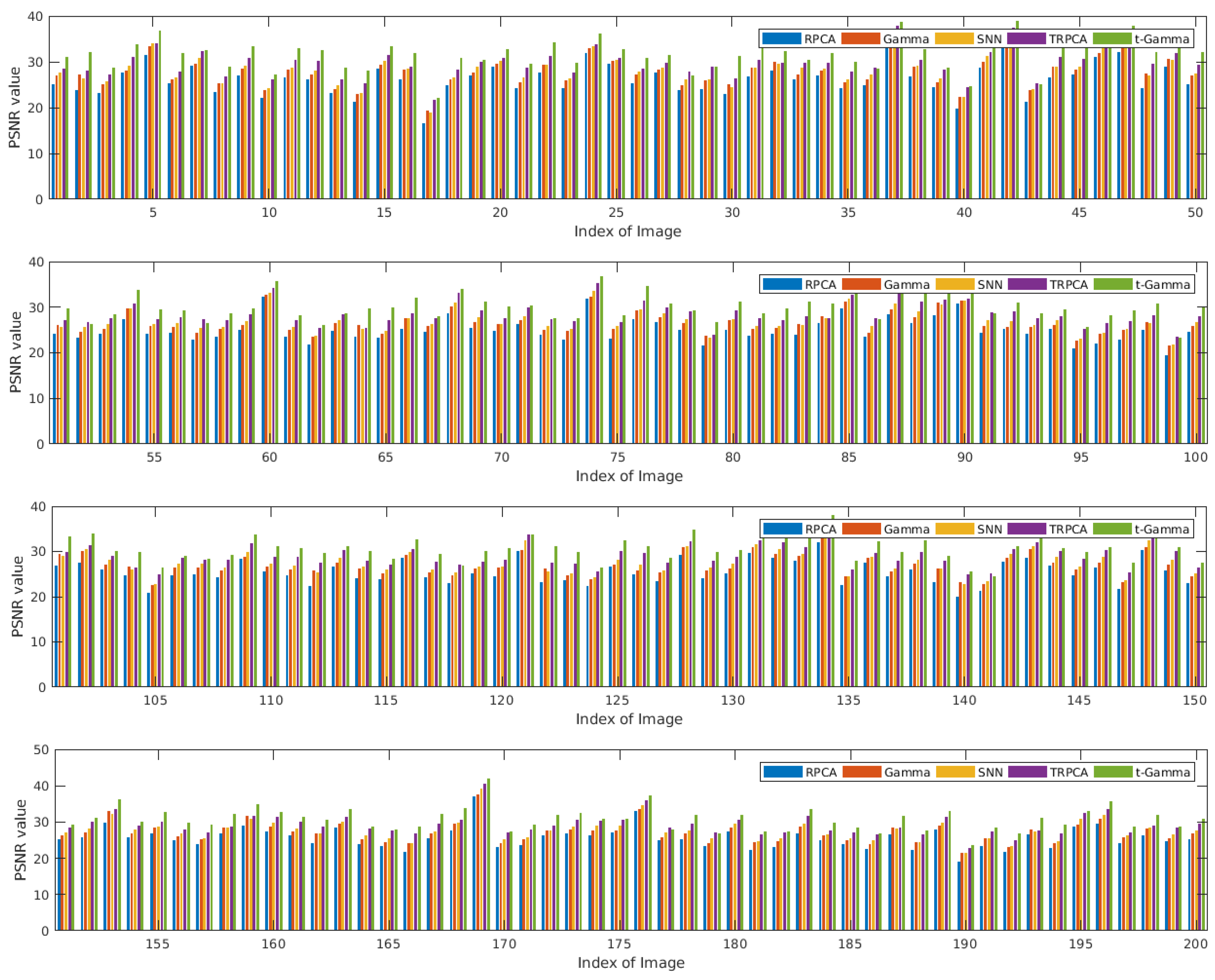
We perform the experiments on Berkeley Segmentation Dataset [48], which contains 200 color image for training. For each image, we randomly set $10\%$ of pixels to the random values in [0, 255], that is, we corrupt the image on 3 channels simultaneously which is more challenging than make corruptions on only one channel. We compare our t-Gamma algorithms with RPCA [4], Gamma [26], SNN [49] and TRPCA [20], in which RPCA minimizes a weighted combination of the nuclear norm and of the $l_1$ norm in matrix form, Gamma replaces the nuclear norm by matrix Gamma quasi-norm, SNN uses the sum of the nuclear norm for all mode-i matricization of the given tensor, and TRPCA extends the RPCA from the matrix to tensor case. For RPCA and Gamma, we conduct the algorithms on each channel, i.e., regarding each channel of the image as a matrix, and then combine the channel recovery result into a color image. The parameter $\lambda$ in RPCA and Gamma is set to $\lambda =\frac{1}{\sqrt{max\{N_1,N_2\}}}$ as suggested in [4]. However, when the parameter $\gamma$ in Gamma is set to $0.01$ as stated in [26], it cannot perform well. We empirically set the $\gamma =\sqrt{min\{N_1,N_2\}}$ in Gamma and t-Gamma. For SNN, we set $\lambda =[15,15,1.5]$ as suggested in [20]. The parameters $\lambda$ in TRPCA and t-Gamma is set to $\lambda =\frac{1}{\sqrt{max\{N_1,N_2\}{N}_3}}$. By using the Peak Signal to Noise Ratio (PSNR) to evaluate the recovery results and PSNR is defined as

$$PSNR=10{log}_{10}\left(\frac{{\parallel \mathcal{M}\parallel }_{\infty }^2}{\frac{1}{N_1{N}_2{N}_3}{\parallel \widehat{\mathcal{X}}-\mathcal{M}\parallel }_F^2}\right).$$

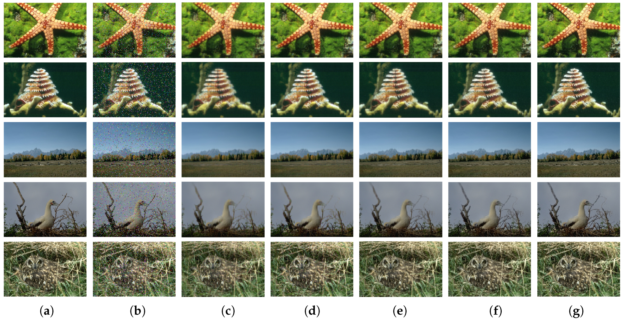
In Figure 1, we give the comparison of PSNR value on 200 images and each subfigure contains 50 results. The sample recovery performance are shown in Figure 2. From Figure 1, we can observe that the proposed t-Gamma algorithm perform better on almost every image and can achieve around 2 dB improvement in many cases.

Table 1. Average PSNR obtained by five Algorithms on 200 images.

Algorithm	RPCA	Gamma	SNN	TRPCA	t-Gamma
Average PSNR	25.5843	27.0762	27.6329	29.1157	30.7896

shows the average recovery performance obtained by these five algorithms on Berkeley Segmentation Dataset. In Figure 2 we can visually conclude that our algorithm yields a better result than the compare algorithms which can illustrate the merit of the our approach.

5.2. Video Background Modeling

5.2.1. Qualitative Experiments

In this part, we consider the background modeling problem, an essential task in video surveillance, which aims to separate the foreground objects from the background. The frames of background in video surveillance are highly correlated and thus it is reasonable to consider it as a low rank tensor. While the objects in the foreground usually only occupy a small part of the image in some frames and hence can regard it as the sparse part.

To solve this problem, we test our algorithm on four example color videos, Hall, MovedObject, Escalator and Lobby http://perception.i2r.a-star.edu.sg/bk_model/bk_index.html, and compare it with RPCA [4], Gamma [26], SNN [49] and TRPCA [20]. We extract $N_2=200$ frames from these four videos. Suppose the size of frames in the given video is $h\times w$, we stack each frame in each color channel as a column vector of size $N_1\times 1$, where $N_1=h\times w$, and then all column vectors into a matrix of size $3N_1\times N_2$ for RPCA and Gamma, and into a tensor of size $N_1\times N_2\times 3$ for SNN, TRPCA and t-Gamma. The parameter $lambda$ is set to $\lambda =\frac{1}{max\{3N_1,N_2\}}$ for RPCA and Gamma, and $\lambda =\frac{1}{max\{N_1,N_2\}3}$ for SNN, TRPCA and t-Gamma. The parameter $\gamma$ in Gamma and t-Gamma is set to $\gamma =\frac{1}{\sqrt{min\{3N_1,N_2\}}}$ and $\gamma =\frac{3}{\sqrt{min\{N_1,N_2\}}}$ respectively. As suggested in [20], $\lambda$ in SNN is set to $[200,2,20]$.

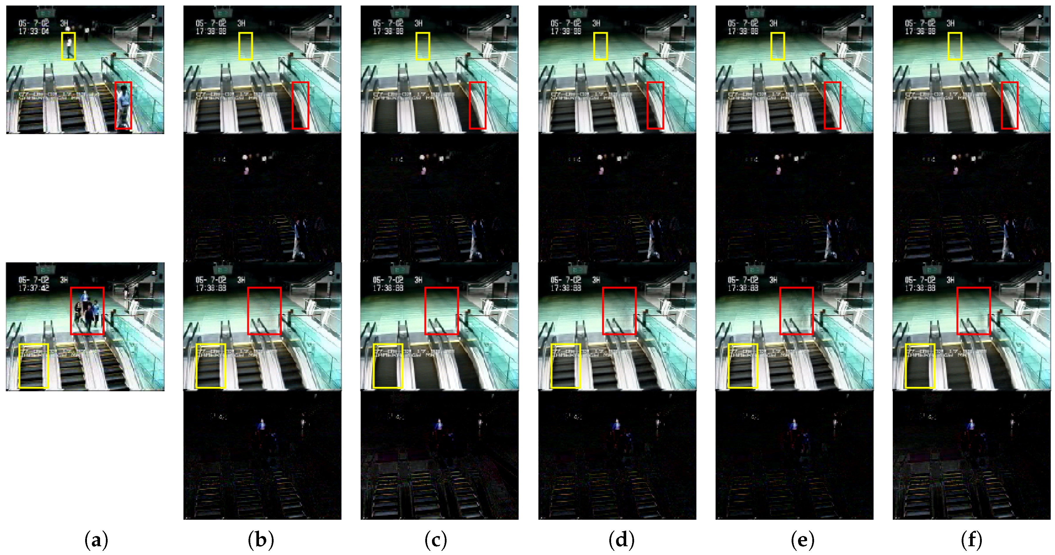
The background separated results are depicted in Figure 3, Figure 4, Figure 5 and Figure 6. In Figure 3 and Figure 4, we can see that our method could reconstruct the background with fewer ghosting effects and more completely. From Figure 5 and Figure 6, it could be observed that though all the method separate the background from the foreground effectively, the proposed algorithm are more robust to the dynamic foreground and illumination variation, e.g., only Gamma and t-Gamma can remove the steps of moving escalator in Figure 5, while the method Gamma cannot adapt to change of illumination in Figure 6.

5.2.2. Quantitative Experiments

Since the datasets in Section 5.2.1 do not include the ground truth background for each frame of the video, we perform the algorithms on the ChangeDetection.net(CDNet) dataset2014 [50] which consists of visual surveillance and smart environments. However, only part of frames are accompanied with ground truth background and thus we only take out some of frames of the video for testing. That is, we select the frames from 900 to 1000 of the dataset highway, pedestrians and PETS2006 in the baseline category. Hence the size of the video will be $h\times w\times 101$, where $h\times w$ is the resolution of each frame, and 101 is the number of frames. We compare our algorithm with RPCA [4], Gamma [26], SNN [49] and TRPCA [20]. The parameters setting is conducted from Section 5.2.1.

To evaluate the performance of the experiment results, we use the three metrics for the quantitative measure, that is, Recall, Precision and F-Measure. They are defined as:

$$\mathrm{Recall}=\frac{\mathrm{TP}}{\mathrm{TP}+\mathrm{FN}},$$

$$\mathrm{Precision}=\frac{\mathrm{TP}}{\mathrm{TP}+\mathrm{FP}},$$

$$\text{F-Measure}=2\frac{\mathrm{Precision}·\mathrm{Recall}}{\mathrm{Precision}+\mathrm{Recall}},$$

where TP, FP and FN are true positives numbers, false positives numbers and false negatives numbers respectively. We primarily use F-Measure for overall evaluation since it combines the metrics Recall and Precision and also makes a balance between Recall and Precision which can be viewed as a good indicators for comparison.

From

Table 2. Quantitative Evaluation for algorithm on CDNet Datasets

Dataset	RPCA			Gamma			SNN			TNN			t-Gamma
	Recall	Precision	F-Measure	Recall	Precision	F-Measure	Recall	Precision	F-Measure	Recall	Precision	F-Measure	Recall	Precision	F-Measure
highway	0.8642	0.9109	0.8869	0.8837	0.9067	0.895	0.6982	0.9041	0.7879	0.8235	0.902	0.861	0.8835	0.909	0.8961
pedestrians	0.9983	0.9419	0.9692	0.9982	0.9275	0.9616	0.9955	0.9285	0.9608	0.9983	0.9258	0.9607	0.9982	0.9309	0.9634
PETS2006	0.8151	0.7131	0.7607	0.8326	0.7678	0.7989	0.288	0.6974	0.4077	0.8033	0.6853	0.7396	0.8301	0.7805	0.8045

, we can see that the proposed algorithm achieves better segmentation performance among the compare methods with respect to the F-Measure. Some of the frames of the segmentation results are shown in Figure 7, it can be observed that among the three dataset in CDNet our method can usually get the clearer and more accurate background segmentation. These quantitative comparison illustrates the superior of t-Gamma tensor quasi-norm as the surrogate of the rank of tensor.

6. Concluding Remarks

In this paper, we conduct the TRPCA with a new t-Gamma tensor quasi-norm used as the regularization for tensor rank function. The t-Gamma tensor quasi-norm is developed via t-SVD in the Fourier domain, which simplifies the required optimization process. Compared with the convex tensor nuclear norm, our regularization approach appears to be more effective in approximating the tensor tubal rank. We incorporate the alternating direction method of multipliers with the t-Gamma tensor quasi-norm to efficiently solve the non-convex TRPCA problem, yielding an approachable framework for non-convex optimization. Numerical experimental results indicate that our approach outperforms the existing methods in distinguishable ways.

References

- Landsberg, J. Tensors: Geometry and Applications; Graduate Studies in Mathematics; American Mathematical Society: Providence, RI, USA, 2012. [Google Scholar]
- Bro, R. Multi-Way Analysis in the Food Industry: Models, Algorithms, and Applications. Ph.D. Thesis, University of Amsterdam (NL), Amsterdam, The Netherlands, 1998. [Google Scholar]
- Yang, M.; Li, W.; Xiao, M. On identifiability of higher order block term tensor decompositions of rank Lr⊗ rank-1. Linear Multilinear Algebra 2018, 1–23. [Google Scholar] [CrossRef]
- Candès, E.J.; Li, X.; Ma, Y.; Wright, J. Robust principal component analysis? J. ACM 2011, 58, 11. [Google Scholar] [CrossRef]
- Wright, J.; Ganesh, A.; Rao, S.; Peng, Y.; Ma, Y. Robust principal component analysis: Exact recovery of corrupted low-rank matrices via convex optimization. In Proceedings of the Advances in Neural Information Processing Systems, Vancouver, BC, USA, 7–10 December 2009; pp. 2080–2088. [Google Scholar]
- Kang, Z.; Pan, H.; Hoi, S.C.H.; Xu, Z. Robust Graph Learning From Noisy Data. IEEE Trans. Cybern. 2019, 1–11. [Google Scholar] [CrossRef]
- Peng, C.; Kang, Z.; Cai, S.; Cheng, Q. Integrate and Conquer: Double-Sided Two-Dimensional k-Means Via Integrating of Projection and Manifold Construction. ACM Trans. Intell. Syst. Technol. 2018, 9, 57. [Google Scholar] [CrossRef]
- Sun, P.; Qin, J. Speech enhancement via two-stage dual tree complex wavelet packet transform with a speech presence probability estimator. J. Acoust. Soc. Am. 2017, 141, 808–817. [Google Scholar] [CrossRef] [PubMed]
- Vaswani, N.; Bouwmans, T.; Javed, S.; Narayanamurthy, P. Robust subspace learning: Robust PCA, robust subspace tracking, and robust subspace recovery. IEEE Signal Process. Mag. 2018, 35, 32–55. [Google Scholar] [CrossRef]
- Bouwmans, T.; Zahzah, E.H. Robust PCA via principal component pursuit: A review for a comparative evaluation in video surveillance. Comput. Vis. Image Underst. 2014, 122, 22–34. [Google Scholar] [CrossRef]
- Bouwmans, T.; Javed, S.; Zhang, H.; Lin, Z.; Otazo, R. On the applications of robust PCA in image and video processing. Proc. IEEE 2018, 106, 1427–1457. [Google Scholar] [CrossRef]
- Cichocki, A.; Lee, N.; Oseledets, I.; Phan, A.H.; Zhao, Q.; Mandic, D.P. Tensor networks for dimensionality reduction and large-scale optimization: Part 1 low-rank tensor decompositions. Found. Trends® Mach. Learn. 2016, 9, 249–429. [Google Scholar] [CrossRef]
- Kilmer, M.E.; Martin, C.D. Factorization strategies for third-order tensors. Linear Algebra Appl. 2011, 435, 641–658. [Google Scholar] [CrossRef]
- Hao, N.; Kilmer, M.E.; Braman, K.; Hoover, R.C. Facial recognition using tensor-tensor decompositions. SIAM J. Imaging Sci. 2013, 6, 437–463. [Google Scholar] [CrossRef]
- Zhang, Z.; Ely, G.; Aeron, S.; Hao, N.; Kilmer, M. Novel methods for multilinear data completion and de-noising based on tensor-SVD. In Proceedings of the IEEE Conference on Computer Vision and Pattern Recognition, Columbus, OH, USA, 23–28 June 2014; pp. 3842–3849. [Google Scholar]
- Signoretto, M.; De Lathauwer, L.; Suykens, J.A. Nuclear norms for tensors and their use for convex multilinear estimation. Linear Algebra Appl. 2010, 43. Available online: ftp://ftp.esat.kuleuven.be/sista/signoretto/Signoretto_nucTensors2.pdf (accessed on 3 April 2019).
- Cichocki, A. Era of big data processing: A new approach via tensor networks and tensor decompositions. arXiv, 2014; arXiv:1403.2048. [Google Scholar]
- Grasedyck, L.; Kressner, D.; Tobler, C. A literature survey of low-rank tensor approximation techniques. GAMM-Mitteilungen 2013, 36, 53–78. [Google Scholar] [CrossRef]
- Lu, C.; Feng, J.; Chen, Y.; Liu, W.; Lin, Z.; Yan, S. Tensor Robust Principal Component Analysis: Exact Recovery of Corrupted Low-Rank Tensors via Convex Optimization. In Proceedings of the 2016 IEEE Conference on Computer Vision and Pattern Recognition (CVPR), Las Vegas, NV, USA, 27–30 June 2016; pp. 5249–5257. [Google Scholar]
- Lu, C.; Feng, J.; Chen, Y.; Liu, W.; Lin, Z.; Yan, S. Tensor Robust Principal Component Analysis with A New Tensor Nuclear Norm. arXiv, 2018; arXiv:1804.03728. [Google Scholar] [CrossRef] [PubMed]
- Semerci, O.; Hao, N.; Kilmer, M.E.; Miller, E.L. Tensor-based formulation and nuclear norm regularization for multienergy computed tomography. IEEE Trans. Image Process. 2014, 23, 1678–1693. [Google Scholar] [CrossRef]
- Ciccone, V.; Ferrante, A.; Zorzi, M. Robust identification of “sparse plus low-rank” graphical models: An optimization approach. In Proceedings of the 2018 IEEE Conference on Decision and Control (CDC), Miami Beach, FL, USA, 17–19 December 2018; pp. 2241–2246. [Google Scholar]
- Ciccone, V.; Ferrante, A.; Zorzi, M. Factor Models with Real Data: A Robust Estimation of the Number of Factors. IEEE Trans. Autom. Control 2018. [Google Scholar] [CrossRef]
- Fazel, S.M. Matrix Rank Minimization with Applications. Ph.D. Thesis, Stanford University, Stanford, CA, USA, 2003. [Google Scholar]
- Recht, B.; Fazel, M.; Parrilo, P.A. Guaranteed minimum-rank solutions of linear matrix equations via nuclear norm minimization. SIAM Rev. 2010, 52, 471–501. [Google Scholar] [CrossRef]
- Kang, Z.; Peng, C.; Cheng, Q. Robust PCA Via Nonconvex Rank Approximation. In Proceedings of the 2015 IEEE International Conference on Data Mining (ICDM), Atlantic City, NJ, USA, 14–17 November 2015; pp. 211–220. [Google Scholar]
- Lewis, A.S.; Sendov, H.S. Nonsmooth analysis of singular values. Part I: Theory. Set-Valued Anal. 2005, 13, 213–241. [Google Scholar] [CrossRef]
- Liu, Y.; Chen, L.; Zhu, C. Improved Robust Tensor Principal Component Analysis via Low-Rank Core Matrix. IEEE J. Sel. Top. Signal Process. 2018, 12, 1378–1389. [Google Scholar] [CrossRef]
- Chen, Y.; Wang, S.; Zhou, Y. Tensor Nuclear Norm-Based Low-Rank Approximation With Total Variation Regularization. IEEE J. Sel. Top. Signal Process. 2018, 12, 1364–1377. [Google Scholar] [CrossRef]
- Kong, H.; Xie, X.; Lin, Z. t-Schatten-p Norm for Low-Rank Tensor Recovery. IEEE J. Sel. Top. Signal Process. 2018, 12, 1405–1419. [Google Scholar] [CrossRef]
- Tarzanagh, D.A.; Michailidis, G. Fast Monte Carlo Algorithms for Tensor Operations. arXiv, 2017; arXiv:1704.04362. [Google Scholar]
- Driggs, D.; Becker, S.; Boyd-Graber, J. Tensor Robust Principal Component Analysis: Better recovery with atomic norm regularization. arXiv, 2019; arXiv:1901.10991. [Google Scholar]
- Sobral, A.; Baker, C.G.; Bouwmans, T.; Zahzah, E.H. Incremental and multi-feature tensor subspace learning applied for background modeling and subtraction. In Proceedings of the International Conference Image Analysis and Recognition, Vilamoura, Portugal, 22–24 October 2014; pp. 94–103. [Google Scholar]
- Sobral, A.; Javed, S.; Ki Jung, S.; Bouwmans, T.; Zahzah, E.H. Online stochastic tensor decomposition for background subtraction in multispectral video sequences. In Proceedings of the IEEE International Conference on Computer Vision Workshops, Santiago, Chile, 7–13 December 2015; pp. 106–113. [Google Scholar]
- Bouwmans, T.; Sobral, A.; Javed, S.; Jung, S.K.; Zahzah, E.H. Decomposition into low-rank plus additive matrices for background/foreground separation: A review for a comparative evaluation with a large-scale dataset. Comput. Sci. Rev. 2017, 23, 1–71. [Google Scholar] [CrossRef]
- Boyd, S.; Parikh, N.; Chu, E.; Peleato, B.; Eckstein, J. Distributed optimization and statistical learning via the alternating direction method of multipliers. Found. Trends® Mach. Learn. 2011, 3, 1–122. [Google Scholar] [CrossRef]
- Kilmer, M.E.; Braman, K.; Hao, N.; Hoover, R.C. Third-order tensors as operators on matrices: A theoretical and computational framework with applications in imaging. SIAM J. Matrix Anal. Appl. 2013, 34, 148–172. [Google Scholar] [CrossRef]
- Tyrtyshnikov, E.E. A Brief Introduction to Numerical Analysis; Springer Science & Business Media: New York, NY, USA, 2012. [Google Scholar]
- Marc Peter Deisenroth, A.A.F.; Ong, C.S. Mathematics for Machine Learning; Cambridge University Press: Cambridge, UK, 2019. [Google Scholar]
- Moreau, J.J. Proximité et dualité dans un espace hilbertien. Bull. Soc. Math. France 1965, 93, 273–299. [Google Scholar] [CrossRef]
- Dong, W.; Shi, G.; Li, X.; Ma, Y.; Huang, F. Compressive Sensing via Nonlocal Low-Rank Regularization. IEEE Trans. Image Process. 2014, 23, 3618–3632. [Google Scholar] [CrossRef] [PubMed]
- Zhang, G.; Lin, Y. Lectures in Functional Analysis; Peking University Press: Beijing, China, 1987. [Google Scholar]
- Donoho, D.L. De-noising by soft-thresholding. IEEE Trans. Inf. Theory 1995, 41, 613–627. [Google Scholar] [CrossRef]
- Lu, H.; Plataniotis, K.; Venetsanopoulos, A. Multilinear Subspace Learning: Dimensionality Reduction of Multidimensional Data; Chapman & Hall/CRC Machine Learning & Pattern Recognition Series; CRC Press: Boca Raton, FL, USA, 2013. [Google Scholar]
- Zhang, Z.; Aeron, S. Exact Tensor Completion Using t-SVD. IEEE Trans. Signal Process. 2017, 65, 1511–1526. [Google Scholar] [CrossRef]
- Luenberger, D.G. Optimization by Vector Space Methods; John Wiley & Sons: New York, NY, USA, 1997. [Google Scholar]
- Liu, J.; Musialski, P.; Wonka, P.; Ye, J. Tensor Completion for Estimating Missing Values in Visual Data. IEEE Trans. Pattern Anal. Mach. Intell. 2013, 35, 208–220. [Google Scholar] [CrossRef] [PubMed]
- Martin, D.; Fowlkes, C.; Tal, D.; Malik, J. A database of human segmented natural images and its application to evaluating segmentation algorithms and measuring ecological statistics. In Proceedings of the Eighth IEEE International Conference on Computer Vision ( ICCV 2001), Vancouver, BC, Canada, 7–14 July 2001; Volume 2, pp. 416–423. [Google Scholar]
- Huang, B.; Mu, C.; Goldfarb, D.; Wright, J. Provable models for robust low-rank tensor completion. Pac. J. Optim. 2015, 11, 339–364. [Google Scholar]
- Goyette, N.; Jodoin, P.-M.; Porikli, F.; Konrad, J.; Ishwar, P. Changedetection.net: A new change detection benchmark dataset, 2012. In Proceedings of the IEEE Workshop on Change Detection (CDW-2012) at CVPR-2012, Providence, RI, USA, 16–21 June 2012. [Google Scholar]
Figure 1.
Comparison of the PSNR values with RPCA [4], Gamma [26], SNN [49], TRPCA [20] and t-Gamma.
Figure 2.
Recovery results on 5 sample images. The first two columns are original and corrupted images reps. The third to seventh columns are recovery images obtained by RPCA, Gamma, SNN, TRPCA and t-Gamma resp. (a) Original; (b) Corrupted; (c) RPCA [4]; (d) Gamma [26]; (e) SNN [49]; (f) TRPCA [20]; (g) t-Gamma.
Figure 3.
Background modeling: two example frames from Hall sequences are shown. (a) Original; (b) RPCA [4]; (c) Gamma [26]; (d) SNN [49]; (e) TRPCA [20]; (f) t-Gamma.
Figure 4.
Background modeling: two example frames from MovedObject sequences are shown. (a) Original; (b) RPCA [4]; (c) Gamma [26]; (d) SNN [49]; (e) TRPCA [20]; (f) t-Gamma.
Figure 5.
Background modeling: two example frames from Escalator sequences are shown. (a) Original; (b) RPCA [4]; (c) Gamma [26]; (d) SNN [49]; (e) TRPCA [20]; (f) t-Gamma.
Figure 6.
Background modeling: two example frames from Lobby sequences are shown. (a) Original; (b) RPCA [4]; (c) Gamma [26]; (d) SNN [49]; (e) TRPCA [20]; (f) t-Gamma.
Figure 7.
Visual results for CDNet dataset. Row 1 and row 2 are samples of highway; row 3 and row 4 are samples of pedestrians; row 5 and row 6 are samples of PETS2006. (a) Original; (b) Ground True; (c) RPCA [4]; (d) Gamma [26]; (e) SNN [49]; (f) TRPCA [20]; (g) t-Gamma