Dynamics of a Partially Confined, Vertical Upward-Fluid-Conveying, Slender Cantilever Pipe with Reverse External Flow

 , ,
, ,
Abstract
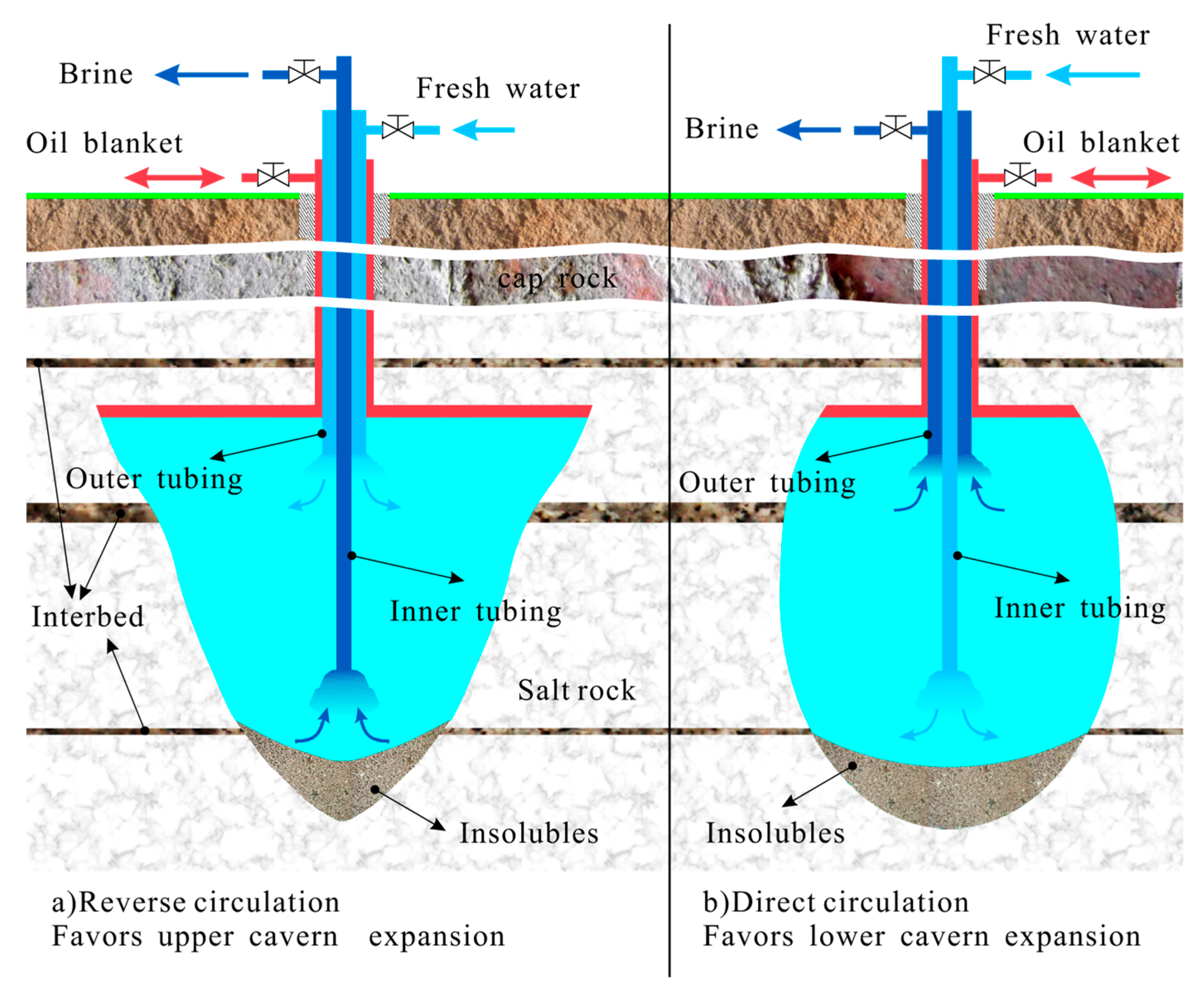
:1. Introduction
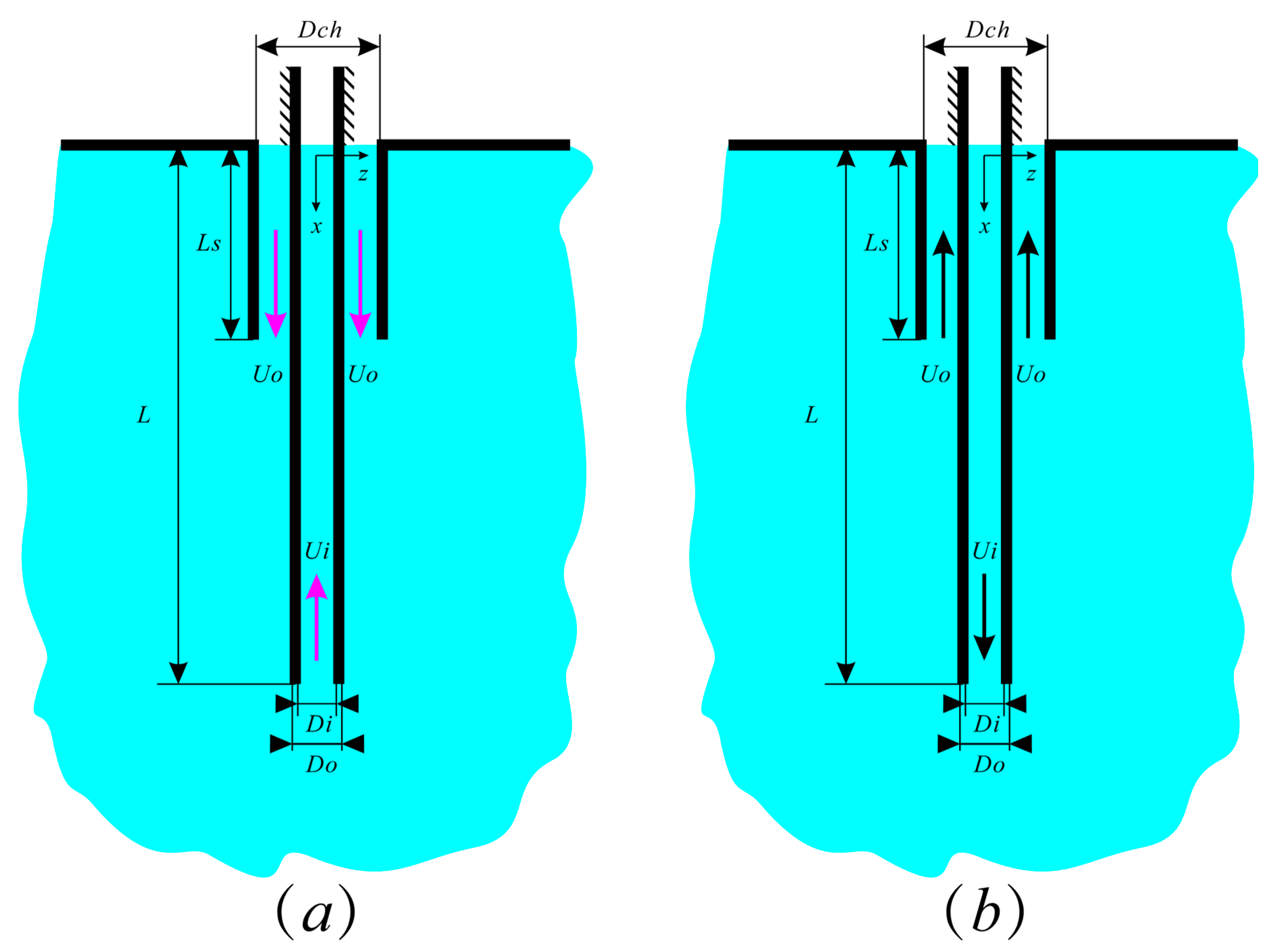
2. Problem Formulation
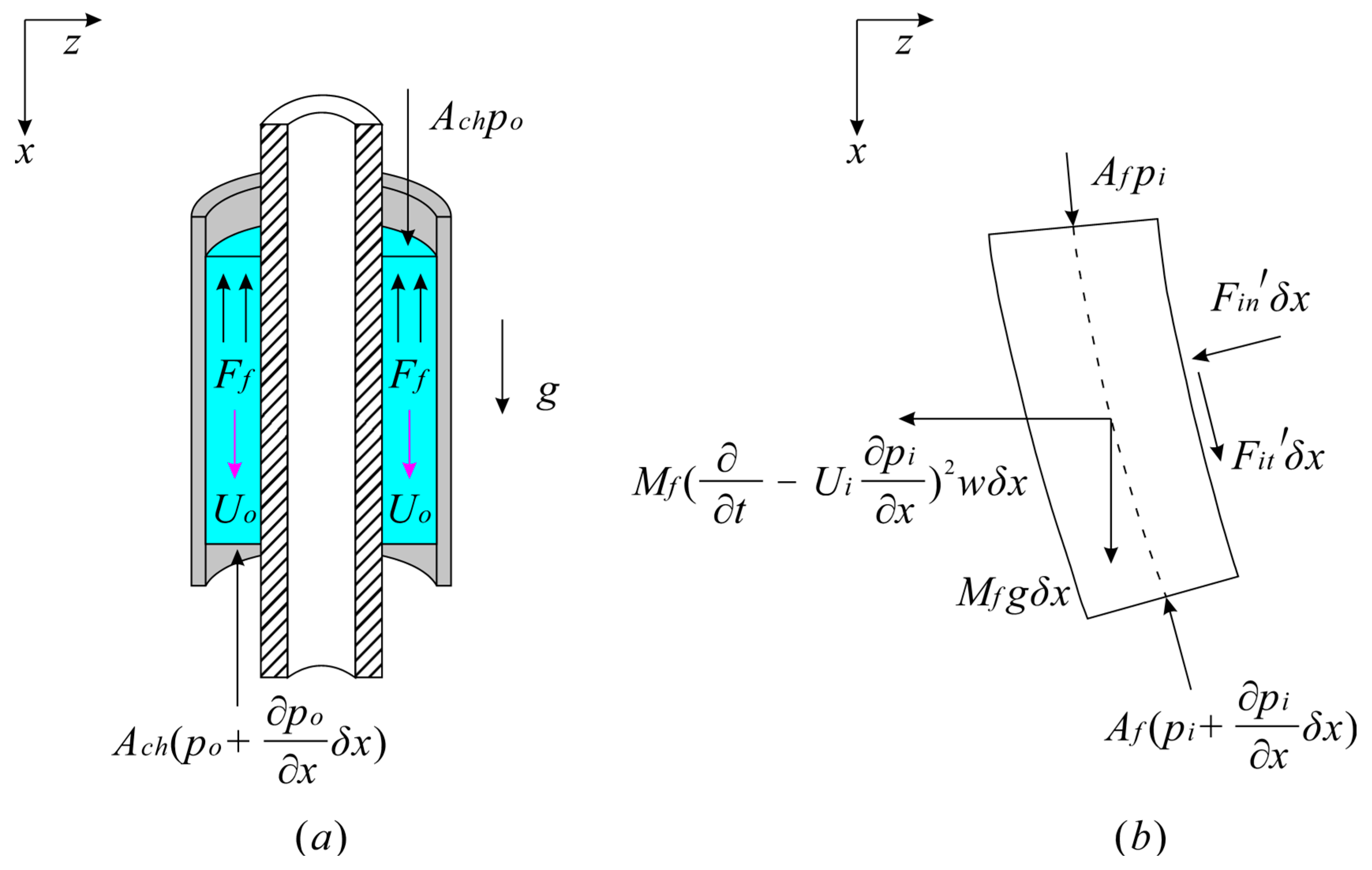
2.1. Derivation of the Motion Equation of Theoretical Model
2.2. Boundary Conditions
2.3. Dimensionless Motion Equation and Boundary Conditions
3. Solution of Equations by a Galerkin Method
4. Theoretical Analysis for Slender, Leaching-Tubing-Like Systems
4.1. Effect of the Radial Confinement αch
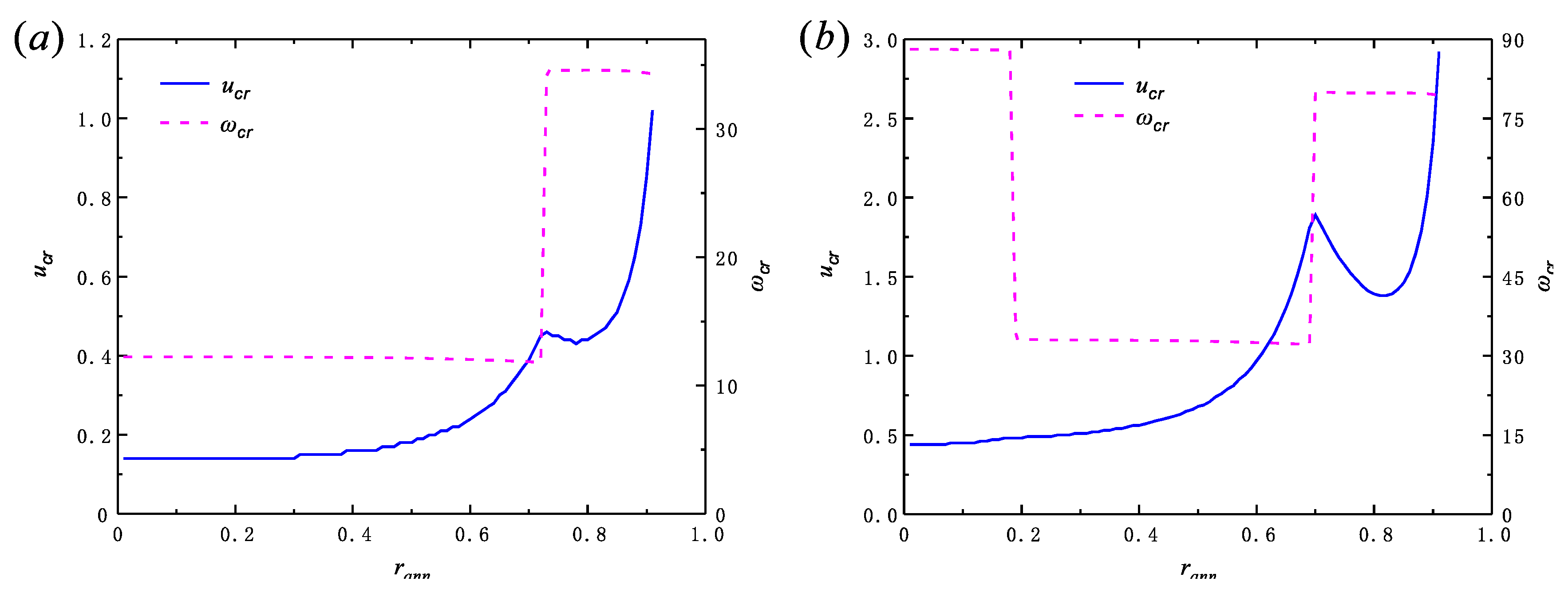
4.2. Effect of the Confinement Length rann
4.3. Effect of the Cantilevered Pipe Length L
5. Conclusions
Author Contributions
Funding
Acknowledgments
Conflicts of Interest
References
- Moditis, K.; Païdoussis, M.P.; Ratigan, J. Dynamics of a partially confined, discharging, cantilever pipe with reverse external flow. J. Fluids Struct. 2016, 63, 120–139. [Google Scholar] [CrossRef]
- Ratigan, J.L. Brine string integrity and model evaluation. In Proceedings of the Processes of SMRI Fall Meeting, Galveston, TX, USA, 13–14 October 2008; pp. 273–293. [Google Scholar]
- Li, Y.; Yang, C.; Qu, D.; Yang, C.; Shi, X. Preliminary study of dynamic characteristics of tubing string for solution mining of oil/gas storage salt caverns. Rock Soil Mech. 2012, 33, 681–686. [Google Scholar]
- Cesari, F.; Curioni, S. Buckling instability in tubes subject to internal and external axial fluid flow. In Proceedings of the 4th Conference on Dimensioning, Hungarian Academy of Science, Budapest, Hungary, October 1971; pp. 301–311. [Google Scholar]
- Hannoyer, M.; Païdoussis, M.P. Instabilities of tubular beams simultaneously subjected to internal and external axial flows. J. Mech. Des. 1978, 100, 328–336. [Google Scholar] [CrossRef]
- Paidoussis, M.P.; Besancon, P. Dynamics of arrays of cylinders with internal and external axial flow. J. Sound Vib. 1981, 76, 361–379. [Google Scholar] [CrossRef]
- Wang, X.; Bloom, F. Dynamics of a submerged and inclined concentric pipe system with internal and external flows. J. Fluids Struct. 1999, 13, 443–460. [Google Scholar] [CrossRef]
- Païdoussis, M.P.; Luu, T.; Prabhakar, S. Dynamics of a long tubular cantilever conveying fluid downwards, which then flows upwards around the cantilever as a confined annular flow. J. Fluids Struct. 2008, 24, 111–128. [Google Scholar] [CrossRef]
- Doaré, O.; De Langre, E. The flow-induced instability of long hanging pipes. Eur. J. Mech. A. Solids 2002, 21, 857–867. [Google Scholar] [CrossRef]
- Lemaitre, C.; Hémon, P.; De Langre, E. Instability of a long ribbon hanging in axial air flow. J. Fluids Struct. 2005, 20, 913–925. [Google Scholar] [CrossRef]
- Kuiper, G.; Metrikine, A. Dynamic stability of a submerged, free-hanging riser conveying fluid. J. Sound Vib. 2005, 280, 1051–1065. [Google Scholar] [CrossRef]
- Kuiper, G.; Metrikine, A. Experimental investigation of dynamic stability of a cantilever pipe aspirating fluid. J. Fluids Struct. 2008, 24, 541–558. [Google Scholar] [CrossRef]
- Chen, S.; Wambsganss, M.T.; Jendrzejczyk, J. Added mass and damping of a vibrating rod in confined viscous fluids. J. Appl. Mech. 1976, 43, 325–329. [Google Scholar] [CrossRef]
- Païdoussis, M.P. Fluid-Structure Interactions: Slender Structures and Axial Flow, 2nd ed.; Academic Press: Oxford, UK, 2014; Volume 1. [Google Scholar]
- Païdoussis, M.P. Fluid-Structure Interactions: Slender Structures and Axial Flow, 2nd ed.; Academic Press: Oxford, UK, 2016; Volume 2. [Google Scholar]
- Lighthill, M. Note on the swimming of slender fish. J. Fluid Mech. 1960, 9, 305–317. [Google Scholar] [CrossRef]
- Paidoussis, M.P. Dynamics of cylindrical structures subjected to axial flow. J. Sound Vib. 1973, 29, 365–385. [Google Scholar] [CrossRef]
- Sinyavskii, V.; Fedotovskii, V.; Kukhtin, A. Oscillation of a cylinder in a viscous liquid. Sov. Appl. Mech. 1980, 16, 46–50. [Google Scholar] [CrossRef]
- Brater, E.F.; King, H.W.; Lindell, J.E.; Wei, C.Y. Handbook of Hydraulics for the Solution of Hydraulic Engineering Problems; McGraw-Hill: Boston, MA, USA, 1996. [Google Scholar]
- Liu, W.; Muhammad, N.; Chen, J.; Spiers, C.; Peach, C.; Deyi, J.; Li, Y. Investigation on the permeability characteristics of bedded salt rocks and the tightness of natural gas caverns in such formations. J. Nat. Gas Sci. Eng. 2016, 35, 468–482. [Google Scholar] [CrossRef]
- Liu, W.; Chen, J.; Jiang, D.; Shi, X.; Li, Y.; Daemen, J.K.; Yang, C. Tightness and suitability evaluation of abandoned salt caverns served as hydrocarbon energies storage under adverse geological conditions (AGC). Appl. Energy 2016, 178, 703–720. [Google Scholar]
- De Langre, E.; Paidoussis, M.; Doaré, O.; Modarres-Sadeghi, Y. Flutter of long flexible cylinders in axial flow. J. Fluid Mech. 2007, 571, 371–389. [Google Scholar] [CrossRef]
- Ge, X.; Li, Y.; Shi, X.; Chen, X.; Ma, H.; Yang, C.; Shu, C.; Liu, Y. Experimental device for the study of liquid–solid coupled flutter instability of salt cavern leaching tubing. J. Nat. Gas Sci. Eng. 2019, in press. [Google Scholar] [CrossRef]


| Dimensional parameters | Di (m) | Do (m) | Dch (m) | L (m) | Ls (m) | EI (N·m2) | Mp (kg/m) | |
| 0.159 | 0.1778 | 0.298 | 1283 | 1085 | 3.47 × 10⁶ | 38.7 | ||
| Dimensionless parameters | α | αch | ε | βi | βo | h | γ | rann |
| 0.897 | 1.676 | 7216 | 0.239 | 0.297 | 1.479 | 2.019 × 10⁵ | 0.85 |
| Behavior a | ||||||||||
|---|---|---|---|---|---|---|---|---|---|---|
| D1 | F2 | F3 | F1 | F2 | ||||||
| αch | 1.10 | 1.20 | 1.27 | 1.32 | 1.35 | … | 4.46 | … | 20 | … |
| Behavior a | ||||||||||
| F1 | F2 | |||||||||
| rann | 0 | 0.15 | 0.30 | 0.45 | 0.60 | 0.72 | 0.75 | 0.80 | 0.85 | 0.90 |
| Behavior b | ||||||||||
| F2 | F1 | F2 | ||||||||
| rann | 0 | 0.15 | 0.19 | 0.45 | 0.60 | 0.69 | 0.75 | 0.80 | 0.85 | 0.90 |
| Behavior a, b, c | ||||||||||
| F1 | ||||||||||
| L (m) | 5 | 150 | 300 | 450 | 500 | |||||
| Behavior d | F2 | |||||||||
| L (m) | 5 | 150 | 300 | 450 | 500 | |||||
© 2019 by the authors. Licensee MDPI, Basel, Switzerland. This article is an open access article distributed under the terms and conditions of the Creative Commons Attribution (CC BY) license (http://creativecommons.org/licenses/by/4.0/).
Share and Cite
Ge, X.; Li, Y.; Chen, X.; Shi, X.; Ma, H.; Yin, H.; Zhang, N.; Yang, C. Dynamics of a Partially Confined, Vertical Upward-Fluid-Conveying, Slender Cantilever Pipe with Reverse External Flow. Appl. Sci. 2019, 9, 1425. https://doi.org/10.3390/app9071425
Ge X, Li Y, Chen X, Shi X, Ma H, Yin H, Zhang N, Yang C. Dynamics of a Partially Confined, Vertical Upward-Fluid-Conveying, Slender Cantilever Pipe with Reverse External Flow. Applied Sciences. 2019; 9(7):1425. https://doi.org/10.3390/app9071425
Chicago/Turabian StyleGe, Xinbo, Yinping Li, Xiangsheng Chen, Xilin Shi, Hongling Ma, Hongwu Yin, Nan Zhang, and Chunhe Yang. 2019. "Dynamics of a Partially Confined, Vertical Upward-Fluid-Conveying, Slender Cantilever Pipe with Reverse External Flow" Applied Sciences 9, no. 7: 1425. https://doi.org/10.3390/app9071425