Application of a Real-Time Visualization Method of AUVs in Underwater Visual Localization

School of Mechanical Engineering and Automation, Harbin Institute of Technology (Shenzhen), Shenzhen 518055, China
*
Author to whom correspondence should be addressed.
Appl. Sci. 2019, 9(7), 1428; https://doi.org/10.3390/app9071428
Submission received: 4 March 2019
/
Revised: 29 March 2019
/
Accepted: 1 April 2019
/
Published: 4 April 2019
(This article belongs to the Special Issue Intelligent Imaging and Analysis)
Abstract
:Autonomous underwater vehicles (AUVs) are widely used, but it is a tough challenge to guarantee the underwater location accuracy of AUVs. In this paper, a novel method is proposed to improve the accuracy of vision-based localization systems in feature-poor underwater environments. The traditional stereo visual simultaneous localization and mapping (SLAM) algorithm, which relies on the detection of tracking features, is used to estimate the position of the camera and establish a map of the environment. However, it is hard to find enough reliable point features in underwater environments and thus the performance of the algorithm is reduced. A stereo point and line SLAM (PL-SLAM) algorithm for localization, which utilizes point and line information simultaneously, was investigated in this study to resolve the problem. Experiments with an AR-marker (Augmented Reality-marker) were carried out to validate the accuracy and effect of the investigated algorithm.
1. Introduction
Underwater research has been evolving rapidly during the last few decades and autonomous underwater vehicles (AUVs), as an important part of underwater research, are widely used in harsh underwater environments instead of human exploration. However, it is a tough challenge to guarantee the underwater location accuracy of AUVs. Currently, many methods are used to position AUVs, such as inertial measurement units (IMUs), Doppler velocity logs (DVLs), pressure sensors, sonar and visual sensors. For example, Fallon et al. used a side-scan sonar and a forward-look sonar as perception sensors in an AUV for mine countermeasures and localization [1]. The graph was initialized by pose nodes from a GPS, and a nonlinear least square optimization was performed for the dead-reckoning (DVL and IMU) sensor and sonar images. However, sonars are susceptible to interference from the water surface and other sources of sound reflection in shallow water areas. To localize the AUV, inertial units (from an accelerometer or gyroscope), DVLs and pressure sensors are fused by Kalman filter [2]. However, this approach is prone to generating drift without a periodical correction based on a loop closing detection mechanism.
AUVs needs to have good positioning accuracy in shallow water areas, and this paper introduces a periodic correction based on a closed-loop detection mechanism to further improve positioning accuracy. Therefore, the visual simultaneous localization and mapping (SLAM) localization method was chosen in this study. In shallow water areas, visual sensors are better than sonar because they cannot be affected by reflection. The SLAM [3] technique has proved to be one of the most popular and available methods to perform precise localization in unknown environments. When the AUV reaches a position that it has been to before, SLAM provides a loop detection mechanism that eliminates cumulative errors and drift.
Although the quality of the picture will be seriously affected by the scattering and attenuation of underwater light and poor illumination conditions, cameras have larger spatial and temporal resolutions compared to acoustic sensors, which makes cameras more suitable for certain applications, such as surveying, object identification and intervention [4]. Hong and Kim proposed a computationally efficient approach that could be applied in visual simultaneous localization and mapping for the autonomous inspection of underwater structures using monocular vision [5]. Jung et al. proposed a vision-based simultaneous localization and mapping of AUVs in which underwater artificial landmarks were used to help the visual sensing of forward- and downward-looking cameras [6]. Kim and Eustice performed a visual SLAM using monocular video images and utilized a special saliency method using local and global saliency for feature detection in hull inspection [7]. Carrasco et al. proposed the stereo graph-SLAM algorithm for the localization and navigation of underwater vehicles, which optimized the vehicle trajectory and processed the features from the graph [8]. Negre et al. proposed a novel technique to detect loop closings visually in underwater environments to increase the accuracy of vision-based localization systems [9].
All of the above-mentioned visual SLAM methods are based on point feature localization. However, the above methods would cause instability of the system because of the low-texture in many underwater environments, which contain a small number of point features. However, there are rich planar elements in the linear shapes in many low-texture environments, from which line segment features can be extracted. Based on the oriented FAST (Features From Accelerated Segment Test) and rotated brief SLAM (ORB-SLAM) [10] framework, point and line SLAM PL-SLAM [11] can simultaneously utilize point and line information. As suggested in [12], lines are parameterized by their endpoints, the precise locations of which are estimated by following a two-step optimization process in the image plane. In this representation, lines were integrated within the SLAM machinery as if they were points and were hence able to be processed by reusing the ORB-SLAM [10] architecture.
The line segment detector (LSD) method [13] was applied to extract line segments, as it has high precision and repeatability. For stereo matching and frame-to-frame tracking, line segments are augmented with a binary descriptor provided by the line band descriptor (LBD) method [14], which is useful to find correspondences among lines based on their local appearance. The characteristics of LBD were used in the closed-loop detection mechanism outlined below.
In this paper, a visual-based underwater location approach is presented. In Section 2, the PL-SLAM method is presented for real-time underwater localization, including estimation of the real-time position of the AUV, closed loop detection and a closed-loop optimization algorithm based on point-line features. Section 3 is the experimental section, in which the errors of positioning for linear and arbitrary trajectory motions are evaluated. Section 4 summarizes the experimental results and analyzes the problems.
2. Methodology
In the underwater stereo visual localization algorithm, both ORB [10] feature points and LSD [13] line features were selected in this study. The system is composed of three main modules, including tracking, local mapping and loop closing. In the tracking thread, the camera’s position is estimated and the timing of when to add new key-frames is decided. In the local mapping thread, the new key-frame information is added into the map and it is optimized using bundle adjustment (BA). In the loop closing thread, loops are checked and corrected constantly.
2.1. Line Segment Feature Algorithm
Point features are mainly corner points in the image. At present, there are a lot of widely used point feature detection and extraction algorithms such as scale invariant feature transform (SIFT), speeded up robust features (SURF) and oriented FAST and rotated brief (ORB). Compared to other algorithms, ORB has a high extraction speed and good real-time performance while maintaining the invariance of feature sub-rotation and scale. Since it is likely that sufficient point features of the splicing registration algorithm cannot be effectively extracted in underwater environments, the robustness of the algorithm decline. In contrast, line features are mainly the edges of objects in the image. The depth information in the line segment feature changes less and thus the line segment feature is easier to extract underwater. Thus, the robustness of the algorithm is improved.
Line segment detection is an important and frequently used application in computer vision. In the traditional method, the Canny edge detector is used to extract the edge information and then the line segments consisting of edge points exceeding the set threshold are extracted by Hough transform. Finally, the length thresholds are used to select these line segments. There are serious defects in extracting straight lines by Hough transformation, and error detection will occur at a high edge density. In addition, this method has high time complexity and cannot be used as the line segment extraction algorithm for underwater real-time positioning.
As shown in Figure 1, LSD is an extraction algorithm that extracts sub-pixel precision line segments in linear time. It uses heuristic search and inverse verification methods to achieve sub-pixel precision in linear time without setting any parameters. It defines a line segment as the image region, called the line-support region, which is a straight region the points of which have roughly the same image gradient angle. Finally, the judgement as to whether the line-support region is a line segment is conducted by counting the number of aligned points.
2.2. Motion Estimation
After extracting the ORB point features and LSD line segment features, feature matching between continuous frames is carried out by the traditional violent matching method. After the correspondences between two stereo frames are established, the key points and line segments of the first frame is projected to the next frame. In order to estimate the movements, robust Gauss–Newton minimization is used to reduce the error of the line and key-point projections [11].
The difference between the transformed coordinates of the 3D point in the first frame image and in the second frame image is denoted as the re-projection error of the point. It can be solved by Equation (1):
where is the coordinates of the three dimensional points on the second frame, and is the coordinates of the three dimensional points on the first frame. The traditional violent matching method indicates the information that features in frame n and that corresponds to feature in frame n + 1. is the coordinates of the point projected onto the second frame from the first frame image after the transformation of . is the motion transformation matrix between two frames, including rotation and displacement. i is the sequence number of the points feature. The first frame and the second frame are consecutive in time.
The sum of the distances between the two transformed corresponding endpoints of the two frame images is the re-projection error of the line segment (see Figure 2). It can be solved by Equation (2):
where is the corresponding line segment feature on the second frame image, and . and are the coordinates of two endpoints of a line segment feature transformed on the second frame image. and are the coordinates of two endpoints of a line segment feature transformed from the first frame image to the second frame image. is the distance from to . is the distance from to . j is the sequence number of the line segment feature.
For the point-line-feature pairs on the two frames, the pose transformation of two frames can be obtained by minimizing the sum of the re-projection errors. It can be solved by Equation (3):
where is the inverse of the covariance matrix of the point re-projection error. is the inverse of the covariance matrix of the re-projection error of a line.
Although the motion transformation matrix can be obtained according to Equations (1)–(3), it still has some errors because of the mistaken matching of point features and line segment features. Thus we called it an “estimate”. These errors are eliminated in the closed-loop optimization in the following section.
2.3. Closed Loop Detection and Closed-Loop Optimization Algorithm Based on Point-Line Features
Closed loop detection is mainly used to judge whether the AUV is in the area that has been visited before on the basis of the current observation data [9]. If it is in such an area, a complete graph structure is constructed and redundant constraints are added.
The main purpose of the closed loop test is to eliminate the cumulative error caused by inter-frame registration and the basic idea is to compare the current frame with all the key frames in the system. If they are similar, a closed loop is generated. The methods for judging similarity are presented below.
In contrast to the previous closed loop algorithm, or feature dictionary, the characteristic dictionary tree used in this paper is generated by the off-line training of point-line features. The basic training method consists of three steps, as follows.
- A simple K-means clustering method is used to obtain each leaf node at the bottom of the tree structure. Then the nodes of each layer are obtained in turn. Thus the training process of the feature tree can be completed.
- When the new data is collected, the point-line features are extracted first, and the corresponding number of words in the dictionary are obtained using these features. Thus each picture can be described by the vectors, which are composed of the number of words in the characteristic dictionary tree. The vectors are called bags of words vectors (BOWV).
For each word vector in each image, it is important to calculate the distance between two vectors as it is necessary to be able to determine the similarity between the two images. The shorter the distance, the more similar the two images are. A shorter distance also indicates that the AUV may reach the previous positions.
The specific approach is as follows. For the two vectors and definitions, the evaluation scores based on the L1 norm can be defined as follows:
where is the eigenvector of the current frame, and is the eigenvector of the dictionary and the previous frame.
The higher the evaluation score, the greater the similarity between the two images and the greater the possibility of a closed loop. When the above score exceeds the set value, the algorithm enters the closed-loop optimization state.
After estimating all consecutive loop closures in the trajectory, both sides of the loop closure are fused and the error distributed along the loop is corrected. Usually, the pose graph optimization (PGO) method is required in this process. The main purpose of pose graph optimization is to optimize the previous pose of a robot using the redundant constraints. The redundant constraints are obtained by closed-loop detection. When the robot walks to a position where it has walked before, the pose matrix changes due to the accumulation of errors. At this time, the redundant constraint is to reduce the error of the pose matrix. The process can be explained as follows: , which represents the state quantity of the pose matrix of the robot at t moment. Where and is the pose transition matrix between frames k − 1 and k, and are the observed transformation matrix and information matrix (representing the weight of noise) from the state of i time to the state of j time. is a real transformation matrix. The error function is shown in Equation (5).
The sum of the overall error functions is:
The goal of optimization is to find the u that minimizes F(u):
Then a first-order Taylor expansion on the error function is performed:
Then let , , , so we can obtain Formula (9):
In order to find the minimum of Equation (9), we can use the following formula:
Thus,
Through the above formula, the increment of each iteration is calculated using the L-M iterative algorithm. This kind of problem can be optimized through the g2o (General Graph Optimization) library [15], which can greatly simplify the operation.
3. Results
In this section, three experiments were performed, including walking along the wall of a pool, walking along a linear route, and walking along an irregular route. The robustness of the algorithm is verified and the accuracy is evaluated. Finally, a description of the experimental environment and AUV is provided.
3.1. Experiment in an Artificial Pool
An AUV was controlled to walk along the wall of a pool to build an underwater three-dimensional map composed of spatial points and lines (as shown in Figure 4). The AUV performed well with the PL-SLAM method. However, the other visual SLAM algorithms were prone to collapse. The phenomenon of system collapse due to the lack of features was greatly reduced, and the actual frame rate remained at around 20 fps. In order to display the trajectory of the AUV in real time, the pose information was translated into the path topic of the ROS (Robot Operating System). In Figure 5, the color axis represents the AUV’s pose, and the yellow line represents the real time trajectory.
3.2. Comparison of Pose Measurement Experiments with AR-Markers
In order to further verify the accuracy of the underwater algorithm, the algorithm was compared with an AR-marker, because there is no cumulative error and drift in the attitude information measured by an AR-marker. An AR-marker with a length of 150 mm was arranged in the experimental scene, so that the AR-marker always appeared in the field of vision of the AUV. For convenient measurement, the ARToolKitPlus [16] library was used to measure the attitude of the AR-marker. ARToolKitPlus is a software library for calculating camera position and orientation relative to physical markers in real time (see Figure 6)
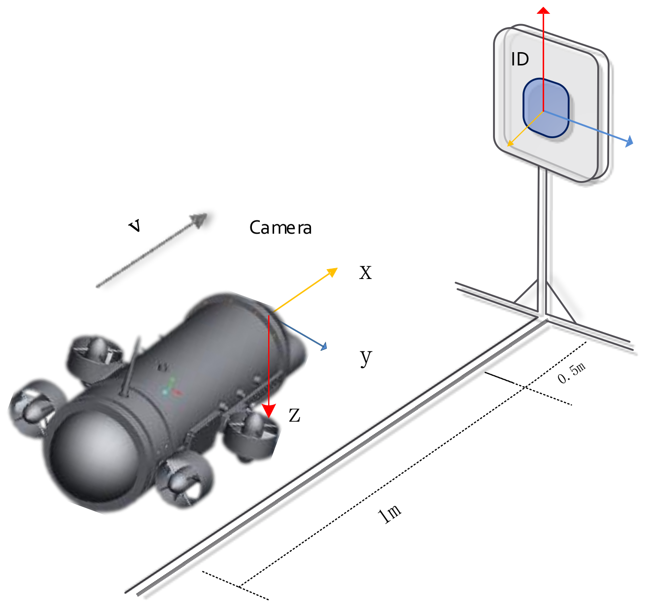
The AUV was set to walk along a linear route. The process of the experiment is shown in Figure 7. The AR-marker recognition program and PL-SLAM were used simultaneously. The straightness of the AUV’s walking trajectory as found using the PL-SLAM was analyzed and the accuracy of the pose measurement using PL-SLAM was compared with the AR-marker. The results of the experiment are shown in Figure 8. The deviation in the y,z-direction was within 5 cm. Because the AUV was not able to be strictly aligned to the center of the y,z-plane, the deviation was within the acceptable range. As shown in Figure 9, the motion trajectories of the two were approximately close, and the final error was less than 3 cm in the x-direction.
As shown in Figure 10, in order to analyze the cumulative error generated by the algorithm, the fixed AR-marker was arranged to appear in view of the camera at the beginning and end of the experiment, as described in Section 3.1. Thus, the accurate termination attitude of the AUV was obtained. After the algorithm finished running, the AUV’s termination attitude with cumulative error was also able to be obtained. These two termination attitudes were compared and the error rates are shown in Table 1.
According to Table 1, the attitude error was . The AUV walked 4.98 m during the experiment described in Section 3.1. Thus, the relative error was 2.98%.
3.3. Experiment Setup
Nvidia Jetson TX2 was chosen as the platform, with an Ubuntu 16.04 system and ROS kinetic. The embedded development board was located in the sealing bin of the AUV. The ZED stereo camera (forward-looking) was located in the head of the AUV. The two parts were connected through the USB (Universal Serial Bus) 3.0 interface (see Figure 13a). The length of the AUV was approximately 730 mm and the diameter of the cabin was approximately 220 mm. Because of the limited experimental conditions, the experiment was only carried out in an artificial pool with a diameter of 4 m and a depth of 1.5 m. Scenes were placed in the pool to simulate the natural environment of the shallow water area (see Figure 13b). In the experiment, the speed of the AUV was set to 0.6 m/s.
Due to the large distortion of the underwater scene, the stereo camera should have been calibrated first. However, camera calibration based on rigorous underwater camera calibration models is time-consuming and cannot achieve real-time performance. Thus, the traditional pinhole model in air was selected to calibrate the AUV. The calibration experiment shows that the refraction effect was considered to be absorbed by the focal length and radial distortion, and the conclusion was that when the camera is in an underwater environment, the focal length is approximately 1.33 times of that in air.
4. Discussion
The experimental results showed that the algorithm was highly robust in underwater low-texture environments due to the inclusion of line segments. At the same time, the algorithm achieved a high accuracy of location effectively, which means that it can be implemented in the navigation and path planning of AUVs in the future. The current positioning accuracy was 2.98%. The experimental environment simulated a shallow water area well, and also verified that the visual positioning method can be applied in shallow water areas. However, there were some problems with the experiment. The added line features undoubtedly increased the complexity of the algorithm, which is more time-consuming than ORB-SLAM. Secondly, it was difficult to calibrate the underwater cameras, especially using the stereo underwater calibration model, however this fact is beyond the scope of our discussion. Due to the fact that high distortion cannot be neglected in underwater environments, the matching of line features occasionally failed. However, the ORB-SLAM algorithm also often fails due to the small number of point features in an underwater environment. The PL-SLAM algorithm combined with the point line feature method had a high success rate. Finally, the accuracy of the pose measured by the AR-marker is not very high and therefore can only be used as a reference.
5. Conclusions
Future work will focus on the following two points: eliminating point features and line features near the edges of the image in a high underwater distortion environment in order to reduce mismatch caused by distortion, and considering matching two stereo cameras, one looking forward and the other looking down, and improving the real-time performance of the algorithm.
Author Contributions
Conceptualization, X.W. and R.W.; methodology, M.Z.; software, R.W.; validation, X.W., R.W. and Y.L.; formal analysis, Y.L.; investigation, M.Z.; resources, Y.L.; data curation, R.W.; writing—original draft preparation, M.Z.; writing—review and editing, R.W.; supervision, X.W.; project administration, X.W.; funding acquisition, X.W.
Funding
This research was funded by the Shenzhen Bureau of Science Technology and Information, grant number No. JCYJ20170413110656460 and grant number No. JCYJ20180306172134024.
Conflicts of Interest
The authors declare no conflict of interest.
References
- Fallon, M.F.; Folkesson, J.; McClelland, H.; Leonard, J.J. Relocating Underwater Features Autonomously Using Sonar-Based SLAM. IEEE J. Ocean. Eng. 2013, 38, 500–513. [Google Scholar] [CrossRef]
- Karimi, M.; Bozorg, M.; Khayatian, A. Localization of an Autonomous Underwater Vehicle using a decentralized fusion architecture. In Proceedings of the 2013 9th Asian Control Conference (ASCC), Istanbul, Turkey, 23–26 June 2013. [Google Scholar]
- Durrant-Whyte, H.; Bailey, T. Simultaneous localization and mapping (SLAM): Part I. IEEE Robot. Autom. Mag. 2006, 13, 99–110. [Google Scholar] [CrossRef]
- Bonin, F.; Burguera, A.; Oliver, G. Imaging systems for advanced underwater vehicles. J. Mariti. Res. 2011, 8, 65–86. [Google Scholar]
- Hong, S.; Kim, J. Selective image registration for efficient visual SLAM on planar surface structures in underwater environment. Auton. Robots 2019, 1–15. [Google Scholar] [CrossRef]
- Jung, J.; Lee, Y.; Kim, D.; Lee, D.; Myung, H.; Choi, H.-T. AUV SLAM using forward/downward looking cameras and artificial landmarks. In Proceedings of the 2017 IEEE Underwater Technology (UT), Busan, Korea, 21–24 February 2017. [Google Scholar]
- Kim, A.; Eustice, R.M.R. Real-Time Visual SLAM for Autonomous Underwater Hull Inspection Using Visual Saliency. IEEE Trans. Robot. 2013, 29, 719–733. [Google Scholar] [CrossRef]
- Carrasco, P.L.N.; Bonin-Font, F.; Codina, G.O. Stereo Graph-SLAM for Autonomous Underwater Vehicles; Intelligent Autonomous Systems 13; Springer International Publishing: Cham, Switzerland, 2016; pp. 351–360. [Google Scholar]
- Negre, P.L.; Bonin-Font, F.; Oliver, G. Cluster-based loop closing detection for underwater slam in feature-poor regions. In Proceedings of the IEEE International Conference on Robotics and Automation, Stockholm, Sweden, 16–21 May 2016; pp. 2589–2595. [Google Scholar]
- Mur-Artal, R.; Montiel, J.M.M.; Tardos, J.D. ORB-SLAM: A versatile and accurate monocular slam system. TRO 2015, 31, 1147–1163. [Google Scholar] [CrossRef]
- Pumarola, A.; Vakhitov, A.; Agudo, A.; Sanfeliu, A.; Moreno-Noguer, F. PL-SLAM: Real-time monocular visual SLAM with points and lines. In Proceedings of the IEEE International Conference on Robotics and Automation, Singapore, 29 May–3 June 2017. [Google Scholar]
- Vakhitov, A.; Funke, J.; Moreno-Noguer, F. Accurate and linear time pose estimation from points and lines. In ECCV 2016; Springer: Cham, Switzerland, 2016. [Google Scholar]
- Von Gioi, R.G.; Jakubowicz, J.; Morel, J.M.; Randall, G. LSD: A line segment detector. IPOL 2012, 2, 35–55. [Google Scholar] [CrossRef]
- Zhang, L.; Koch, R. An efficient and robust line segment matching approach based on LBD descriptor and pairwise geometric consistency. JVCIR 2013, 24, 794–805. [Google Scholar] [CrossRef]
- Kümmerle, R.; Grisetti, G.; Strasdat, H.; Konolige, K.; Burgard, W. G2o: A general framework for graph optimization. In Proceedings of the 2011 IEEE International Conference on Robotics and Automation (ICRA), Shanghai, China, 9–13 May 2011; pp. 3607–3613. [Google Scholar]
- Available online: https://github.com/paroj/artoolkitplus (accessed on 1 June 2018).
Figure 1.
Feature map of underwater extraction lines.

Figure 2.
The re-projection error of the line segments.

Figure 3.
Dictionary tree based on point-line features.

Figure 4.
Stereo PL-SLAM performed in an artificial pool. (a) The green line represents the line features in the global map. The green quadrilateral box represents the current camera. The grey rough line represents the trajectory; (b) The red and black points represent the current local map points and global map points.

Figure 5.
Trajectory of the AUV launched by RVIZ (a 3D visualizer for the Robot Operating System (ROS) framework) released by ROS kinetic.
Figure 5.
Trajectory of the AUV launched by RVIZ (a 3D visualizer for the Robot Operating System (ROS) framework) released by ROS kinetic.

Figure 6.
Comparison of pose measurement experiments with the AR-marker. (a) The red square locking AR-marker indicated that the recognition of the AR-marker was successful, which allows us to obtain the transformation matrix between the camera coordinate system and the AR-marker coordinate system. (b) Using the AR-marker recognition program and PL-SLAM simultaneously.

Figure 7.
The linear motion experiment.

Figure 8.
Results of the linear motion experiments. The experimental diagram is shown in Figure 7. The red curve and the yellow curve indicate that the Z-direction and Y-direction pose changes measured by PL-SLAM were small. The blue curve indicates that the change of the X-direction pose measured by PL-SLAM was proportional to time.

Figure 9.
Result of the linear motion experiments in the X-direction, using the AR-marker recognition program and PL-SLAM simultaneously. The experimental diagram is shown in Figure 7.
Figure 9.
Result of the linear motion experiments in the X-direction, using the AR-marker recognition program and PL-SLAM simultaneously. The experimental diagram is shown in Figure 7.

Figure 10.
Camera vision in the experiment described in Section 3.1. (a) Camera vision at the beginning; (b) Camera vision at the end.
Figure 10.
Camera vision in the experiment described in Section 3.1. (a) Camera vision at the beginning; (b) Camera vision at the end.

Figure 11.
Comparison of the pose measurement experiments with the AR-marker.

Figure 12.
Analysis and contrast diagram of the experimental results. The blue scatter points Pb (Xb, Yb, Zb) represent the PL-SLAM positions. The red scatter points Pr (Xr, Yr, Zr) represent the AR-marker positions.
Figure 12.
Analysis and contrast diagram of the experimental results. The blue scatter points Pb (Xb, Yb, Zb) represent the PL-SLAM positions. The red scatter points Pr (Xr, Yr, Zr) represent the AR-marker positions.

Figure 13.
The developed shark AUV. (a) The appearance of the AUV; (b) Experiment in an artificial pool.
Figure 13.
The developed shark AUV. (a) The appearance of the AUV; (b) Experiment in an artificial pool.


Table 1.
Error comparison of termination attitude.
| Attitude_z (m) | Attitude_y (m) | Attitude_x (m) | Attitude_Error | |
|---|---|---|---|---|
| AR-marker | −0.4523 | 0.1434 | −1.056 | 2.98% |
| PL-SLAM | −0.3651 | 0.2180 | −1.151 | |
| Error | 0.0872 | 0.0746 | −0.095 |
© 2019 by the authors. Licensee MDPI, Basel, Switzerland. This article is an open access article distributed under the terms and conditions of the Creative Commons Attribution (CC BY) license (http://creativecommons.org/licenses/by/4.0/).
Share and Cite
MDPI and ACS Style
Wang, R.; Wang, X.; Zhu, M.; Lin, Y. Application of a Real-Time Visualization Method of AUVs in Underwater Visual Localization. Appl. Sci. 2019, 9, 1428. https://doi.org/10.3390/app9071428
AMA Style
Wang R, Wang X, Zhu M, Lin Y. Application of a Real-Time Visualization Method of AUVs in Underwater Visual Localization. Applied Sciences. 2019; 9(7):1428. https://doi.org/10.3390/app9071428
Chicago/Turabian StyleWang, Ran, Xin Wang, Mingming Zhu, and Yinfu Lin. 2019. "Application of a Real-Time Visualization Method of AUVs in Underwater Visual Localization" Applied Sciences 9, no. 7: 1428. https://doi.org/10.3390/app9071428
Note that from the first issue of 2016, this journal uses article numbers instead of page numbers. See further details here.