Energy-Aware Online Non-Clairvoyant Scheduling Using Speed Scaling with Arbitrary Power Function

Abstract

Efficient job scheduling reduces energy consumption and enhances the performance of machines in data centers and battery-based computing devices. Practically important online non-clairvoyant job scheduling is studied less extensively than other algorithms. In this paper, an online non-clairvoyant scheduling algorithm Highest Scaled Importance First (HSIF) is proposed, where HSIF selects an active job with the highest scaled importance. The objective considered is to minimize the scaled importance based flow time plus energy. The processor’s speed is proportional to the total scaled importance of all active jobs. The performance of HSIF is evaluated by using the potential analysis against an optimal offline adversary and simulating the execution of a set of jobs by using traditional power function. HSIF is 2-competitive under the arbitrary power function and dynamic speed scaling. The competitive ratio obtained by HSIF is the least to date among non-clairvoyant scheduling. The simulation analysis reflects that the performance of HSIF is best among the online non-clairvoyant job scheduling algorithms.

1. Introduction

In the current era, the importance of the reduction of energy consumption in data centers and battery based computing devices is emerging. Energy consumption has become a prime concern in the design of modern microprocessors, especially for battery based devices and data centers. Modern microprocessors [1,2] use dynamic speed scaling to save energy. The processors are designed in such a way that they can vary its speed to conserve energy using dynamic speed scaling. The software developed assists operating system to vary the speed of a processor and save energy. As per United States Protection Agency [3], data centers represent 1.5% of total US electricity consumption. The US data center workload requires estimated for 2020 requiring a total electricity use that varies by about 135 billion kWh. Data center workloads continue to grow exponentially; comparable increases in electricity demand have been avoided through the adoption of key energy efficiency measures [4]. Energy consumption can be reduced by scheduling jobs in an appropriate order. In the last few years, a lot of job scheduling algorithms are proposed with dual objectives [5,6]. The objectives considered are: the first, to optimize some scheduling quality (criteria, e.g., flow time, weighted flow) and the second, to minimize energy consumption. Scheduling algorithms with dual objectives have two components [7]: Job Selection: It determines that out of active jobs which job to execute first on a processor. Speed Scaling: At any time t, it determines the speed of a processor.

The traditional power function (power $\mathit{P}={\mathit{s}}^{\mathit{\alpha }}$, where s and α > 1 are speed of a processor and a constant, respectively [8,9]) is used widely for the analysis of scheduling algorithms. In this paper, the arbitrary power function [10] is considered. The arbitrary power function is having certain advantages over traditional power function [10]. The motivation to use the arbitrary power function rather than traditional power function is explained comprehensively by the Bansal et al. [10]. Different types of job scheduling models are available in literature. A job is a unit of work/task that an operating system performs. It is like the applications you execute on computer (email client, word-processing, web browsing, printing, information transfer over the Internet, or a specific action accomplished by the computer). Any user/system activity on a computer is handled through some job. The size of a job is the set of operations and microoperations required to be executed for completing some course of action on a computer. In offline job scheduling, the complete job sequence is known in advance, whereas jobs arrive arbitrarily in online job scheduling. To minimize the flow time, big jobs execute at high speed with respect to their actual importance and small jobs execute at low speed with respect to their actual importance. In non-clairvoyant job scheduling, there is no information regarding the size of jobs at arrival time, whereas in clairvoyant job scheduling, the size of any job is known at its arrival time. The practical importance of online non-clairvoyant job scheduling is higher than clairvoyant scheduling [11]. Most processors do not have natural deadlines associated with them, for example in Linux and Microsoft Windows [12]. The non-clairvoyant scheduling problem is faced by the operating system in a time sharing environment [13]. There are several situations where the scheduler has to schedule jobs without knowing the sizes of the jobs [14]. The Shortest Elapsed Time First (SETF) algorithm, a variant of which is used in the Windows NT and Unix operating system scheduling policies, is a non-clairvoyant for minimizing mean slowdown [14].

The theoretical study of speed scaling was initiated by Yao et al. [15]. Motwani et al. [13] introduced the analysis of non-clairvoyant scheduling algorithm. Initial researches [16,17,18,19,20,21] considered the objective to minimize the flow time, i.e., only the quality of service criteria. Later on, some new algorithms were proposed with an objective of minimizing the weighted/prioritized flow time [22,23,24], i.e., not only the quality of service but also the reduction in energy consumption by the machines. Albers and Fujiwara [25] studied the scheduling problem with an objective to minimize the flow time plus energy in the dynamic speed scaling approach. Online non-clairvoyant job scheduling algorithms are studied less extensively than online clairvoyant job scheduling algorithms. Highest Density First (HDF) is optimal [10] in online clairvoyant settings for the objective of fractional weighted/importance-based flow time plus energy. HDF cannot operate in the non-clairvoyant settings. HDF [10] algorithm always runs the job of highest density and the density of a job is its importance divided by its size. In non-clairvoyant settings, the complete size of a job is only known at the completion of it. Therefore, the HDF cannot be used directly in the non-clairvoyant settings. Azar et al. [11] proposed an algorithm (Non-Clairvoyant) NC for the known job densities in the online non-clairvoyant settings on a uniprocessor, using the traditional power function. In NC, the density (i.e., the importance/size) is known at arrival time. Speed scaling and job assignment policy used in non-clairvoyant algorithm NC-PAR (Non-Clairvoyant on Parallel identical machines) is based on a clairvoyant algorithmic approach, which shows that NC-PAR is not a pure non-clairvoyant algorithm. WLAPS (Weighted Latest Arrival Processor Sharing) [26] provides high priority to some latest jobs which increases the average response time. WLAPS does not schedule a fixed portion of active jobs rather it selects jobs having total importance equal to a fixed portion of the total importance of all active jobs. It needs to update the importance of some job to avoid under-scheduling or over-scheduling. It does not consider the importance of jobs in appropriate manner and suffers from high average response time. The above-mentioned deficiencies motivated us to continue the study in this field for the objective of minimizing importance-based importance based flow time plus energy.

In this paper, an online non-clairvoyant scheduling Highest Scaled Importance First (HSIF) is proposed with an objective of minimizing the scaled importance-based flow time plus energy. In HSIF, rather than the complete importance of a job the scaled importance of a job is considered. The scaled importance of a job increases if the job is new and it does not get the chance to execute; consequently, the starvation condition is avoided. If a job executes then the scaled importance will decrease. It the HSIF, the impotence of any job is calculated and it is the scaled value of the fixed importance of that job. As the importance is time dependent it can be termed as dynamic importance/scaled importance. This balances the speed and energy consumption. The speed of a processor is a function of the total scaled importance of all active jobs. The competitive ratio of HSIF is analysed using the arbitrary power function and amortized potential function analysis.

The remaining paper is segregated in the following sections: Next section describes some related previous scheduling algorithms and their results. Section 3 provides notations used in our paper and definitions necessary for discussion. In Section 4, the authors have explained a 2-comptitive scheduling Highest Scaled Importance First (HSIF), which includes the algorithm as well as the comparison of HSIF with the optimal algorithm using amortized analysis (potential function). In Section 5, a set of jobs and traditional power function is used to examine the performance of HSIF. Section 6 draws some concluding remarks and future scope of this study.

2. Related Work

In this section, review of some related work on the online non-clairvoyant job scheduling algorithms using the traditional power function is presented. Irn et al. [27] proposed a concept of migration of jobs and gave an online non-clairvoyant algorithm Selfish Migrate (SelMig). SelMig is O(α²)-competitive using traditional power function with an objective of minimizing the total weighted flow time plus energy on unrelated machines. Azar et al. [11] presented an online non-clairvoyant uni-processor algorithm NC, wherein all jobs arrive with uniform density (i.e., $weight/size=1$). NC is $\left(2+\raisebox{1ex}{$1$}\!\left/ \!\raisebox{-1ex}{$\alpha -1$}\right.\right)$-competitive using the traditional power function with an objective of minimizing the fractional flow time plus energy. NC uses unbounded speed model. Most of the studies using arbitrary power function have been conducted with clairvoyant settings. Bansal et al. [12] showed that an online clairvoyant algorithm ALG (Algorithm proposed by Bansal et al.) is $\gamma$-competitive with an objective of minimizing the fractional weighted/importance-based flow time plus energy. ALG uses Highest Density First (HDF) for job selection. The competitive ratio $\gamma =\left(\frac{2\left(\alpha -1\right)}{\alpha -{\left(\alpha -1\right)}^{1-\raisebox{1ex}{$1$}\!\left/ \!\raisebox{-1ex}{$\left(\alpha -1\right)$}\right.}}\right)$, more specifically $\gamma =2$ for $1<\alpha \le 2$, $\gamma =2\left(\alpha -1\right)$ for $\alpha >2$, $\gamma \le \alpha -1$ for $\alpha \ge 2+e$. For large $\alpha$, the value of $\gamma \approx \left(\raisebox{1ex}{$2\alpha $}\!\left/ \!\raisebox{-1ex}{$ln\alpha $}\right.\right)$. Bansal et al. [10] introduced the concept of arbitrary power function and proved that an online clairvoyant algorithm (OCA) is $\left(2+\mathsf{ϵ}\right)$-competitive with an objective of minimizing the fractional weighted flow time plus energy. Authors presented [28] an expert and intelligent system that applies various energy policies to maximize the energy-efficiency of data-center resources. Authors claimed that around 20% of energy consumption can be saved in without exerting any noticeable impact on data-center performance. Duy et al. [29] described a design, implementation, and evaluation of a green scheduling algorithm using a neural network predictor to predict future load demand based on historical demand for optimizing server power consumption in cloud computing. The algorithm turns off unused servers (and restarts them whenever required) to minimize the number of running servers; thus, minimizing the energy consumption. Authors defined [30] an architectural framework and principles for energy-efficient cloud computing. They presented an energy-aware resource provisioning heuristics that improves energy efficiency of the data center, while delivering the negotiated Quality of Service. Sohrabi et al. [31] introduced a Bayesian Belief Network. It learns over time that which of the overloaded virtual machines is best to be removed from a host. The probabilistic choice is made among virtual machines that are grouped by their degree of Central processing unit (CPU) usage. Juarez et al. [32] proposed a real-time dynamic scheduling system to execute efficiently task-based applications on distributed computing platforms in order to minimize the energy consumption. They presented a polynomial-time algorithm that combines a set of heuristic rules and a resource allocation technique in order to get good solutions on an affordable time scale. In OCA, the work and weights/importance are arbitrary. It uses HDF for job selection and the power consumed is calculated on the basis of speed of a processor, which is a function of fractional weights of all active jobs. Chan et al. [26] showed that an online non-clairvoyant job scheduling algorithm named Weighted Latest Arrival Processor Sharing (WLAPS) is $16{\left(1+\frac{1}{ϵ}\right)}^2$-competitive under the arbitrary power model with an objective of minimizing the weighted flow time plus energy, where $\mathsf{ϵ}>1$. The value of α is commonly believed to be 2 or 3 [26]. HDF is optimal [10] in online clairvoyant settings for the objective of fractional weighted/importance-based flow time plus energy. In clairvoyant job scheduling, the size of a job is known at arrival time but the same is not true in case of non-clairvoyant scheduling, therefore HDF cannot be applied in non-clairvoyant setting. In this paper, a variant strategy of HDF is considered but in online non-clairvoyant setting for the objective of minimizing the scaled importance based flow time plus energy. Authors proposed a new strategy Highest Scaled Importance First (HSIF) in which rather than the complete importance of a job the scaled importance of a job is considered. The scaled importance of a job increases if the job is new and it does not get the chance to execute; consequently, the starvation condition is avoided. If a job executes then the scaled importance will decrease. This balances the speed and energy consumption. The speed of a processor is a function of the total scaled importance of all active jobs. 2-competitive HSIF is analysed using the amortized potential function against an offline adversary and arbitrary power function. The results of HSIF and other related online non-clairvoyant job scheduling algorithm are provided in

Table 1. Summary of previous results. SelMIg: Selfish Migrate; NC: Non-Clairvoyant; ALG: algorithm proposed by Bansal et al.; WLAPS: Weighted Latest Arrival Processor Sharing; OCA: online clairvoyant algorithm; HSIF: Highest Scaled Importance First.

Function Type Used	Algorithms	Competitiveness			Clairvoyant/Non-Clairvoyant
		$\mathbf{General} \mathit{\alpha }$	$\mathit{\alpha }=2$	$\mathit{\alpha }=3$
Traditional Power Function	SelMig [27]	${\alpha }^2$	4	9	Non-clairvoyant
	NC [11]	$\left(2+\frac{1}{\alpha -1}\right)$	3	2.5	Non-clairvoyant
	ALG [12]	$\left(\raisebox{1ex}{$2\alpha $}\!\left/ \!\raisebox{-1ex}{$ln\alpha $}\right.\right)$ $\left(for large value of \alpha \right)$	2	2.52	Clairvoyant
Arbitrary Power Function	WLAPS [26]	$16{\left(1+\frac{1}{ϵ}\right)}^2$ where$ϵ>1$	>16	>16	Non-clairvoyant
	OCA [10]	2	2	2	Clairvoyant
	HSIF [this paper]	2	2	2	Non-clairvoyant

.

3. Definitions and Notations

The necessary definitions, explanation of the terms for the study, the concept of arbitrary power function and amortized potential function analysis are as follows:

3.1. Scheduling Basics

An online non-clairvoyant uni-processor job scheduling HSIF is proposed, where jobs arrive over time and there is no information about the sizes of jobs. The importance/weight/priority (generated by the system) $imp\left(j\right)$ of any job j is known at job’s arrival and size is known only at the completion of a job. Jobs are sequential in nature and preemption is permitted with no penalty. The speed of a processor s is a rate at which the work is completed. At any time t, a job j is active if arrival time $ar\left(j\right)\le t$ and the remaining work $rem\left(j,t\right)>0$. At time t, the scaled importance of a job j is $pr\left(j, t\right)$. Executed time $ext\left(j, t\right)$ of a job j is current time t minus arrival time $ar\left(j\right)$, i.e., $ext\left(j, t\right)=\left(t-ar\left(j\right)\right)$. The scaled importance based flow of a job is integral over times between the job’s release time and its completion time of its scaled importance at that time. The ascending inverse density $\left(\mathrm{a}\right)$ of a job j is executed time divided by its importance, i.e., $a\left(j\right)=\left(\frac{ext\left(j, t\right)}{imp\left(j\right)}\right)$. The ascending inverse density is recalculated discretely either on arrival of a new job or on completion of any job. The response time of a job is the time interval between the starting time of execution and arrival time of a job. The turnaround time is the time duration between completion time and arrival time of a job. The weight, importance and significance of a job are used as the synonyms of the priority of jobs.

3.2. Power Function

The power function $\mathit{P}\left(\mathit{s}\right)$ specifies the power used when processor executes at speed s. Any reasonable power function which satisfies the following conditions is permitted [33]:

• Acceptable speeds are a countable collection of disjoint subintervals of $[0, \infty )$
• All the intervals, excluding probably the rightmost, are closed on both ends
• The rightmost interval may be open on the right if the power $P\left(s\right)$ approaches infinity, as the speed s approaches the rightmost endpoint of that interval
• $P\left(s\right)$ is non-negative, continuous and differentiable on all but countable many points
• Either there is a maximum allowable speed T, or the limit inferior of $\left(\frac{P\left(s\right)}{s}\right)$ as s approaches infinity is not zero Without loss of generality, it can be assumed that [24]:
• $P\left(0\right)=0$
• P is strictly convex and increasing
• P is unbounded, continuous and differentiable

Let $Q$ be $P^{-1}$, i.e., $Q\left(x\right)$ provides the speed that a processor can run at, if the limit of $\mathrm{x}$ is specified.

3.3. Amortized Local Competitive Analysis

The objective considered is (G) scaled importance-based flow time plus energy. Let ${\mathit{G}}_{\mathit{A}}\left(\mathit{t}\right)$ and ${\mathit{G}}_{\mathit{o}}\left(\mathit{t}\right)$ be the increase in the objective in the schedule for any algorithm A and offline adversary Opt, respectively at time t. Opt optimizes G. At any time t, for algorithm A, ${\mathit{G}}_{\mathit{A}}\left(\mathit{t}\right)$ is ${\mathit{P}}_{\mathit{A}}^{\mathit{t}}\left({\mathit{s}}_{\mathit{A}}^{\mathit{t}}\right)+\mathit{p}{\mathit{r}}_{\mathit{A}}^{\mathit{t}}$, where ${\mathit{s}}_{\mathit{A}}^{\mathit{t}}$, ${\mathit{P}}_{\mathit{A}}^{\mathit{t}}\left({\mathit{s}}_{\mathit{A}}^{\mathit{t}}\right)$ and $\mathit{p}{\mathit{r}}_{\mathit{A}}^{\mathit{t}}$ are speed of processor, power at speed ${\mathit{s}}_{\mathit{a}}^{\mathit{t}}$ and scaled importance of all active jobs, respectively. To prove that A is c-competitive a potential function $\mathit{\Phi }\left(\mathit{t}\right)$ is required which follows the following conditions: Boundary Condition: Initially, when no job is released and at the end, after all jobs are completed Φ = 0. Job Arrival and Completion Condition: There is no increment in Φ, when any job arrives or completes. Running Condition: At any other time when no job arrives or completes, ${\mathit{G}}_{\mathit{A}}\left(\mathit{t}\right)$ plus the rate of change of Φ is no more than c times of ${\mathit{G}}_{\mathit{o}}\left(\mathit{t}\right)$: ${\mathit{G}}_{\mathit{A}}\left(\mathit{t}\right)+ \frac{\mathit{d}\mathit{\Phi }\left(\mathit{t}\right)}{\mathit{d}\mathit{t}}\le \mathit{c}·{\mathit{G}}_{\mathit{o}}\left(\mathit{t}\right).$

Lemma 1. 

(Young’s Inequality [34]) Let$\mathit{f}$be any real-valued, continuous and strictly increasing function such that$\mathit{f}\left(\mathbf{0}\right)=\mathbf{0}$. Then$\forall \mathit{m}\mathit{,} \mathit{n}\mathit{\ge }\mathbf{0}$

$${{\displaystyle \int }}_0^{m}f\left(x\right) dx+ {{\displaystyle \int }}_0^n{f}^{-1}\left(y\right) dy\ge m·n$$

(1)

where,$f^{-1}$is the inverse function of$f$.

4. A 2-Comptitive Scheduling Highest Scaled Importance First (HSIF)

4.1. Scaled Importance-Based Flow Plus Energy

An online non-clairvoyant uni-processor scheduling algorithm Highest Scaled Importance First (HSIF) is proposed. In HSIF, all jobs arrive arbitrarily along with their importance and without information about their sizes. The sizes of jobs are known only on the completion of jobs. The possible speeds of a processor are a countable collection of disjoint subintervals of $[0, \infty )$. The working of HSIF is observed using amortized potential analysis. HSIF is 2-competitive for the objective to minimize the scaled importance based flow time plus energy.

4.1.1. Algorithm HSIF

The algorithm HSIF always selects an active job with the highest scaled importance at any time, where the scaled importance $\mathit{p}\mathit{r}\left({\mathit{j}}_{\mathit{i}},\mathit{t}\right)$ of a job ${\mathit{j}}_{\mathit{i}}$ is computed as follows:

$$\mathit{p}\mathit{r}\left({\mathit{j}}_{\mathit{i}},\mathit{t}\right)=\{\begin{array}{c}\frac{\mathit{i}\mathit{m}\mathit{p}\left({\mathit{j}}_{\mathit{i}},\mathit{t}\right)}{\frac{\mathbf{1}}{\mathbf{2}}+\mathit{l}\mathit{o}\mathit{g}\left(\mathit{e}\mathit{x}\mathit{t}\left({\mathit{j}}_{\mathit{i}}, \mathit{t}\right)\right)}, \mathit{i}\mathit{f} \mathit{j}\mathit{o}\mathit{b} \mathit{i}\mathit{s} \mathit{e}\mathit{x}\mathit{e}\mathit{c}\mathit{u}\mathit{t}\mathit{i}\mathit{n}\mathit{g}\\ \mathit{i}\mathit{m}\mathit{p}\left({\mathit{j}}_{\mathit{i}},\mathit{t}\right)\ast \left(\mathit{1}\mathit{+}\mathit{l}\mathit{o}\mathit{g}\left(\mathit{e}\mathit{x}\mathit{t}\left({\mathit{j}}_{\mathit{i}}, \mathit{t}\right)\right)\right) \mathit{i}\mathit{f} \mathit{j}\mathit{o}\mathit{b} \mathit{i}\mathit{s} \mathit{n}\mathit{o}\mathit{t} \mathit{e}\mathit{x}\mathit{e}\mathit{c}\mathit{u}\mathit{t}\mathit{i}\mathit{n}\mathit{g}\end{array}$$

The executed time $\mathit{e}\mathit{x}\mathit{t}\left({\mathit{j}}_{\mathit{i}}, \mathit{t}\right)$ of a job j is $\mathit{e}\mathit{x}\mathit{t}\left({\mathit{j}}_{\mathit{i}}, \mathit{t}\right)=\left(\mathit{t}-\mathit{a}\mathit{r}\left({\mathit{j}}_{\mathit{i}}\right)\right)$. At any time t, the processor executes at speed ${\mathit{s}}_{\mathit{h}}^{\mathit{t}}= \mathit{Q}\left(\mathit{p}{\mathit{r}}_{\mathit{h}}^{\mathit{t}}\right)$, where $\mathit{Q}={\mathit{P}}^{-\mathit{1}}$ and $\mathit{p}{\mathit{r}}_{\mathit{h}}^{\mathit{t}}$ is the total scaled importance of all active jobs for HSIF. As the algorithm HSIF is non-clairvoyant, the executed time assumed is its current size. The intension here is that the instantaneous importance/priority must depend on its importance (system generated) and size. If the job is not executing (job is waiting) then the scaled importance will increase and if the job starts execution the partial importance of a job j will decrease with respect to increase in execution.

Algorithm Highest Scaled Importance First (HSIF)

Input: $n_a$ number of active jobs $\left\{j_1,\dots , j_i, \dots , j_{n_a}\right\}.$ At time t, the importance of all $n_a$ active jobs $\left\{imp\left(j_1,t\right),\dots , imp\left(j_i,t\right),\dots , imp\left( j_{n_a},t\right)\right\}$ and the executed time for all active jobs $\left\{ext\left(j_1, t\right),\dots , ext\left(j_i, t\right),\dots ,ext\left( j_{n_a}, t\right)\right\}$. Output: The speed of all processors and execution sequence of jobs.

1. On arrival of a job $j_i$   2.   If CPU is idle allocate the job to CPU   3.      $pr\left(j_i,t\right)=imp\left(j_i,t\right)/\left(1/2+\log \left(ext\left(j_i, t\right)\right)\right)$   4.      speed of CPU $s_h^t= Q\left(p{r}_h^t\right)$   5.   else if CPU is executing some job $j_k$   6.      $pr\left(j_i,t\right)=imp\left(j_i,t\right)\ast \left(1+\log \left(ext\left(j_i, t\right)\right)\right)$   7.      $p{r}_h^t= p{r}_h^t+pr\left(j_i,t\right)$   8.      speed of CPU $s_h^t= Q\left(p{r}_h^t\right)$   9. On completion of a job $j_i$   10. if $n_a\ne 0$   11.    $p{r}_h^t= p{r}_h^t-pr\left(j_i,t\right)$   12.        select the job $j_k$ with $max\left(pr\left(t\right)\right)$   13.        $imp\left(j_k,t\right)=pr\left(j_k,t\right)$   14.        $pr\left(j_k,t\right)=imp\left(j_k,t\right)/\left(1/2+\log \left(ext\left(j_k, t\right)\right)\right)$   15. else speed of CPU $s_h^t=0$

Theorem 1. 

An online non-clairvoyant uni-processor scheduling Highest Scaled Importance First (HSIF) selects job with highest partial importance and consumes power equal to the total partial importance of all active jobs under dynamic speed scaling. HSIF is 2-comptitive for the objective of minimizing scaled importance-based flow time plus energy on arbitrary-work and arbitrary-importance of jobs.

In the rest of this section Theorem 1 is proven. For amortized local competitive analysis of HSIF, a potential function is provided in next sub section.

4.1.2. Potential Function $\Phi \left(t\right)$

Let Opt be the optimal offline adversary that minimizes scaled importance based flow time plus energy. At any time t, let $p{r}_o^t$ and $p{r}_h^t$ be the total scaled importance of all active jobs for Opt and HSIF, respectively. At any time t, let $p{r}_o^t\left(a\right)$ and $p{r}_h^t\left(a\right)$ be the total scaled importance of all active jobs with at least $\mathrm{a}$ ascending inverse density in Opt and HSIF, respectively. Let $p{r}^t\left(a\right) be {\left(p{r}_h^t\left(a\right)-p{r}_o^t\left(a\right)\right)}_{+}$, where ${\left(·\right)}_{+}=max\left\{0, ·\right\}$. A potential function can be defined as follows:

$$\Phi \left(t\right)=2{{\displaystyle \int }}_{a=0}^{\infty }{{\displaystyle \int }}_{x=0}^{p{r}^t\left(a\right)}{P}^{\prime }\left(Q\left(x\right)\right)dx da$$

Since $P^{\prime }\left(x\right)$ and $Q\left(x\right)$ are increasing, $P^{\prime }\left(Q\left(x\right)\right)$ is an increasing function of $x$. Therefore,

$$\frac{d\Phi \left(t\right)}{dt}=2{{\displaystyle \int }}_0^{\infty }{P}^{\prime }\left(Q\left(p{r}^t\left(a\right)\right)\right)\frac{d\left(p{r}^t\left(a\right)\right)}{dt} da$$

To observe the effectiveness of the algorithm, it is required to observe the boundary condition, job arrival and completion condition, and running conditions.

For the boundary condition, one can observe that before arrival of any job and after completion of all jobs $p{r}^t\left(a\right)=0$, $\forall$ a. Therefore, $\Phi \left(t\right)=0$. On arrival of any job, the value of $p{r}^t\left(a\right)$ remains the same for all a, therefore $\Phi \left(t\right)$ remains the same. The scaled importance of a job decreases continuously when a job is executed by the HSIF or Opt, hence $\Phi \left(t\right)$ does not decrease on completion of a job. At any other time t when no job arrives or completes, it is required to prove that the following inequality follows:

$$p{r}_h^t+P\left(s_h^t\right)+\frac{d\Phi \left(t\right)}{dt}\le c·\left(p{r}_o^t+P\left(s_o^t\right)\right),where c=2$$

Since t is the current time only, the superscript t is omitted from the parameters in the rest of the analysis. Let $a_o$ and $a_h$ be the minimum ascending inverse densities of an active job using Opt and HSIF, respectively. Let $a_h$ (or $a_o$) be $\infty$ if HSIF (or Opt) has no active job. HSIF executes jobs on the basis of the highest scaled importance first at a speed $s_h$. Therefore, $p{r}_h\left(a\right)$ decreases at the rate of $\left(s_h/a_h\right)$, $\forall a\in \left[0, a_h\right]$, and $p{r}_h\left(a\right)$ remains the same for $a>a_h$. Similarly, $p{r}_o\left(a\right)$ changes at the rate of $\left(s_o/a_o\right)$ $\forall a\in \left[0, a_o\right]$, and $p{r}_o\left(a\right)$ remains the same for $a>a_o$. Rest of the analysis is based on the three cases depending on $p{r}_o>p{r}_h$, $p{r}_o>p{r}_h$ and $p{r}_o=p{r}_h$.

Case 1: If $p{r}_o>p{r}_h$ then, one can observe that

(a)$\forall a\in \left[0, a_o\right]$, $p{r}_o\left(a\right)=p{r}_o>p{r}_h\ge p{r}_h\left(a\right)$

$\Rightarrow \forall a\in \left[0, a_o\right]$, $pr\left(a\right)={\left(p{r}_h^t\left(a\right)-p{r}_o^t\left(a\right)\right)}_{+}=0$. Therefore, $\mathrm{pr}\left(\mathrm{a}\right)$ remains the same. Hence for $a\le a_o$ the rate of change of $pr\left(a\right)=0$, i.e., $\frac{d}{dt}pr\left(a\right)=0$.

(b) If $a>a_o$, $p{r}_o\left(a\right)$ remains the same, therefore the rate of change of $pr\left(a\right)\le 0$, i.e., $\frac{d}{dt}pr\left(a\right)\le 0$. Considering both the sub cases it is observed that

$$\frac{d\Phi }{dt}=2{{\displaystyle \int }}_0^{\infty }{P}^{\prime }\left(Q\left(pr\left(a\right)\right)\right)\frac{d\left(pr\left(a\right)\right)}{dt} da \le 0$$

$$\Rightarrow p{r}_h+P\left(s_h\right)+\frac{d\Phi }{dt}\le 2 p{r}_h<\left(p{r}_o+P\left(s_o\right)\right)$$

Hence the running condition is satisfied for $p{r}_o>p{r}_h$.

Case 2: If $p{r}_o=p{r}_h$ then, one can observe that $\forall a\in \left[0, a_o\right]$ there is a decrement in $p{r}_o\left(a\right)$ at the rate of $\left(s_o/a_o\right)$, due to which the possible maximum rate of increment in $\mathsf{\Phi }$ is:

$$\frac{d\Phi }{dt}\le 2{{\displaystyle \int }}_0^{a_o}{P}^{\prime }\left(Q\left(pr\left(a\right)\right)\right)\left(\frac{s_o}{a_o}\right) da$$

(2)

$\forall a\in \left[0, a_o\right]$, $pr\left(a\right)={\left(p{r}_h\left(a\right)-p{r}_o\left(a\right)\right)}_{+}\le p{r}_h-p{r}_o=0$,

$$\Rightarrow P^{\prime }\left(Q\left(pr\left(a\right)\right)\right)=P^{\prime }\left(Q\left(0\right)\right)$$

(3)

In Equation (1) substituting the values for $f\left(x\right)=P^{\prime }\left(x\right)$, $m=s_o$ and $n=P^{\prime }\left(Q\left(0\right)\right)$, it provides:

$${{\displaystyle \int }}_0^{s_o}f\left(x\right) dx+ {{\displaystyle \int }}_0^{P^{\prime }\left(Q\left(0\right)\right)}{f}^{-1}\left(x\right) dx\ge s_o·P^{\prime }\left(Q\left(0\right)\right)$$

(4)

Using Equations (3) and (4) in (2), it provides

$$\frac{d\Phi }{dt}\le 2{{\displaystyle \int }}_0^{a_o}{P}^{\prime }\left(Q\left(pr\left(a\right)\right)\right)\left(\frac{s_o}{a_o}\right) da =2 s_o·P^{\prime }\left(Q\left(0\right)\right)$$

$$\le 2\left({{\displaystyle \int }}_0^{s_o}f\left(x\right) dx+ {{\displaystyle \int }}_0^{P^{\prime }\left(Q\left(0\right)\right)}{f}^{-1}\left(x\right) dx\right) =2 P\left(s_o\right)$$

$$\Rightarrow p{r}_h+P\left(s_h\right)+\frac{d\Phi }{dt}\le 2 p{r}_h+2 P\left(s_o\right)=2 \left(p{r}_o+P\left(s_o\right)\right)$$

Hence the running condition is satisfied for $p{r}_o=p{r}_h$.

Case 3: If $p{r}_o<p{r}_h$ then, one can observe that a decrement in $p{r}_h\left(a\right)$ creates a decrement in $\mathsf{\Phi }$ and a decrement in $p{r}_o\left(a\right)$ creates an increment in $\mathsf{\Phi }$.

$\forall a\in \left[0, a_h\right]$, there is a decrement in $p{r}_h\left(a\right)$ at the rate of $\left(s_h/a_h\right)$, due to which the possible rate of change of $\mathsf{\Phi }$ is:

$$\frac{d\Phi }{dt}=2{{\displaystyle \int }}_0^{a_h}{P}^{\prime }\left(Q\left(pr\left(a\right)\right)\right)\left(-\frac{s_h}{a_h}\right) da$$

(5)

$\forall a\in \left[0, a_h\right]$, $\left(a\right)={\left(p{r}_h\left(a\right)-p{r}_o\left(a\right)\right)}_{+}\ge \left(p{r}_h-p{r}_o\right)$, thus

$$\frac{d\Phi }{dt}\le 2{{\displaystyle \int }}_0^{a_h}{P}^{\prime }\left(Q\left(p{r}_h-p{r}_o\right)\right)\left(-\frac{s_h}{a_h}\right) da =-2P^{\prime }\left(Q\left(p{r}_h-p{r}_o\right)\right)·s_h$$

(6)

$\forall a\in \left[0, a_o\right]$, there is a decrement in $p{r}_o\left(a\right)$ at the rate of $\left(s_o/a_o\right)$, due to which the possible rate of change of $\Phi$ is

$$\frac{d\Phi }{dt}\le 2{{\displaystyle \int }}_0^{a_o}{P}^{\prime }\left(Q\left(pr\left(a\right)\right)\right)\left(\frac{s_o}{a_o}\right)da$$

(7)

$\forall a\in \left[0, a_o\right]$, $\left(a\right)={\left(p{r}_h\left(a\right)-p{r}_o\left(a\right)\right)}_{+}\le \left(p{r}_h-p{r}_o\right)$, thus

$$\frac{d\Phi }{dt}\le 2{{\displaystyle \int }}_0^{a_o}{P}^{\prime }\left(Q\left(p{r}_h-p{r}_o\right)\right)\left(\frac{s_o}{a_o}\right) da =2P^{\prime }\left(Q\left(p{r}_h-p{r}_o\right)\right)·s_o$$

(8)

Adding the Equations (6) and (8)

$$\frac{d\Phi }{dt}\le 2P^{\prime }\left(Q\left(p{r}_h-p{r}_o\right)\right)·s_o-2P^{\prime }\left(Q\left(p{r}_h-p{r}_o\right)\right)·s_h$$

(9)

Let i, ${\mathrm{s}}_{\mathrm{h}}$ and ${\mathrm{s}}_{\mathrm{o}}$ ≥ 0 be real numbers. Since P is strictly increasing and convex, ${\mathrm{P}}^{\prime }\left(0\right)\ge 0$ and ${\mathrm{P}}^{\prime }\left(\mathrm{x}\right)$ is strictly increasing. Substituting the values of $\mathrm{f}\left(\mathrm{x}\right)={\mathrm{P}}^{\prime }\left(\mathrm{x}\right)$, $\mathrm{m}={\mathrm{s}}_{\mathrm{o}}$ and $\mathrm{n}={\mathrm{P}}^{\prime }\left(\mathrm{Q}\left({\mathrm{pr}}_{\mathrm{h}}-{\mathrm{pr}}_{\mathrm{o}}\right)\right)$ in Equation (1), it provides

$$s_o·P^{\prime }\left(Q\left(p{r}_h-p{r}_o\right)\right)\le {{\displaystyle \int }}_0^{s_o}f\left(x\right) dx+ {{\displaystyle \int }}_0^{P^{\prime }\left(Q\left(p{r}_h-p{r}_o\right)\right)}{f}^{-1}\left(x\right) dx$$

(10)

$$=P\left(s_o\right)+{\left[x{f}^{-1}\left(x\right)\right]}_{f\left(0\right)}^{f\left(Q\left(p{r}_h-p{r}_o\right)\right)}-{{\displaystyle \int }}_{f\left(0\right)}^{f\left(Q\left(p{r}_h-p{r}_o\right)\right)}x d\left(f^{-1}\left(x\right)\right)$$

$$=P\left(s_o\right)+P^{\prime }\left(Q\left(p{r}_h-p{r}_o\right)\right)·Q\left(p{r}_h-p{r}_o\right)-{{\displaystyle \int }}_0^{Q\left(p{r}_h-p{r}_o\right)}f\left(y\right) dy$$

$$=P\left(s_o\right)+P^{\prime }\left(Q\left(p{r}_h-p{r}_o\right)\right)·Q\left(p{r}_h-p{r}_o\right)-\left(p{r}_h-p{r}_o\right)$$

(11)

Substituting the values from Equation (11) to (9), it provides

$$\begin{array}{ll}\frac{d\Phi }{dt}\le 2P\left(s_o\right)& +2P^{\prime }\left(Q\left(p{r}_h-p{r}_o\right)\right)·Q\left(p{r}_h-p{r}_o\right)-2\left(p{r}_h-p{r}_o\right)\\ & -2P^{\prime }\left(Q\left(p{r}_h-p{r}_o\right)\right)s_h\\ & =2\left(P\left(s_o\right)-\left(p{r}_h-p{r}_o\right)\right)+2P^{\prime }\left(Q\left(p{r}_h-p{r}_o\right)\right)·\left(Q\left(p{r}_h-p{r}_o\right)-s_h\right)\end{array}$$

(12)

Since $s_h=Q\left(p{r}_h\right)\ge Q\left(p{r}_h-p{r}_o\right)$ ⇒ $\left(Q\left(p{r}_h-p{r}_o\right)-s_h\right)\le 0$, thus using this value in Equation (12), it provides

$$\frac{d\Phi }{dt}\le 2\left(P\left(s_o\right)-\left(p{r}_h-p{r}_o\right)\right)$$

(13)

$$\Rightarrow p{r}_h+P\left(s_h\right)+\frac{d\Phi }{dt} \le 2 p{r}_h+2 P\left(s_o\right)-2\left(p{r}_h-p{r}_o\right) = 2 \left(P\left(s_o\right)+p{r}_o\right)$$

Hence the running condition is satisfied for $p{r}_o<p{r}_h$.

5. Illustrative Example

To examine the performance of HSIF, a set of seven jobs and the traditional power model is considered, where $Power = spee{d}^{\alpha }$ and $2\le \mathsf{\alpha }\le 3$. The jobs arrived along with their importance but the size of jobs was only known at their completion. The jobs are executed by using algorithms HSIF and NC (the best known to date [11]); their executions are simulated. To demonstrate the effectiveness of proposed scheduling, a simulator is used which is developed using Linux kernel. Simulator facilitates to segregate the scheduling algorithm and decisively do not include the effects of other activity present in a real kernel implementation. The jobs are considered as independent. The proposed algorithm is for the identical homogeneous machines. To evaluate the performance of the algorithm the (average) turnaround time and (average) response time is considered. The lesser value of average response time reflects the prompt response of a request of jobs, which helps in avoiding starvation condition. The least value of the turnaround time gives the indication that the algorithm is capable to fulfil the resource requirement of all jobs in minimum time, which is a parameter of better resource utilization. The hardware specifications are mentioned in the

Table 2. Hardware specifications.

Simulation Parameters	Values
CPU	Intel(R) Core(TM) i5-4210U CPU @ 1.70 GHz
RAM	4.00 GB RAM
Hard Drive	1.0 TB
Operating System	Red Hat Linux 6.1
Kernel	Linux kernel version 2.2.12

.

The details of jobs and results computed are shown in the

Table 3. Job details and execution information using HSIF and NC.

Job	Arrival Time	Importance	Size	Completion Time		Turnaround Time		Response Time
				HSIF	NC	HSIF	NC	HSIF	NC
J1	1	6	17.19	7	9	6	8	0	0
J2	5	4	25.06	16	20	11	15	3	5
J3	10	2	7.55	57	26	47	16	45	11
J4	13	5	42.67	26	40	13	27	4	14
J5	18	7	63.72	37	57	19	39	9	23
J6	22	1	13.51	68	65	46	43	36	36
J7	32	3	56.22	54	81	22	49	6	34
Average values						23.429	28.143	14.714	17.571

and Figure 1, Figure 2, Figure 3 and Figure 4.

As per the result stated in the Table 3, the response time (and turnaround time) of most of the jobs and average response time (and average turnaround time) of all jobs executed by HSIF are lesser than NC. It shows that the performance of HSIF is better than NC with respect to scheduling criteria.

Table 4. Three objectives values for jobs using HSIF and NC.

Job	Energy Consumed by Individual Job		Importance Based Flow Time of Individual Job		Importance Based Flow Time Plus Energy of Individual Job
	HSIF	NC	HSIF	NC	HSIF	NC
J1	59.77377	62.24247	253.36673	429.27161	313.1405	490.5141
J2	54.20484	107.6397	333.41095	1348.8623	387.6158	1456.502
J3	209.4849	20.23206	5397.3745	316.85458	5606.859	337.0866
J4	82.46035	218.886	584.23193	5219.856	666.6923	5438.742
J5	208.9329	388.0375	2226.1519	13632.101	2435.085	14020.14
J6	90.82497	44.05148	2118.0612	1816.3544	2208.886	1860.406
J7	82.03271	324.3166	906.74077	14714.469	988.7735	15038.79
Total	787.7144	1165.406	11819.338	37477.769	12607.05	38642.17

reflects that HSIF consumes less energy and performance objective importance based flow time as well as importance based flow time plus energy is better for HSIF.

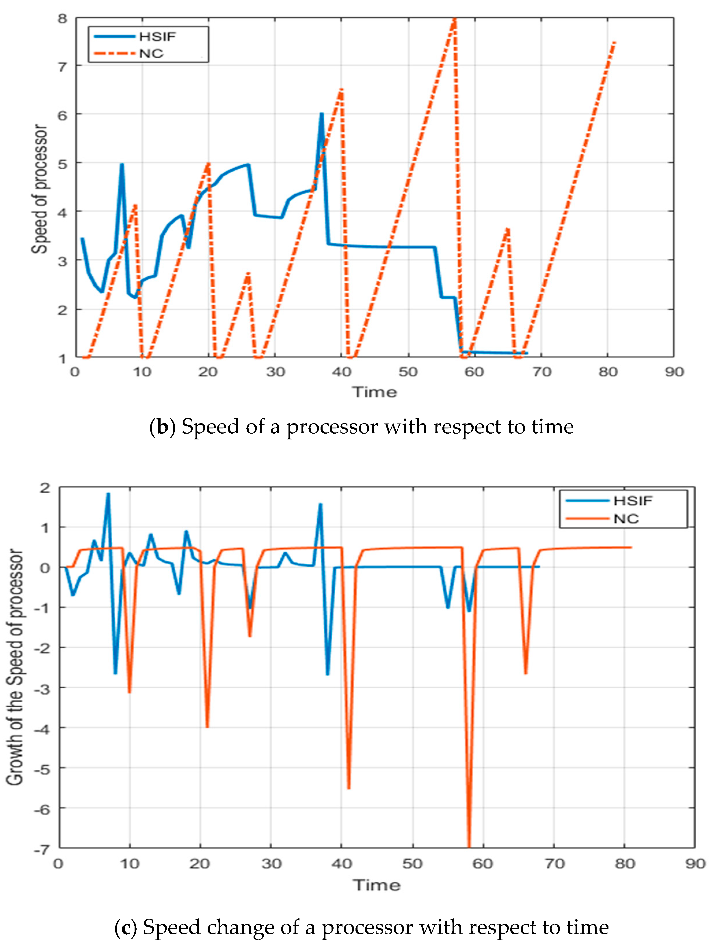
After observing the graphs of Figure 1a,b, it is clear that the HSIF adjusts the sum of the importance of active jobs frequently (count of maxima), but the change in the values is small (difference in the consecutive maxima). This shows that HSIF is maintaining the consistency in the performance. The speed of a processor depends on the sum of importance; therefore, the speed of a processor is having the same reflection. This frequent but less change in the speed makes the HSIF consistent in performance. In NC, the frequency of change in the sum of the importance of active jobs is lesser, but the difference in the change is very high. The speed of a processor using NC depends on the sum of executed size of active jobs; therefore, the speed of a processor variates highly. This high variation makes the NC less consistent in performance.

In Figure 1c, the number of high speed change (local minima) is six when processor is executing jobs by using NC, which is due to the completion and start of execution of the jobs. There is a big change in the speed of processor when the executing job is changed. There is no affect on the new job’s arrival (accumulation of importance based flow) on the execution speed of executing job. In the speed growth graph of processor using HSIF, more than six maxima and minima are available; it shows that the speed of a processor increases on arrival of a new job, i.e., increases on accumulation of scaled importance based flow time. It eliminates the possibility of starvation condition and improves the performance. It shows that HSIF is capable to adjust the speed for maintaining and improving the performance.

Figure 2a shows that initially, at any time the total energy consumed by processor using HSIF is higher than NC, but at the later stage the total energy consumed by processor using NC increases. The total flowtime of all active jobs when executed using NC is more than HSIF; consequently, the energy consumed by processor when using NC is more than HSIF. The energy consumed by most of the individual jobs when they are executed by HSIF is more than NC, as shown is Figure 2b.

The importance based flow time and importance based flow time plus energy values of individual jobs are shown in the Figure 3 and Figure 4 respectively. Most of the individual jobs are having the lesser values of importance based flow time and importance based flow time plus energy when they are executed by using HSIB than NC. HSIF and NC both are competing to reduce the value of the sum of importance based flow time and importance based flow time plus energy, as shown in Figure 3a and Figure 4a, respectively. In the later stage the total values for HSIF is lesser than NC. The total value of importance based flow time and importance based flow time plus energy for a processor by using HSIF is lesser than NC. The value of objective considered is lesser at most of the time when using HSIF. From the above observation, it is concluded that the performance of the HSIF is better and consistent than the best known algorithm NC.

To extend the analysis of the performance of HSIF, a second set of ten jobs and the traditional power model is considered. The jobs arrived along with their importance but the size of jobs was only known at their completion. This case is designed by assuming that the jobs arrive in the increasing order of size. The jobs are executed by using algorithms HSIF and NC (the best known to date [11]); their executions are simulated. The analysed data is mentioned in the

Table 5. Details and execution information of jobs with increasing-order of size using HSIF and NC.

Job	Arrival Time	Importance	Size	Completion Time		Turnaround Time		Response Time
				HSIF	NC	HSIF	NC	HSIF	NC
J1	1	3	5	4	5	3	4	0	0
J2	3	6	6	7	11	4	8	2	3
J3	7	5	8	10	18	3	11	1	5
J4	9	1	10	15	25	6	16	2	10
J5	10	2	10	44	32	34	22	29	16
J6	15	8	14	19	41	4	26	1	18
J7	15	4	17	38	50	23	35	19	27
J8	18	7	21	23	60	5	42	2	33
J9	20	9	22	28	71	8	51	4	41
J10	28	9	23	33	82	5	54	1	44
Average values						9.5	26.9	6.1	19.7

and

Table 6. Three objectives values for jobs arriving with increasing-order of size using HSIF and NC.

Job	Energy Consumed by Individual Job		Importance Based Flow Time of Individual Job		Importance Based Flow Time Plus Energy of Individual Job
	HSIF	NC	HSIF	NC	HSIF	NC
J1	15.5376	11.41421	33.58979	47.65685	49.12738	60.07107
J2	30.39531	18.67619	86.8327	140.9953	117.228	159.6715
J3	20.89599	28.23206	50.98298	291.4622	71.87897	319.6943
J4	7.883328	30.23206	30.62239	466.6225	38.50572	496.8546
J5	134.5865	30.23206	2437.376	648.0149	2571.962	678.2469
J6	40.10598	58.05148	114.9347	1445.479	155.0407	1503.531
J7	169.0947	61.05148	2119.993	2075.943	2289.088	2136.994
J8	48.41263	82.24247	166.9621	3353.273	215.3747	3435.516
J9	95.6372	104.5797	452.1316	5172.41	547.7688	5276.99
J10	52.16065	105.5797	171.5501	5541.149	223.7107	5646.729
Total	614.7099	530.2914	5664.975	19183.01	6279.685	19714.3

. In the Table 5 the job’s arrival time and importance are mentioned. The size is computed and observed at the completion of the jobs. On the basis of the arrival time, starting time of execution and computed completion time the metrics of quality are computed. In this analysis, the metrics of quality considered are turnaround time, response time, power consumed and important based flow time. The computed results are mentioned in the Table 5 and Table 6. The lower values computed using HSIF and NC are marked in bold. The jobs details such as arrival time, completion time importance and size are same for table as well as Table 6.

In Table 5, the turnaround time of nine jobs (out of ten) is lesser using HSIF than NC. It is clearly visible from the data of Table 4 that nine jobs are having response time lesser using HSIF than NC. As well as the average value of turnaround time and response time is lesser using HSIF than NC. On the basis of such observations one can conclude that the working of HSIF is better than the best-known NC in the special case also where the jobs may arrive in the increasing order of size. In Table 6, three values of three objectives energy consumed, importance-based flow time and importance-based flow time plus energy are mentioned. As per the values of energy consumed by the jobs six out of ten jobs consumes lesser power using HSIF than NC; although, the total energy consumed by all ten jobs is more using HSIF than NC. The importance is one of the main factors which forced the schedule of execution of the jobs. The importance based flow times of eight jobs (out of ten) are lesser using HSIF than NC. It is clearly visible from the data of Table 6 that the total importance based flow times of all ten jobs are also lesser using HSIF than NC. This lesser value of metric reflects the better performance of HSIF than NC. The third metric importance-based flow time plus energy (the main objective of the proposed algorithm) of eight jobs (out of ten) are lesser using HSIF than NC. As well as this, the average values of importance-based flow time plus energy of all ten jobs lesser using HSIF than NC. It can be concluded from the observations mentioned above that the objective is better fulfilled by HSIF than NC.

To extend the analysis and increase the performance evaluation, a set of fifty arbitrary jobs with arbitrary arrival time is considered. The size of jobs is computed at the completion time only. Five different objective sets of values turnaround time, completion time, response time, important based flow time, and importance-based flow time plus energy are computed. The simulation results are stated in the

Table 7. Details and execution information of jobs with random-order of size and importance using HSIF and NC.

Job	Arrival Time	Importance	Size	Density	Completion Time		Turnaround Time		Response Time
					HSIF	NC	HSIF	NC	HSIF	NC
J1	1	5	5.6606	1.13212	3	4	2	3	0	0
J2	4	9	11.2292	1.2476889	7	9	3	5	1	1
J3	6	4	6.9192	1.7298	9	15	3	9	2	8
J4	7	5	20.1173	4.02346	17	13	10	6	7	3
J5	10	10	9.6771	0.96771	12	34	2	24	1	22
J6	12	9	4.4418	0.4935333	13	42	1	30	1	26
J7	15	19	29.5157	1.5534579	23	20	8	5	3	1
J8	17	1	10.4579	10.4579	40	22	23	5	19	4
J9	22	2	15.2929	7.64645	33	25	11	3	7	1
J10	23	6	17.6643	2.94405	28	29	5	6	1	3
J11	28	3	5.3368	1.7789333	35	31	7	3	6	2
J12	35	2	9.6688	4.8344	43	37	8	2	6	0
J13	42	7	13.2021	1.8860143	74	63	32	21	31	20
J14	43	13	40.2411	3.0954692	49	49	6	6	1	1
J15	45	14	25.5583	1.8255929	52	66	7	21	5	19
J16	48	8	40.853	5.106625	56	54	8	6	5	2
J17	50	11	12.1269	1.1024455	66	105	16	55	15	54
J18	52	15	54.83	3.6553333	62	59	10	7	7	3
J19	53	16	26.8655	1.6790938	58	76	5	23	4	21
J20	55	7	14.0554	2.0079143	78	61	23	6	22	5
J21	55	9	12.1621	1.3513444	67	99	12	44	11	43
J22	57	17	10.3702	0.6100118	65	127	8	70	7	66
J23	57	19	11.8838	0.6254632	64	122	7	65	6	63
J24	57	20	13.2365	0.661825	63	119	6	62	5	60
J25	57	6	7.5921	1.26535	104	101	47	44	46	43
J26	66	12	11.5422	0.96185	69	110	3	44	2	43
J27	66	7	9.5916	1.3702286	102	91	48	25	47	24
J28	66	11	37.0895	3.3717727	72	73	6	7	4	5
J29	66	14	12.1389	0.8670643	68	114	2	48	1	47
J30	66	8	13.9307	1.7413375	84	74	18	8	17	7
J31	66	8	40.5456	5.0682	87	69	21	3	18	1
J32	66	11	12.1144	1.1013091	73	106	7	40	6	39
J33	70	5	5.3607	1.07214	106	108	36	38	35	38
J34	70	6	6.5298	1.0883	105	107	35	37	34	37
J35	70	7	8.6447	1.2349571	103	103	33	33	32	0
J36	70	8	12.6466	1.580825	93	82	23	12	22	11
J37	73	17	13.2672	0.7804235	75	116	2	43	1	42
J38	74	19	28.4346	1.4965579	77	85	3	11	2	9
J39	74	5	8.0565	1.6113	108	80	34	6	32	7
J40	76	9	13.8968	1.5440889	88	82	12	6	11	7
J41	76	4	2.2268	0.5567	109	131	33	55	32	52
J42	76	8	11.3447	1.4180875	100	85	24	9	23	10
J43	76	11	29.6523	2.6956636	82	78	6	2	4	1
J44	77	15	28.0842	1.87228	80	79	3	2	2	3
J45	81	16	14.7864	0.92415	83	112	2	31	1	30
J46	81	9	12.1814	1.3534889	99	92	18	11	17	10
J47	81	8	10.531	1.316375	101	99	20	18	19	19
J48	87	17	54.2747	3.1926294	92	90	5	3	2	0
J49	93	19	40.1127	2.1111947	98	95	5	2	2	0
J50	93	20	28.3624	1.41812	95	98	2	5	1	3
Total							671	1030	586	916

and

Table 8. Three objectives values for jobs arriving with random-order of size using HSIF and NC.

Job	Energy Consumed by Individual Job (ECiJ)		Importance Based Flow Time of Individual Job (IbFTiJ)		Importance Based Flow Time Plus Energy of Individual Job (ECiJ+IbFTiJ)
	HSIF	NC	HSIF	NC	HSIF	NC
J1	22.3590357	6.770212252	37.835144	21.78250015	59.19418	28.55271241
J2	46.61278883	36.02011586	100.76936	149.8960335	147.3821	185.9161493
J3	19.25226637	40.5746285	49.274854	228.881385	68.52712	269.4560135
J4	82.78841236	64.15138995	516.081	323.9872543	598.8694	388.1386443
J5	32.71807139	229.7936205	65.670287	2770.892657	98.38836	3000.686277
J6	20.23553431	237.102096	31.471069	3251.6285	51.7066	3488.730596
J7	202.7829624	100.2795249	983.04991	428.7590059	1185.833	529.0385308
J8	42.27367303	60.70577844	529.99832	345.0057207	572.272	405.7114991
J9	33.7634238	150.0710023	215.89783	545.5858599	249.6613	695.6568622
J10	42.07948789	114.1502519	134.28054	647.9364288	176.36	762.0866808
J11	34.33977776	14.82308387	158.99266	43.4028688	193.3324	58.22595267
J12	25.33865247	59.42091636	102.66566	97.67231059	128.0043	157.093227
J13	481.3604361	161.075095	8793.2476	1932.709082	9274.608	2093.784177
J14	85.00788703	276.5769064	315.44764	1565.904674	400.4555	1842.48158
J15	152.3533413	341.901121	692.16774	4081.84265	844.5211	4423.743771
J16	168.7093341	444.4016939	839.37168	2652.137703	1008.081	3096.539397
J17	336.5378155	607.6676007	3232.0993	17099.83442	3568.637	17707.50202
J18	235.6998431	431.6038271	1408.9237	2838.699032	1644.624	3270.302859
J19	127.5172457	376.2169431	458.29066	4628.367088	585.8079	5004.584031
J20	326.6801405	58.09137545	4373.3849	265.635671	4700.065	323.7270464
J21	197.7173871	396.6756722	1471.3821	8940.40525	1669.1	9337.080922
J22	236.5408466	1136.468047	1249.902	38599.64292	1486.443	39736.11097
J23	228.3316502	1206.144663	1083.7848	38904.03481	1312.116	40110.17947
J24	203.5856335	1213.137134	857.18131	37422.77458	1060.767	38635.91172
J25	645.8262181	264.632675	17000.018	5968.470375	17645.84	6233.10305
J26	61.42174437	526.4527132	160.7368	11821.89117	222.1585	12348.34388
J27	551.6457635	175.6851143	11254.291	2292.812971	11805.94	2468.498086
J28	100.7695008	196.6953921	406.78459	1250.246015	507.5541	1446.941407
J29	50.85532029	666.0633792	106.35154	16186.67205	157.2069	16852.73543
J30	280.5938868	64.87066875	2998.2111	295.8360188	3278.805	360.7066875
J31	318.7016553	216.3189596	3782.0731	771.3952677	4100.775	987.7142273
J32	132.192008	442.7510756	627.45436	9143.243446	759.6464	9585.994522
J33	394.0326882	190.53607	8038.7794	3725.90673	8432.812	3916.4428
J34	457.5086268	222.54415	9087.2176	4238.6777	9544.726	4461.22185
J35	498.2490083	231.6174786	9359.2487	3947.994271	9857.498	4179.61175
J36	373.348732	96.7904125	4998.1542	634.2753625	5371.503	731.065775
J37	61.75288892	720.4549719	129.14116	15634.62855	190.894	16355.08352
J38	91.44826525	212.2669018	234.05556	1311.454543	325.5038	1523.721444
J39	362.0526921	35.80565	6900.7966	146.4452	7262.849	182.25085
J40	197.7173871	63.77204444	1471.3821	258.1763556	1669.1	321.9484
J41	284.713719	210.1924482	5348.1421	5632.759218	5632.856	5842.951667
J42	392.3744651	80.70904375	5464.8046	447.7994813	5857.179	528.508525
J43	106.386545	53.26049632	437.28887	136.4336571	543.6754	189.6941535
J44	72.19599888	58.38507639	184.7807	157.6041655	256.9767	215.9892419
J45	58.12036605	489.3002581	121.54462	7737.146183	179.665	8226.446441
J46	315.6681227	99.67674444	3372.9875	602.1209333	3688.656	701.7976778
J47	317.1910961	152.6581875	3732.1705	1533.16375	4049.362	1685.821938
J48	117.5735219	291.1073658	405.47938	974.5465744	523.0529	1265.65394
J49	142.6166731	93.38620681	503.28556	247.963412	645.9022	341.3496188
J50	65.43614279	119.1602493	131.34057	454.3746597	196.7767	573.534909
Total	9834.978683	13738.91643	123957.6903	263339.4565	133791.6699	277078.3729

.

On the simulation data provided in the Table 7 and Table 8, the statistical analysis is conducted. The Independent Samples t Test is used to compare the means of two independent groups in order to determine whether there is statistical evidence that the associated objective means are significantly different.

In the first

Table 9. Group statistics of objectives values for HSIF and NC.

Group Statistics
	Scheduling	N	Mean (M)	Std. Deviation (s)	Std. Error Mean
Turnaround_time	HSIF	50	13.42	12.511366	1.7693744
	NC	50	20.6	19.786617	2.7982502
Responce_time	HSIF	50	11.72	12.748813	1.8029545
	NC	50	18.32	19.976966	2.8251697
Completion_time	HSIF	50	67.4	30.651431	4.3347669
	NC	50	74.82	34.902014	4.9358902
Energy_consumed	HSIF	50	196.7	160.31869	22.672486
	NC	50	274.778	291.01057	41.155109
Importance_based_flow_time	HSIF	50	2479.15	3625.2051	512.68143
	NC	50	15373.3	21122.893	2987.2282
Importance_based_flow_time_plus_energy	HSIF	50	2675.83	3774.8105	533.83883
	NC	50	5541.57	9740.346	1377.4929

, Group Statistics, provides basic information about the group comparisons, including the sample size (n), mean, standard deviation, and standard error for objectives by group. In the second section, Independent Samples Test, displays the results most relevant to the Independent Samples t Test. There are two parts that provide different pieces of information: t-test for Equality of Means and Levene’s Test for Equality of Variances. If the p value is less than or equal to the 0.05, then one should use the lower row of the output (the row labeled “Equal variances not assumed”). If the p value is greater than 0.05, then one should use the upper row of the output (the row labeled “Equal variances assumed”). Based on the results provided in the Table 9 and

Table 10. Statistics of objectives values for HSIF and NC using Independent Samples t Test.

Independent Samples Test
Objectives		t-Test for Equality of Means							Levene’s Test for Equality of Variances
		t	df	p-Value (2-tailed)	Mean Difference	Std. Error Difference	95% Confidence Interval of the Difference		F	p-Value
							Lower	Upper
Turnaround_Time	Equal Variances Assumed	−2.17	98	0.033	−7.18	3.31072346	−13.7500229	−0.60997705	14.19	0
	Equal Variances Not assumed	−2.17	82.78	0.033	−7.18	3.31072346	−13.765152	−0.59484797
Responce_Time	Equal Variances Assumed	−1.97	98	0.05	−6.6	3.35145171	−13.2508468	0.050846846	13.27	0
	Equal Variances Not assumed	−1.97	83.23	0.05	−6.6	3.35145171	−13.2656255	0.065625546
Completion_Time	Equal Variances Assumed	−1.13	98	0.261	−7.42	6.56911077	−20.4561865	5.616186531	1.277	0.26
	Equal variances Not assumed	−1.13	96.39	0.261	−7.42	6.56911077	−20.4589043	5.618904335
Energy_Consumed	Equal Variances Assumed	−1.66	98	0.1	−78.078755	46.9870691	−171.323064	15.16555442	5.645	0.02
	Equal Variances Not assumed	−1.66	76.23	0.101	−78.078755	46.9870691	−171.656969	15.499459
Importance_based_flow_time	Equal Variances Assumed	−1.95	98	0.05	−2787.635324	1432.92269	−5631.22377	55.95311792	9.168	0
	Equal Variances Not assumed	−1.95	63.08	0.05	−2787.635324	1432.92269	−5651.02882	75.75817343
Importance_Based_Flow_time_plus_energy	Equal Variances Assumed	−1.94	98	0.05	−2865.734061	1477.31876	−5797.42506	65.95693429	8.953	0
	Equal Variances Not assumed	−1.94	63.39	0.05	−2865.734061	1477.31876	−5817.56103	86.09291177

, the following conclusive remarks are considered:

• For Turnaround Time p-value is less than 0.05 in Levene’s Test for Equality of Variances; therefore, the null hypothesis (the variability of the two groups is equal) is rejected. The lower row of the output (the row labeled “Equal variances not assumed”) is considered. A t test passed to reveal a statistically reliable difference between the mean values of Turnaround Time of HSIF (M = 13.42, s = 12.511366261) and NC (M = 20.6, s = 19.786616792) with t(82.782) = 2.17, p = 0.033.
• The total Turnaround Time for HSIF is 359 time unit lesser than the total Turnaround Time for NC. The average Turnaround Time for HSIF is 7.18 time unit lesser than the average Turnaround Time for NC.
• For Response Time p-value is less than 0.05 in Levene’s Test for Equality of Variances; therefore, the null hypothesis (the variability of the two groups is equal) is rejected. The lower row of the output (the row labeled “Equal variances not assumed”) is considered. A t test passed to reveal a statistically reliable difference between the mean values of Response Time of HSIF (M = 11.72, s = 12.748813) and NC (M = 18.32, s = 19.976966) with t(83.23) = 2.17, p = 0.05.
• The total Response Time for HSIF is 330 time unit lesser than the total Response Time for NC. The average Response Time for HSIF is 6.6 time unit lesser than the average Response Time for NC.
• For Completion Time p-value is greater than 0.05 in Levene’s Test for Equality of Variances; therefore, the null hypothesis (the variability of the two groups is equal) is considered. The upper row of the output (the row labeled “Equal variances assumed”) is considered. A t test failed to reveal a statistically reliable difference between the mean values of Completion Time of HSIF (M = 67.4, s = 30.651431) and NC (M = 74.82, s = 34.902014) with t(98) = 1.13, p = 0.261.
• For Energy Consumed p-value is greater than 0.05 in Levene’s Test for Equality of Variances; therefore, the null hypothesis (the variability of the two groups is equal) is considered. The upper row of the output (the row labeled “Equal variances assumed”) is considered. A t test failed to reveal a statistically reliable difference between the mean values of Energy Consumed of HSIF (M = 196.7, s = 160.31869) and NC (M = 274.778, s = 291.01057) with t(98) = 1.66, p = 0. 1.
• Although, the statistical test failed to identify the difference in HSIF and NC on the basis of energy consumed, the total Energy Consumed for HSIF is 3909.937747 unit lesser than the total Energy Consumed for NC. The average Energy Consumed for HSIF is 78.07875 unit lesser than the average Energy Consumed for NC.
• For Importance-based Flow Time p-value is less than 0.05 in Levene’s Test for Equality of Variances; therefore, the null hypothesis (the variability of the two groups is equal) is rejected. The lower row of the output (the row labeled “Equal variances not assumed”) is considered. A t test passed to reveal a statistically reliable difference between the mean values of Importance-based Flow Time of HSIF (M = 2479.15, s = 3625.2051) and NC (M = 15373.3, s = 21122.893) with t(63.08) = 1.95, p = 0.05.
• The total Importance-based Flow Time for HSIF is 139381.7662 unit lesser than the total Importance-based Flow Time for NC. The average Importance-based Flow Time for HSIF is 2787.635324 unit lesser than the average Importance-based Flow Time for NC.
• For Importance-based Flow Time plus Energy p-value is less than 0.05 in Levene’s Test for Equality of Variances; therefore, the null hypothesis (the variability of the two groups is equal) is rejected. The lower row of the output (the row labeled “Equal variances not assumed”) is considered. A t test passed to reveal a statistically reliable difference between the mean values of Importance-based Flow Time plus Energy of HSIF (M = 2675.83, s = 3774.8105) and NC (M = 5541.57, s = 9740.346) with t(63.39) = 1.94, p = 0.05.
• The total Importance-based Flow Time plus Energy for HSIF is 143286.703 unit lesser than the total Importance-based Flow Time plus Energy for NC. The average Importance-based Flow Time plus Energy for HSIF is 2865.73406 unit lesser than the average Importance-based Flow Time plus Energy for NC.

It is clearly evident from the above statistical analysis and deduced results that HSIF performance better than the best available scheduling algorithm NC.

To extend the perfection of the analysis of the evaluation of working of HSIF in comparison to NC, the normalized Z-values of Energy Consumed by individual job (ECiJ) and importance-based flow time of individual job (IbFTiJ) are computed and provided in the

Table 11. Normalized objectives values for HSIF using z-score.

Job	Simple Values		Z Values		Sum (ZHSIF_ECiJ + ZHSIF_IbFTiJ)	Normalized Sum (in range [0 1])
	HSIF_ECiJ	HSIF_IbFTiJ	ZHSIF_ECiJ	ZHSIF_IbFTiJ
J1	22.359	37.835144	−1.08746	−0.67343	−1.76089	0.147822
J2	46.6128	100.76936	−0.93618	−0.65607	−1.59225	0.18155
J3	19.2523	49.274854	−1.10684	−0.67027	−1.77711	0.144578
J4	82.7884	516.081	−0.71053	−0.54151	−1.25204	0.249592
J5	32.7181	65.670287	−1.02285	−0.66575	−1.6886	0.16228
J6	20.2355	31.471069	−1.10071	−0.67518	−1.77589	0.144822
J7	202.783	983.04991	0.03795	−0.41269	−0.37474	0.425052
J8	42.2737	529.99832	−0.96324	−0.53767	−1.50091	0.199818
J9	33.7634	215.89783	−1.01633	−0.62431	−1.64064	0.171872
J10	42.0795	134.28054	−0.96445	−0.64682	−1.61127	0.177746
J11	34.3398	158.99266	−1.01273	−0.64001	−1.65274	0.169452
J12	25.3387	102.66566	−1.06888	−0.65555	−1.72443	0.155114
J13	481.3604	8793.2476	1.77559	1.74172	3.51731	1.203462
J14	85.0079	315.44764	−0.69669	−0.59685	−1.29354	0.241292
J15	152.3533	692.16774	−0.27661	−0.49293	−0.76954	0.346092
J16	168.7093	839.37168	−0.17459	−0.45233	−0.62692	0.374616
J17	336.5378	3232.0993	0.87225	0.2077	1.07995	0.71599
J18	235.6998	1408.9237	0.24327	−0.29522	−0.05195	0.48961
J19	127.5172	458.29066	−0.43153	−0.55745	−0.98898	0.302204
J20	326.6801	4373.3849	0.81076	0.52252	1.33328	0.766656
J21	197.7174	1471.3821	0.00635	−0.27799	−0.27164	0.445672
J22	236.5408	1249.902	0.24851	−0.33908	−0.09057	0.481886
J23	228.3317	1083.7848	0.19731	−0.38491	−0.1876	0.46248
J24	203.5856	857.18131	0.04295	−0.44742	−0.40447	0.419106
J25	645.8262	17000.018	2.80146	4.00553	6.80699	1.861398
J26	61.4217	160.7368	−0.84381	−0.63953	−1.48334	0.203332
J27	551.6458	11254.291	2.214	2.42059	4.63459	1.426918
J28	100.7695	406.78459	−0.59837	−0.57166	−1.17003	0.265994
J29	50.8553	106.35154	−0.90971	−0.65453	−1.56424	0.187152
J30	280.5939	2998.2111	0.5233	0.14318	0.66648	0.633296
J31	318.7017	3782.0731	0.761	0.35941	1.12041	0.724082
J32	132.192	627.45436	−0.40237	−0.51078	−0.91315	0.31737
J33	394.0327	8038.7794	1.23088	1.5336	2.76448	1.052896
J34	457.5086	9087.2176	1.62682	1.82281	3.44963	1.189926
J35	498.249	9359.2487	1.88094	1.89785	3.77879	1.255758
J36	373.3487	4998.1542	1.10186	0.69486	1.79672	0.859344
J37	61.7529	129.14116	−0.84174	−0.64824	−1.48998	0.202004
J38	91.4483	234.05556	−0.65651	−0.6193	−1.27581	0.244838
J39	362.0527	6900.7966	1.0314	1.21969	2.25109	0.950218
J40	197.7174	1471.3821	0.00635	−0.27799	−0.27164	0.445672
J41	284.7137	5348.1421	0.54899	0.7914	1.34039	0.768078
J42	392.3745	5464.8046	1.22054	0.82358	2.04412	0.908824
J43	106.3865	437.28887	−0.56333	−0.56324	−1.12657	0.274686
J44	72.196	184.7807	−0.7766	−0.63289	−1.40949	0.218102
J45	58.1204	121.54462	−0.8644	−0.65034	−1.51474	0.197052
J46	315.6681	3372.9875	0.74208	0.24656	0.98864	0.697728
J47	317.1911	3732.1705	0.75158	0.34564	1.09722	0.719444
J48	117.5735	405.47938	−0.49355	−0.57202	−1.06557	0.286886
J49	142.6167	503.28556	−0.33735	−0.54504	−0.88239	0.323522
J50	65.4361	131.34057	−0.81877	−0.64764	−1.46641	0.206718
Average	196.69957	2479.153805	2 × 10−7	8.88178 × 10−18	2 × 10−7	0.50000004
Total	9834.9785	123957.6903	1 × 10−5	0	1 × 10−5	25.000002

and

Table 12. Normalized objectives values for NC using z-score.

Job	Simple Values		Z Values		Sum (ZNC_ECiJ + ZNC_IbFTiJ)	Normalized Sum (in range [0 1])
	NC_ECiJ	NC_IbFTiJ	ZNC_ECiJ	ZNC_IbFTiJ
J1	6.7702	21.7825	−0.92096	−0.55435	−1.47531	0.204938
J2	36.0201	149.896034	−0.82045	−0.54081	−1.36126	0.227748
J3	40.5746	228.881385	−0.80479	−0.53246	−1.33725	0.23255
J4	64.1514	323.987254	−0.72378	−0.52241	−1.24619	0.250762
J5	229.7936	2770.892657	−0.15458	−0.26379	−0.41837	0.416326
J6	237.1021	3251.6285	−0.12947	−0.21298	−0.34245	0.43151
J7	100.2795	428.759006	−0.59963	−0.51133	−1.11096	0.277808
J8	60.7058	345.005721	−0.73562	−0.52019	−1.25581	0.248838
J9	150.071	545.58586	−0.42853	−0.49899	−0.92752	0.314496
J10	114.1503	647.936429	−0.55197	−0.48817	−1.04014	0.291972
J11	14.8231	43.402869	−0.89328	−0.55206	−1.44534	0.210932
J12	59.4209	97.672311	−0.74003	−0.54633	−1.28636	0.242728
J13	161.0751	1932.709082	−0.39072	−0.35238	−0.7431	0.35138
J14	276.5769	1565.904674	0.00618	−0.39115	−0.38497	0.423006
J15	341.9011	4081.84265	0.23065	−0.12524	0.10541	0.521082
J16	444.4017	2652.137703	0.58288	−0.27634	0.30654	0.561308
J17	607.6676	17099.83442	1.14391	1.25064	2.39455	0.97891
J18	431.6038	2838.699032	0.5389	−0.25663	0.28227	0.556454
J19	376.2169	4628.367088	0.34857	−0.06748	0.28109	0.556218
J20	58.0914	265.635671	−0.7446	−0.52858	−1.27318	0.245364
J21	396.6757	8940.40525	0.41888	0.38827	0.80715	0.66143
J22	1136.468	38599.64292	2.96103	3.52297	6.484	1.7968
J23	1206.1447	38904.03481	3.20046	3.55515	6.75561	1.851122
J24	1213.1371	37422.77458	3.22448	3.39859	6.62307	1.824614
J25	264.6327	5968.470375	−0.03486	0.07416	0.0393	0.50786
J26	526.4527	11821.89117	0.86483	0.69281	1.55764	0.811528
J27	175.6851	2292.812971	−0.34051	−0.31432	−0.65483	0.369034
J28	196.6954	1250.246015	−0.26832	−0.42451	−0.69283	0.361434
J29	666.0634	16186.67205	1.34457	1.15413	2.4987	0.99974
J30	64.8707	295.836019	−0.72131	−0.52538	−1.24669	0.250662
J31	216.319	771.395268	−0.20088	−0.47512	−0.676	0.3648
J32	442.7511	9143.243446	0.5772	0.40971	0.98691	0.697382
J33	190.5361	3725.90673	−0.28948	−0.16286	−0.45234	0.409532
J34	222.5442	4238.6777	−0.17949	−0.10866	−0.28815	0.44237
J35	231.6175	3947.994271	−0.14831	−0.13938	−0.28769	0.442462
J36	96.7904	634.275363	−0.61162	−0.48961	−1.10123	0.279754
J37	720.455	15634.62855	1.53148	1.09578	2.62726	1.025452
J38	212.2669	1311.454543	−0.21481	−0.41804	−0.63285	0.37343
J39	35.8057	146.4452	−0.82118	−0.54117	−1.36235	0.22753
J40	63.772	258.176356	−0.72508	−0.52936	−1.25444	0.249112
J41	210.1924	5632.759218	−0.22194	0.03868	−0.18326	0.463348
J42	80.709	447.799481	−0.66688	−0.50932	−1.1762	0.26476
J43	53.2605	136.433657	−0.7612	−0.54223	−1.30343	0.239314
J44	58.3851	157.604166	−0.74359	−0.53999	−1.28358	0.243284
J45	489.3003	7737.146183	0.73716	0.26109	0.99825	0.69965
J46	99.6767	602.120933	−0.6017	−0.49301	−1.09471	0.281058
J47	152.6582	1533.16375	−0.41964	−0.39461	−0.81425	0.33715
J48	291.1074	974.546574	0.05611	−0.45365	−0.39754	0.420492
J49	93.3862	247.963412	−0.62332	−0.53044	−1.15376	0.269248
J50	119.1602	454.37466	−0.53475	−0.50863	−1.04338	0.291324
Average	274.77833	5266.789129	2 × 10−7	4 × 10−7	6 × 10−7	0.50000012
Total	13738.9165	263339.4565	1 × 10−5	2 × 10−5	3 × 10−5	25.000006

. The sum of Z values of Energy Consumed by individual job (ECiJ) and the importance-based flow time of individual job (IbFTiJ) are added and converted in to the range [0 1] for individual job, as shown in the Table 11 and Table 12. For all jobs, the total of normalized values of ECiJ+IbFTiJ and the average of the normalized values of ECiJ+IbFTiJ are provided (in the Table 11 and Table 12) to reflect the difference between the working of both algorithms. The normalized total values and average values of ECiJ+IbFTiJ are lesser for HSIF than NC. It reflects that the normalized value of dual objective (i.e., the sum of energy consumed and importance based flow time) for HSIF is lesser and better than NC. It is concluded from the above analysis that HSIF performs better than NC.

6. Conclusions and Future Work

An online non-clairvoyant job scheduling algorithm Highest Scaled Importance First (HSIF) is proposed with an objective to minimize the sum of scaled importance based flow time and energy consumed. HSIF uses the arbitrary power function and dynamic speed scaling policy for uni-processor system. The working of HSIF is analysed using the amortized potential function analysis against an optimal offline adversary. The competitive ratio of HSIF is 2. The competitive ratio of HSIF is lesser than the non-clairvoyant scheduling algorithms LAPS, SelMig, NC, ${\mathrm{R}}^3$, EtRR, ALG, and WLAPS; similar to an online clairvoyant scheduling Alg. Additionally, a set of jobs is considered as an illustrative example and the execution of the jobs on a processor is simulated by using HSIF and the best known algorithm NC. The simulation results show that the performance of the HSIF is consistent and better than the other online non-clairvoyant algorithm. On the basis of amortized potential function analysis and simulation results, it is concluded that the HSIF performs better than any other online non-clairvoyant algorithm. Use of HSIF in data centres and in battery based devices will reduce power consumption and improve computing capability. The further enhancement of our study will be to evaluate the working of HSIF in the multi-processor environment and the experiments will be conducted in the real time environment as well as with more number of test cases. Along with the amortized analysis and simulation the result will be analysed using statistical tests. The working of HSIF will be evaluated in the cloud/fog environment for resource allocation and energy optimization. One open problem is to reduce the competitive ratio that is achieved in this paper. In the further extension of this work, the number of jobs may be increased significantly to enhance the analysis of the algorithmic evaluation.

References

- Singh, P. Prashast Release Round Robin: R3 an energy-aware non-clairvoyant scheduling on speed bounded processors. Karbala Int. J. Mod. Sci. 2015, 1, 225–236. [Google Scholar] [CrossRef]
- Singh, P.; Wolde-Gabriel, B. Executed-time Round Robin: EtRR an online non-clairvoyant scheduling on speed bounded processor with energy management. J. King Saud Univ. Comput. Inf. Sci. 2016, 29, 74–84. [Google Scholar] [CrossRef]
- U.S. Environmental Protection Agency. EPA Report on server and data centre energy efficiency. Available online: https://www.energystar.gov/index.cfm?c=prod_development.server_efficiency_study (accessed on 10 June 2015).
- Shehabi, A.; Smith, S.J.; Masanet, E.; Koomey, J. Data center growth in the United States: Decoupling the demand for services from electricity use. Environ. Res. Lett. 2018, 13, 1–12. [Google Scholar] [CrossRef]
- Fernández-Cerero, D.; Jakobik, A.; Grzonka, D.; Kołodziej, J.; Fernandez-Montes, A. Security supportive energy-aware scheduling and energy policies for cloud environments. J. Parallel Distrib. Comput. 2018, 119, 191–202. [Google Scholar] [CrossRef]
- Lei, H.; Wang, R.; Zhang, T.; Liu, Y.; Zha, Y. A multi-objective co-evolutionary algorithm for energy-efficient scheduling on a green data center. Comput. Oper. Res. 2016, 75, 103–117. [Google Scholar] [CrossRef]
- Chan, H.-L.; Edmonds, J.; Pruhs, K. Speed Scaling of Processes with Arbitrary Speedup Curves on a Multiprocessor. Theory Comput. Syst. 2011, 49, 817–833. [Google Scholar] [CrossRef] [Green Version]
- Bansal, N.; Kimbrel, T.; Pruhs, K. Dynamic speed scaling to manage energy and temperature. J. ACM 2007, 54, 1–39. [Google Scholar] [CrossRef]
- Pruhs, K.; Uthaisombut, P.; Woeginger, G. Getting the best response for your erg. ACM Trans. Algorithms 2008, 4, 1–17. [Google Scholar] [CrossRef] [Green Version]
- Bansal, N.; Chan, H.L.; Pruhs, K. Speed scaling with an arbitrary power function. In Proceedings of the Annual ACM-SIAM Symposium on Discrete Algorithms, New York, NY, USA, 4–6 January 2009; pp. 693–701. [Google Scholar]
- Azar, Y.; Devanur, N.R.; Huang, Z.; Panigrahi, D. Speed Scaling in the Non-clairvoyant Model. In Proceedings of the Annual ACM Symposium on Parallelism in Algorithms and Architectures, Portland, OR, USA, 13–15 June 2015; pp. 133–142. [Google Scholar]
- Bansal, N.; Pruhs, K.; Stein, C. Speed Scaling for Weighted Flow Time. SIAM J. Comput. 2009, 39, 1294–1308. [Google Scholar] [CrossRef]
- Motwani, R.; Phillips, S.; Torng, E. Nonclairvoyant scheduling. Theor. Comput. Sci. 1994, 30, 17–47. [Google Scholar] [CrossRef]
- Bansal, N.; Dhamdhere, K.; Konemann, J.; Sinha, A. Non-clairvoyant Scheduling for Minimizing Mean Slowdown. Algorithmica 2004, 40, 305–318. [Google Scholar] [CrossRef]
- Yao, F.; Demers, A.; Shenker, S. A scheduling model for reduced CPU energy. In Proceedings of the Annual Symposium on Foundations of Computer Science, Berkeley, CA, USA, 23–25 October 1995; pp. 374–382. [Google Scholar]
- Leonardi, S.; Raz, D. Approximating total flow time on parallel machines. In Proceedings of the ACM Symposium on Theory of Computing, El Paso, TX, USA, 4–6 May 1997; pp. 110–119. [Google Scholar]
- Chekuri, C.; Khanna, S.; Zhu, A. Algorithms for minimizing weighted flow time. In Proceedings of the ACM Symposium on Theory of Computing, Crete, Greece, 6–8 July 2001; pp. 84–93. [Google Scholar]
- Awerbuch, B.; Azar, Y.; Leonardi, S.; Regev, O. Minimizing the Flow Time Without Migration. SIAM J. Comput. 2002, 31, 1370–1382. [Google Scholar] [CrossRef] [Green Version]
- Avrahami, N.; Azar, Y. Minimizing total flow time and total completion time with immediate dispatching. In Proceedings of the ACM Symposium on Parallelism in Algorithms and Architectures, San Diego, CA, USA, 7–9 June 2003; p. 11. [Google Scholar]
- Chekuri, C.; Goel, A.; Khanna, S.; Kumar, A. Multiprocessor scheduling to minimize flow time with epsilon resource augmentation. In Proceedings of the ACM Symposium on Theory of Computing, Chicago, IL, USA, 13–15 June 2004; pp. 363–372. [Google Scholar]
- Pruhs, K.; Sgall, J.; Torng, E. Online Scheduling. In Handbook of Scheduling: Algorithms, Models, and Performance Analysis, 1st ed.; Leung, J.Y.-T., Ed.; CRC Press: Boca Raton, FL, USA, 2004; pp. 15–41. [Google Scholar]
- Becchetti, L.; Leonardi, S.; Marchetti-Spaccamela, A.; Pruhs, K. Online weighted flow time and deadline scheduling. J. Discret. Algorithms 2006, 4, 339–352. [Google Scholar] [CrossRef] [Green Version]
- Chadha, J.; Garg, N.; Kumar, A.; Muralidhara, V. A competitive algorithm for minimizing weighted flow time on unrelated processors with speed augmentation. In Proceedings of the Annual ACM Symposium on Theory of Computing, Bethesda, MD, USA, 31 May–2 June 2009; pp. 679–684. [Google Scholar]
- Anand, S.; Garg, N.; Kumar, A. Resource Augmentation for Weighted Flow-time explained by Dual Fitting. In Proceedings of the Twenty-Third Annual ACM-SIAM Symposium on Discrete Algorithms, Kyoto, Japan, 17–19 January 2012; pp. 1228–1241. [Google Scholar]
- Albers, S.; Fujiwara, H. Energy-efficient algorithms for flow time minimization. ACM Trans. Algorithms 2007, 3, 49. [Google Scholar] [CrossRef] [Green Version]
- Chan, S.-H.; Lam, T.-W.; Lee, L.-K. Non-clairvoyant Speed Scaling for Weighted Flow Time. In Proceedings of the Annual European Symposium, Liverpool, UK, 6–8 September 2010; pp. 23–35. [Google Scholar]
- Im, S.; Kulkarni, J.; Munagala, K.; Pruhs, K. SelfishMigrate: A Scalable Algorithm for Non-clairvoyantly Scheduling Heterogeneous Processors. In Proceedings of the 2014 IEEE 55th Annual Symposium on Foundations of Computer Science (FOCS), Philadelphia, PA, USA, 18–21 October 2014; pp. 531–540. [Google Scholar]
- Fernández-Cerero, D.; Fernández-Montes, A.; Ortega, J.A. Energy policies for data-center monolithic schedulers. Expert Syst. Appl. 2018, 110, 170–181. [Google Scholar] [CrossRef]
- Duy, T.V.T.; Sato, Y.; Inoguchi, Y. Performance evaluation of a Green Scheduling Algorithm for energy savings in Cloud computing. In Proceedings of the IEEE international Symposium on Parallel & Distributed Processing, Workshops and Phd Forum (IPDPSW), Atlanta, GA, USA, 19–23 April 2010; pp. 1–8. [Google Scholar]
- Beloglazov, A.; Abawajy, J.; Buyya, R. Energy-aware resource allocation heuristics for efficient management of data centers for Cloud computing. Futur. Gener. Comput. Syst. 2012, 28, 755–768. [Google Scholar] [CrossRef] [Green Version]
- Sohrabi, S.; Tang, A.; Moser, I.; Aleti, A. Adaptive virtual machine migration mechanism for energy efficiency. In Proceedings of the 2016 IEEE/ACM 5th International Workshop on Green and Sustainable Software (GREENS), Austin, TX, USA, 16 May 2016; pp. 8–14. [Google Scholar]
- Juarez, F.; Ejarque, J.; Badia, R.M. Dynamic energy-aware scheduling for parallel task-based application in cloud computing. Futur. Gener. Comput. Syst. 2018, 78, 257–271. [Google Scholar] [CrossRef] [Green Version]
- Gupta, A.; Krishnaswamy, R.; Pruhs, K. Scalably Scheduling Power-Heterogeneous Processors. In Proceedings of the 37th International Colloquium Conference on Automata, Languages and Programming, Bordeaux, France, 6–10 July 2010; pp. 312–323. [Google Scholar]
- Sun, H.; He, Y.; Hsu, W.-J.; Fan, R. Energy-efficient multiprocessor scheduling for flow time and makespan. Theor. Comput. Sci. 2014, 550, 1–20. [Google Scholar] [CrossRef] [Green Version]
Figure 1.
The execution results of jobs and processor speed with respect to time.
Figure 2.
Energy Consumption of processes and jobs.
Figure 3.
Importance based flow time of jobs.
Figure 4.
Importance based flow time with energy of jobs.