Numerical Simulation of Multi-Span Greenhouse Structures
by
 , ,
, ,
María S. Fernández-García
1, 
Pablo Vidal-López
1,*,
Desirée Rodríguez-Robles
1,
José R. Villar-García
2 and
Rafael Agujetas
3 1
Department of Forest and Agricultural Engineering, School of Agricultural Engineering, University of Extremadura, Av. Adolfo Suarez s/n, 06071 Badajoz, Spain
2
Department of Forest and Agricultural Engineering, Universitary Center of Plasencia, University of Extremadura, Av. Virgen del Puerto 2, 10600 Plasencia, Spain
3
Department of Mechanical, Energy and Materials Engineering, School of Industrial Engineering, University of Extremadura, Avda. de Elvas s/n, 06006 Badajoz, Spain
*
Author to whom correspondence should be addressed.
Agriculture 2020, 10(11), 499; https://doi.org/10.3390/agriculture10110499
Submission received: 2 October 2020
/
Revised: 21 October 2020
/
Accepted: 22 October 2020
/
Published: 25 October 2020
(This article belongs to the Section Agricultural Technology)
Abstract
:Greenhouses had to be designed to sustain permanent maintenance and crop loads as well as the site-specific climatic conditions, with wind being the most damaging. However, both the structure and foundation are regularly empirically calculated, which could lead to structural inadequacies or cost ineffectiveness. Thus, in this paper, the structural assessment of a multi-tunnel greenhouse was carried out. Firstly, wind loads were assessed through computational fluid dynamics (CFD). Then, the buckling failure mode when either the European Standard (EN) or the CFD wind loads were contemplated was assessed by a finite element method (FEM). Conversely to the EN 13031-1, CFD wind loads generated a suction in the 0–55° region of the first tunnel and a 60% reduction of the external pressure coefficients in the third tunnel was not detected. Moreover, the first-order buckling eigenvalues were reduced (32–57%), which resulted in the need for a different calculation method (i.e., elastoplastic analysis), and global buckling modes similar to local buckling shape were detected. Finally, the foundation was studied by the FEM and a matrix method based on the Wrinkler model. The stresses and deformations arising from the proposed matrix method were conservative compared to those obtained by the FEM.
1. Introduction
Although greenhouses extend all over Europe (Figure 1), the number of these structures are especially predominant in some regions due to the favorable local meteorological circumstances (e.g., Mediterranean climate characterized by warm and humid winters, hot and dry summers and clear days with fairly high radiation even during fall and winter) in which crop production in greenhouses is a rising agricultural sector.
Among European nations (Figure 1), Spain is the country with the highest greenhouse area and accounts for the 35% of the total reported statistics on protected cultivation for the latest available dataset (i.e., 2016) provided by Eurostat [1]. Nonetheless, Italy, France, the Netherlands, Poland and Greece also display greenhouse area values greater than the European average (4729 ha).
Due to the relative importance in Europe, Figure 2 illustrates the evolution of the crop production area under greenhouse in Spain between 2002 and 2019. Although not homogenously, protected horticulture increased up to 28.6% in the last 18 years.
Last available estimates show that 70,744 ha of Spanish crop production occurred in greenhouses [2]. Nonetheless, a great disparity in figures exists among the different Autonomous Communities (Figure 3a). Thus, it is worth mentioning the relevance of Andalusia with 53,902 ha, which represents 76.2% of the country total. Moreover, the Almeria province is the largest contributor with 32,958 ha, i.e., 61.1% of the total Andalusian territory (i.e., 46.56% of the national area) (Figure 3b). The growth of greenhouse area in Almeria, commonly known as the “sea of plastic”, has been unprecedented from 1970 onwards, when only 3000 ha was reported [20].
Greenhouses are structures used for the cultivation and/or protection of plants and crops under controlled conditions (i.e., light, temperature, humidity and air composition) to create a favorable growing environment for a wide range of products that could increase the produced yield and also extend the production out of season.
In order to present a better adaptation to the site-specific climatic conditions, different typologies of greenhouses have been designed. An exhaustive analysis on the types of greenhouses could be found in von Elsner et al. [21,22].
In Spain, greenhouses are predominantly lightweight and low-cost structures [23]. Historically, the most popular Spanish greenhouse was the flat parral-type, which originated from Almeria and is characterized by an almost non-existent slope. However, due to the increase in the level of automation, the multi-span or multi-tunnel greenhouse (as could be observed in Figure 4) is the most widely greenhouse structure employed to date [24].
Although greenhouses are subjects of interest in the technical and scientific community, the vast majority of papers in this regard are focused on the management of the controlled environment (e.g., heating systems [25,26,27,28] and natural/forced ventilation [29,30,31,32]). On the contrary, to date, the number of research works related to the structural calculation of greenhouses is more limited. There are some studies based on the structural analysis of greenhouses [22,24,33,34,35,36,37,38,39,40,41,42,43,44,45,46,47,48,49], whereas, to the best of the authors’ knowledge, only one paper focused on the analysis of foundations in greenhouses [50].
Furthermore, the aforementioned researchers have shown their concerns about the widespread greenhouse structure construction practice based on pre-engineered solutions without involving a specific technical project [22,38,42,45,46,51,52]. Similarly, Ha et al. [39] also reported that greenhouses foundations are regularly empirically calculated regardless of the specific soil mechanics. This approach could either lead to structural inadequacies or cost ineffectiveness.
In Europe, the EN 13031-1 [53] standard establishes the requirements for the design and construction of commercial production greenhouses, which are designed to sustain the characteristic permanent and concentrated vertical loads, as well as the structural actions imposed by the distinct crop production and the site-specific climatic conditions.
Among the literature, wind loads are reported as one of the principal sources for damage and failure of lightweight greenhouses structures [34,39,44,54,55,56]. In fact, as lightweight structures located in the Mediterranean Basin, both the dead and snow load are low, whereas wind load is the predominant design factor. Thus, in-depth knowledge of the wind effect on the structure and foundation of greenhouses is essential to ensure the overall structural safety. In this regard, wind action on structures of Eurocode 1-4 [57] should also be considered. However, as the recommendations of the external wind pressure coefficients on curved roofs are different to those conveyed by the EN 13031-1 [53] standard, an analysis is required to assess the implications of such differences on the greenhouse design.
Therefore, this research was firstly focus on the study of the discrepancies between both aforementioned standards and the simulation of the external wind pressure coefficients by means of Computational Fluid Dynamics (CFD). And then, the paper addressed the influence of the wind load consideration on the structural behavior, as well as the foundation through the development of a three-dimensional (3D) matrix calculation method based on the Winkler model to design the cylindrical footings.
2. Materials and Methods
2.1. Greenhouse Structure
2.1.1. Geometry
The greenhouse dimensions are greatly influenced by the crop type and the desired yield as well as the constraints imposed by the plot of land. For instance, Spanish multi-span greenhouses, specifically those in the south-east of the country, range between 0.06 m2 and 3.25 ha, with an average area of 1.28 ha [58].
The vast majority of the multi-span greenhouses in the Mediterranean basin comprise two to 15 modular structures [38]. Nonetheless, Carreño-Ortega et al. [36] and Vázquez-Cabrera et al. [48] reported that greenhouses that comprise three tunnels are subjected to greater stresses than those that comprise a higher number of modules. The authors also noted that the stress decreased for increasing numbers of tunnels and stated that hall lengths above 50 m marginally affected the stress outcomes. Therefore, the structural assessment of multi-span greenhouses could be limited to the analysis of three tunnels.
Usually, each module has a 6–9.3 m width, 3–4.5 m eave height and a 4.35–6.2 m ridge height [24,41]. It is worth mentioning that the greenhouse structure also presents a unit of repetition through the length of the structure. The central portal frames of the greenhouses commonly consist of two different constructions (i.e., primary and secondary frame), which are separated 2.5 m, alternating between each other until the final length of the greenhouse is reached (Figure 5). The primary portal frame, which serves to sustain the crop, comprises trussed arches supported by central and lateral columns, whereas the secondary portal frame consists of simple arches supported by the lateral columns and is connected to the rest of the structure through the gutters and purlins.
Despite a greenhouse structure requires a 3D definition to include the influence of the external loads as well as the effect of the structural elements responsible for the connections (i.e., purlins and gutters), Briassoulis et al. [33] demonstrated that the study of the main planes (two-dimensional (2D) analysis) was a valid approach in the assessment of greenhouses. In fact, such simplification has been commonly employed in both industrial and agricultural constructions [59,60,61,62,63]. In the same way, Ren et al. [47] also performed a similar simplification by means of 3D models in order to decrease the computational cost.
Thus, in this research work, a multi-tunnel greenhouse located in Almeria, due to the relative importance of this type of structure as well as this region regarding greenhouse density area in Europe, was employed as the basis of the calculations. The structure (namely, type B10 according to EN 13031-1 [53]) was a multi-span metal-frame covered with a single-sheet of light-translucent plastic material (such as low density polyethylene), comprised of three tunnels and two differentiated portal frame types (Figure 6).
In order to analyze an average commercial multi-tunnel greenhouse, the selected dimensions were within the commonly encountered in the zone (i.e., 8 m width, 4.5 m eave height and 6 m ridge height). Since the modules were contained in two consecutive planes of symmetry, the 2D calculations were made possible without an excessive computational cost. The primary portal frame consisted of a truss consisting of vertical bars separated 2 m on the bottom chord, which was connected to the central purlin of each module through a 45° stay. Moreover, the lateral columns of both primary and secondary portal frames were connected by purlins located at 3/8 and 6/8 from the base of the eave height. No limitations in the depth of the greenhouse were contemplated, as the external loads applied to the structure (permanent, concentrated vertical, crop, snow and wind actions according to EN 13031-1 [53], see Section 3.1) are constant for all central portal frames (i.e., except for the front and back-end frames) regardless of the total length.
2.1.2. Boundary Conditions
Figure 7 displays the different types of connections established between the structural elements of the greenhouse as considered in the Ansys model [64]. In this regard, a rigid connection was present in the joint between the columns and the arches as well as the columns with the terrain, whereas most of the remainder nodes were articulated (Figure 8). Such articulated connections were employed to connect a bar to a plate or to other bars by means of bolts or clamp fasteners.
2.1.3. Structural Analysis
Ansys [64] software was used to apply the finite element method required for the numerical simulation of the greenhouse structure. The model was based on steel beam elements (Beam 4) with an elasticity module of 210 GPa and a Poisson coefficient of 0.3. Beam4 is an uni-axial element with compression, tension, torsion and bending capabilities, which present six degrees of freedom at each node. In this regard, the type of beam element is similar to those employed in Roux and Motro [65] and Roux et al. [66,67].
A sensitivity analysis showed that the use of eight elements to define a bar resulted in a correct estimation of both the stresses and the buckling modes as well as adequately discretizing the arch as a polygonal. In this regard, the selection of eight elements is in line with the five-element limit established in Simões et al. [68] to correctly estimate the critical loads. Due to the relatively low computational cost, the number of elements was also maintained for all the bars in the structure (columns, purlins, stays, etc.). Figures in Section 3.2 show the geometry of the greenhouse before and after buckling, which in their non-deformed state serve as an evidence of the mesh employed according to the number of elements considered. Regarding the cross-section of the structural elements, the columns consisted of square hollow Section 80/3 (i.e., 80 mm in external dimensions and 3 mm in thickness), the arches were designed with a 60 mm diameter and 2 mm thickness tubular section and the bottom chord and the vertical members of the truss and the stay were made up of 40 mm diameter and 2 mm thickness circular section.
The research carried out by Roux et al. [66] set the basis for the buckling study of greenhouse arches as it was included as a regulatory annex for the stability check of greenhouses arches in EN 13031-1 [53]. The evaluation of either the first-order buckling eigenvalue (λcr), the second-order elastic critical load factor (αcr) or the second-order elastoplastic critical load factor (αu) was proposed as a reference in the estimation of the collapse load of greenhouses.
In this regard, information concerning the λcr/αu ratio could be found across the literature. For the greenhouses evaluated by Roux et al. [66], λcr/ αu ratios close to 1.7 were found. Similarly, for a single-span round arched greenhouse, Ren et al. [47] observed a lower λcr/αcr ratio, around 1.5.
In this paper, to assess the influence of the external actions on the greenhouse, the buckling analysis was carried out through the study of λcr, which was calculated by means of the Subspace Method though a subroutine created in the Ansys Parametric Design Language (APDL) language. The study of the λcr was preferred since the determination of αu is more complex and multi-span greenhouses display a quite stable λcr/αu ratios. Moreover, as the λcr was determined for the different load combinations on the same structure, the λcr was used as a strength index and allowed the investigation of the most unfavorable conditions.
Furthermore, as λcr is a parameter commonly employed by the different regulatory standards on steel structures, a general extrapolation and comparison approach is attainable between different authors, regardless of the standard employed in their study or the calculation method (i.e., elastic or plastic).
2.2. Actions on the Greenhouse Structure
2.2.1. According to the Current Standards
In this research work, the European standards (EN 13031-1 [53], Eurocode 1-4 [57]) and Spanish standards (UNE 76209 IN [69] and UNE 76210 IN [70]) were employed to analyze the different external loads contemplated:
- Permanent loads: Those produced by the self-weight of the structural metal frame and the film cladding system (0.092 kg·m−2 for a 10−4 m film thickness).
- Concentrated vertical action: In order to account for the weight of the worker in the maintenance labor, it is considered as a normal force of 0.35 kN. The force is applied to the middle of the secondary portal frame, which is the most unfavorable situation.
- Crop load: Usually, the greenhouse structure supports the weight of the plants and the crop products. The standard establishes this load as a uniformly distributed vertical force applied to the bottom chord of the trussed roof frame. A typical value for tomatoes and cucumbers of 0.15 kN·m−2 was considered in this research work.
- Snow load: According to the Spanish standard UNE 76210 IN [70], the corresponding snow load for Almeria, which is located at an altitude of less than 200 m, should be contemplated as an accidental load (Ak) with a value of 0.19584 kN·m−2, as determined by Equation (1):where μi is the snow load shape coefficient (μi = 0.8 for a curve multi-span greenhouse as defined in the EN standard), ct is the thermal coefficient (ct = 1 due to the lack of heating system as defined in the EN standard) and cn is the correction coefficient for a specified return period (cn = 0.612 for a 10-year lifespan as defined in the EN standard).Ak = μi × ct × cn × 0.4
- Wind loads: According to EN 13031-1 [53], Eurocode 1-4 [57] and UNE 76209 IN [69], greenhouses in which windows could be open and closed must be designed as a structure without openings. In fact, the lack of interior wind loads is the most realistic option for greenhouses that are professionally constructed, as the air leakage, which causes loss of heat and carbon dioxide, is completely controlled.
This action is dependent on the location of the structure that, according to the Eurocode 1-4 [57], is considered terrain category II, i.e., areas with low vegetation such as grass and isolated obstacles (trees or buildings) with separations of at least 20 obstacle heights.
The basic probable wind velocity () reached 23.563 m·s−1 and was defined as a function of wind direction and time of year at 10 m above ground of terrain category II was determined by Equation (2):
where cdir is the directional factor (cdir = 1 as defined in the EN standard), cseason is the seasonal factor (cseason = 1 as defined in the EN standard), cprob is the probability factor (cprob = 0.873 for a 10-years return period, which corresponds to a type B10 greenhouse, as defined in the EN standard, and a K factor of 0.33 according to the Spanish national guidelines [69]) and vb,0 is the fundamental value of the basic wind velocity, which is established as 27 m/s for Almería in UNE 76209 IN [69].
vb = cdir × cseason× cprob × v(b,0)
Moreover, the mean wind velocity (vm(z)) of 20.74 m·s−1 was determined by Equation (3) at a reference height (z) of 5.25 m (i.e., the mean of the eave and ridge height values and greater than the 75% ridge height):
where cr(z) is the roughness factor (cr(z) = 0.88 as defined in the EN standard) and c0(z) is the orography factor (c0(z) = 1 as defined in the EN standard).
vm(z) = cr(z) × c0(z) × vb
Then, the peak velocity pressure (qp(z) was calculated to account for both the mean and short-term velocity fluctuations according to Equation (4):
where Iv(z) is the turbulence intensity (Iv(z) = 0.215 as defined in the EN standard) and ρ is the air density (ρ = 1.25 kg·m−3). Thus, at the reference height of 5.25 m, the wind load reached a peak velocity pressure of 0.679 kN·m−2.
qp(z) = [1 + 7 × Iv(z)] × 1/2 × ρ × vm(z)2
Finally, in order to calculate the wind pressure in the different zones on the surface of the greenhouse, the peak velocity pressure was multiplied by the external pressure coefficient corresponding to the different zones. Table 1 shows the different values of the external pressure coefficients (cpe) conforming to EN 13031-1 [53], which depend on the wind direction and the area of the greenhouse subjected to the wind action (i.e., number of tunnel and roof angle) and the related wind load values. Furthermore, Figure 9 and Figure 10 display the wind loads for the different zones of the greenhouse structure.
2.2.2. Wind Load Action Simulated Through CFD
The findings reported by Kim et al. [44], who observed a good correlation between the results arising from a CFD numerical simulation and a wind tunnel experiment, are used as basis for the CFD simulation carried out in this paper. The authors in [43] analyzed different greenhouse geometries, mesh and computational domain sizes and turbulence models.
Regarding the domain size, accurate and efficient computation was achieved for values of 15 times the height of the greenhouse in the downstream zone and three times the height of the greenhouse in the windward zone [43,44]. The reported domain size was consistent with the values used in other numerical models [71,72].
In the literature [29,73,74,75,76], the k-ε turbulence model is commonly employed in CFD simulations of greenhouses with or without insect-proof screens. Nonetheless, it is worth mentioning that these simulations are focused on a crop level, i.e., an interior zone of the greenhouse defined by a porous jump that is the sink or source of humidity as a transport medium. In turn, when the CFD capabilities are used to define the wind loads to be considered in the design of greenhouses, the recommendations regarding turbulence models put forward by Kim et al. [43,44] are more suitable. The authors indicated that the k-ω shear stress transport (k-ω SST) turbulence model was the best representation for the experimental results within the Reynolds-averaged Navier-Stokes (RANS) models. The same conclusion was also reported by Xing et al. [77] when the k-ω SST was compared to the large eddy simulation (LES) models.
In this paper, the use of a 2D numerical simulation with CFD is proposed as an alternative to the calculation of the 0°-wind load determined by the EN 13031-1 [53].
Firstly, the numerical simulations carried out in the CFD model proposed in this research work had to be validated. Then, Ansys Fluent software [78] was employed to compare the new CFD-modeled results and the wind tunnel experimental results reported by Kim et al. [44].
Therefore, a previously CFD-tested greenhouse structure (i.e., the so-called even-span by Kim et al. [44], hereinafter referred as EV-D22, defined by a 7 m width, 2 m eave height, 3.41 m ridge height and 22° roof slope) was initially implemented to the model. Moreover, in the velocity inlet, the same turbulence, energy dissipation and wind logarithmic profile were employed to carry out the validation. Similarly, a k-ω SST turbulence model, a first cell height of 1.5·10−4 m and a y+ < 1 were also adopted. A pressure-based solver using the simple-algorithm and identical viscosity and air density values were assumed as well. Figure 11a illustrates the mesh size employed in the CFD model applied to the gabled-roof greenhouse defined in Kim et al. [44].
Then, in order to simulate the transversal wind load applied to the specific greenhouse studied, the validated CFD model was adapted to the structural dimensions proposed in this research work, which resulted in the mesh size distribution shown in Figure 11b, as well as the wind profile and turbulence conditions (Figure 12) for the terrain category II established by the Eurocode 1-4 [57].
The new CFD model domain is based upon the same principles as the one proposed by Kim et al. [43,44]. Thus, the same relative distance between the velocity inlet and the greenhouse, the pressure outlet, the upper zone and y+ were applied. Nonetheless, the implementation of the specific geometry and dimensions of the multi-span greenhouse made necessary the redefinition of the boundary conditions regarding to the turbulence velocity and dissipation in the velocity inlet.
2.3. Foundation
The foundations of greenhouse structures are generally composed of cylindrical concrete footings of approximately 0.5 m in diameter and a depth between 1 or 2 times the diameter. Thus, once the diameter is fixed, the objective is to assess the optimum depth in order to decrease the overall costs.
It is worth mentioning that greenhouse foundations display characteristics between those of shallow and deep foundations, since part of the stresses received from the column are transmitted to the ground both through the lateral walls and the base of the footing. Usually, the distribution of the bending moment between the walls and the base of the footing is hardly detectable by analytical methods. Thus, a matrix method is a more suitable procedure to assess the stress distribution.
A new matrix model (MM) of 3D articulated bars programmed with Matlab [79] and based on the Winkler model was developed to study the foundation of greenhouse structures. Some research works focused on the Wrinkler model applied to caisson foundations can be found in the literature [80,81,82]. These works, which include lateral, rotational springs and dashpots models, have been successfully employed in the calculation of bridge foundations under dynamic conditions and layered soils. Nevertheless, they rely on a complexity of calculation that escapes from the technology frequently used for the calculation of greenhouse structures. Thus, in this paper, the proposed methodology is easier and compatible with the typical commercially available software based on a matrix analysis with 3D elements. Furthermore, the use of this simple methodology favors a seamless implementation in optimization tools such as genetic algorithms [83] while avoiding the convergence problems that other non-linear calculation procedures would generate.
The MM was defined by typical 3D truss elements that, in local coordinates, only present an axil force (either a compression or tensile force) and a degree of freedom (i.e., displacement on the directrix of the element). However, when global coordinates are considered, the displacement on the bar directrix decomposes into displacements along the global axes. Although 3D truss elements are articulated, a rigid solid is created when several of these elements are joined together, which allows the interaction with the Wrinkler’s springs.
Moreover, the proposed MM model was compared to a solid-elastic contact model through the finite element method (FEM) programmed with Ansys APDL [64]. The assessment between models was performed on a specified cylindrical concrete footing of 0.5 m diameter and 0.8 m depth.
In the subsequent sections, the methodologies employed for both the matrix model and the solid-elastic model are detailed.
2.3.1. Simulation of a Solid Rigid Body by Means of the Winkler Model
Figure 13a shows the cross-section of a cylindrical footing through its vertical plane of symmetry. The half-volume is represented by a network of articulated bars arranged in horizontal sectors at various heights.
In order to achieve an overall behavior as a rigid solid body, each subsector is composed of articulated bars arranged to form a cross on each plane to ensure a total rigidity as well as the transmission of forces. Whereas Figure 13a only illustrates the external bars in the subsectors, the real number of bars conforming two 45° horizontal subsectors is displayed in the close-up detail (Figure 13b). Note that the intermediate bars cross all the existing rectangles contained in all the horizontal planes of the structure. In this manner, the force transmission from each node to all directions was guaranteed. The network of articulated bars was defined with an area of 1 m2 and a modulus of elasticity of 1000 MPa to ensure the non-deformable and rigid-block behavior of the assembly.
Once the geometry of the network of bars was characterized, the relationship between the solid and the ground was defined through articulated springs based on the Winkler model. In this approach, the soil is represented by a number of elastic springs whose rigidity depends on the subgrade reaction modulus and their area hinges on the range of influence around the perimeter of the foundation.
To avoid a false redistribution of stresses caused by springs subject to a tensile load, which would avoid the separation between the footing and the ground, the calculation was programmed iteratively by modifying the modulus of elasticity of each aforementioned spring to an almost zero value. A Matlab [79] subroutine was created to perform a matrix calculation of the footings and to identify the elements representing a terrain subjected to tensile stresses. Then, an almost zero cross-section area was assigned to those elements, which effectively deleted the previously considered spring, and a new matrix calculation was carried out. Once again, the recalculated elements subjected to tensile stresses were singled-out, their area-value was changed to virtually zero and a subsequent matrix calculation was implemented. This loop was repeated until the number of compressed springs remains stable after two consecutive iterations (i.e., the end of the calculation is reached when no variations in the number of springs subjected to tensile loads is detected after two iteration cycles).
From the results arising from the springs, it was possible to ascertain the pressure generated by the concrete footing on the ground, as well as the specific stress redistribution generated by the lateral walls and base of the element, which ultimately would allow for the calculation of the greenhouse foundation.
The model was studied to reduce its computational cost regarding the number of perimeter elements as well as in height. The optimal solution was reached for six sectors in height and four sectors at the horizontal plane. It should be noted that Figure 13 is a simplified representation of the model and does not depict the optimum solution.
In order to verify the accuracy of the model, the maximum values of the reactions (i.e., vertical, horizontal and moment loads determined through the EN standard specifications, as well as the CFD calculations, see Section 3), but with the opposed sign, were applied as external loads. Firstly, each type of stress was applied separately. Then, the effect of a simultaneous application was studied and used to compare the Wrinkler model’s results against those obtained through FEM.
In Figure 13a, the numbered spots (1–6) are the start and end-points of the lines drawn in the retrieval of the results in this model, which were employed in the comparison.
2.3.2. Solid Model with FEM
The FEM was programmed in Ansys [64] and developed with 3D solid elements, an elastic soil and a surface-to-surface contact model between the footing and the ground.
As shown in Figure 14a, the model includes the half-volume of a cylindrical concrete footing and a half cylinder volume of the surrounding ground. Since both the geometry and load are symmetrical in the vertical plane, it was possible to reduce the domain in half by following this approach. For both the footing and the ground, the mesh was generated through eight-node three-dimensional solid elements (solid45). Furthermore, to simulate the connection between the walls and base of the footing with the ground, a surface-to-surface contact model was established by means of conta173 and targe170 elements, which support the separation between both contact surfaces and which is in line with the method followed by Vidal et al. [84,85].
Similar to the previous section, in Figure 14, the numbered spots (1 and 3, 2 and 4 and 5 and 6) are the start and end-points of the lines (1, 2 and 3, respectively) used for the retrieval of results in this model that would serve as the validation basis of the matrix model.
Both the foundation and the ground were considered as linear elastic materials. On the one hand, the foundation was defined through a modulus of elasticity of 3·107 kPa and a Poisson coefficient of 0.2. On the other hand, to support the coherence between the modulus of elasticity of the soil and the subgrade reaction modulus employed in the Winkler model, a simulation was carried since both parameters are related. Thus, the modulus of elasticity was determined as the load required to generate a vertical deformation of 0.00127 m (Figure 15). A force was applied to a 0.5 m load plate (i.e., the same diameter as the footing) until a deformation of 0.05 inches was registered in the simulated soil with a Poisson coefficient of 0.3. Finally, the soil was characterized by a modulus of elasticity of 10,500 kPa and a subgrade reaction modulus of 38,400 kN·m−3, which denotes a sandy soil type.
3. Results and Discussions
3.1. CFD Simulation for the 0° Wind Loads
For the so-called for EV-D22 greenhouse, Figure 16 shows the different external pressure coefficient values expressed as function of the ratio between the distance from windward side of greenhouse cross-section (S) and the total length of greenhouse cross-section (Smax). In addition, the figure includes both the wind tunnel experiment results reported by Kim et al. [44] and the values resulting from the CFD model simulation proposed in this research work.
As could be observed in Figure 16, the experimental and numerical results exhibit a good correlation. Therefore, it was ascertained that the CFD simulation allowed a correct prediction of the areas with external pressure coefficients positive and negative.
In line with the European standard [53], positive cpe values were observed in the windward façade for both the experimental and numerical approaches. Nonetheless, the CFD simulation reported a mean cpe of 0.53, whereas the values arising from the experimental test [44] and the standard [53] were greater, 0.72 and 0.6, respectively. In this regard, it is worth mentioning that the velocity and turbulence profiles employed by Kim et al. [44] and EN 13031-1 [53] were different.
For the windward side of the gabled-roof, the CFD results correctly predicted the change from wind pressure to suction due to the edge of the eave. Although the sign change began with a large suction figure, the cpe value was stabilized around the middle of the run. Once again, a good correlation was found for the set of values. The CFD simulated mean cpe reached −0.22 and the wind tunnel test yielded a cpe of −0.3 [44]; a cpe of −0.2 has been established by EN 13031-1 [53].
Similarly, the CFD simulation also reported the existence of suction on the leeward side of the gabled-roof with a mean cpe value of −0.5. In this case, the EN standard [53] indicated the same −0.5 cpe value, However, the greater discrepancy was found with the wind tunnel test results as the cpe value reported by Kim et al. [44] was −0.61.
Finally, for the leeward façade, the CFD simulation found a mean cpe value of −0.47, which is in good agreement with the cpe of −0.3 established in EN 13031-1 (2001) and the cpe of −0.54 indicated in the research carried out by Kim et al. (2017b).
Once correctly verified the proposed model (y+ < 1, SST k-ω turbulence model, domain size and geometry) on the EV-D22 greenhouse, a new simulation was carried out taking into account the new geometry (i.e., multi-span greenhouse defined in Section 2) and the different velocity and turbulence profiles in the inlet according to the terrain category II in Eurocode 1-4 [57] (Section 2.3).
Figure 17 illustrates the wind velocity distribution on the streamlines. A greater velocity was observed on the zone of connection between the windward column and the first arch. As expected, the wind, which was tangential to that point of contact, created a greater suction effect on this initial zone, especially on the higher part of the arch. Moreover, regions of low velocity wind and suction were apparent on the connection zones between arches. In this regard, the greater suction appeared on the assembly region of the third arch and the leeward column.
The external pressure coefficients of both the roof and the lateral columns are represented in Figure 18. For the roof (Figure 18a), the cpe are expressed as a function of the ratio between the distance from windward side of greenhouse cross-section (W) and the width of the tunnel module (Warch). Similarly, the cpe values corresponding to the lateral columns (Figure 18b,c) of the greenhouse are expressed as the ratio between the elevation on the column (H) and its total height (Hmax).
To favor the comparisons, the CFD calculated cpe values were discretized into the regions defined by EN 13031-1 [53] as could be observed in Table 3. Correspondingly, the 0°-direction wind loads were also defined for each region (Table 3) and represented graphically in Figure 19, as the average value of those obtained within each defined area.
The comparison between the cpe values from the EN standard [53] and the proposed CFD simulation (Table 1 and Table 3, respectively) revealed similar situations for the lateral columns, regardless of the calculation method. For the windward column, the CFD model yielded a cpe of 0.4, while EN 13031-1 [53] shows a 0.6 cpe value. Both the EN 13031-1 [53] and the CFD results showed a −0.5 cpe value for the leeward column.
However, important differences were observed between the cpe values reported by the EN standard [53] and the proposed CFD simulation, specifically for the first and third tunnels. In Marveas [49], the author also discussed the differences found between the EN standard [53] and the CFD simulation carried out by Kwon et al. [54] for single span greenhouses.
The most significant discrepancy was found at the first point of contact between the wind and the roof. Contrarily to the cpe value of 0.3 indicated by EN 13031-1 [53], the CFD results pointed to a significant suction behavior on the first arch with a cpe of −1.2. This finding is in line with the values stated in Eurocode 1-4 [57] for single-span vaulted roof structures, which also show a cpe of −1.2 for the geometrical conditions of the greenhouse studied in this paper (f/d = 0.188 and h/d = 0.56). However, caution should be taken in this justification, as single-span and multi-span results cannot be extrapolated due to the effect of the wind recirculation on the roof. Nonetheless, the differences caused by the recirculation effect are hardly noticeable in the wind entrance area. In any case, it should also be noted that Eurocode 1-4 [57] established a different angle for the first roof region, i.e., 55° instead the 45° stated in EN 13031-1 [53], which was considered negligible.
In this regard, Blackmore and Tsokri [86] have previously mentioned the discrepancies between EN 13031-1 [53] and Eurocode 1-4 [57]. The wind tunnel experiments carried out by the authors, who conducted their research on single-span curved roofed buildings (i.e., with dimensions not comparable to those frequently found in greenhouses), also indicated the existence of suction zones at the contact point of the wind with the roof. Furthermore, the authors detected a dual pattern of behavior for this initial zone, i.e., exhibiting both pressure and suction, which is in line with the information provided by Eurocode 1-4 [57] for duopitch roofs. Thus, it could also be appropriate to consider these two alternatives for multi-tunnel greenhouses.
For the superior part of the arch (55–115°), both the standard [53] and the simulation pointed to negative coefficients of −1 and −1.3, respectively. Similarly, suction was also detected in the remainder region of the first arch. A cpe value of −0.9 was reported by the simulation compared to the cpe of −0.4 stated in the standard [53]. Except for the 80–100° region of the second tunnel, a similar trend was observed throughout the greenhouse roof with greater cpe values arising from the simulation. This pattern was particularly apparent for the third tunnel as the EN 13031−1 [53] establishes these values as 60% reduction of those occurring in the second tunnel. Based on the CFD results, such an approach seems questionable as increases in the cpe values were detected compared to those of the second tunnel. In this regard, the simulation carried by Kim et al. [43] also reported cpe values closer to those of the central tunnel.
As expected, the second and third tunnels exhibited suction effects in the entirety of the arches. In addition, regardless of the calculation method, maximum suction was found on the crown region (80–110°) of the arch. Despite the numerical differences, both the standard [53] and the simulation resulted in similar cpe developments through the second and third tunnels.
3.2. Effects of the External Loads on the Greenhouse Structure
The influence of the external loads applied on the greenhouse were assessed through the λcr value. Table 4 shows the λcr values for the different combinations of actions considered. Load combinations numbered 1 to 20 correspond to those established by EN 13031-1 [53] and UNE 76210 IN [70] (Table 2). In addition, six additional load combinations were considered to also account for the effect of the 0°-direction wind loads determined by CFD. Those are identified by a number (i.e., 1, 2, 7, 8, 11 and 12), which correspond to the number of the original combination, as per Table 2, and the CFD suffix. Moreover, Table 4 displays a concise description on the buckling mode shape resulting from the buckling mode, which could also be observed in Figure 20, Figure 21 and Figure 22, for each specific load combination.
Firstly, to assess the influence of the CFD wind loads in the buckling modes of the structure, the discussion was solely focused on the combinations including the 0°-direction wind.
In general (Table 4), the use of the wind loads from CFD instead of the values established in the standard [53] resulted in significant λcr decreases. The greater declines were observed for load combinations 1 and 2 (i.e., combinations of the permanent load, the 0° wind load and the crop load). A 56.90% reduction was registered for load combination 1 and a 56.42% decrease was noticed for load combination 2. In the case of load combinations 7 and 8, which also grouped the permanent load, the 0° wind load and the crop load, a lesser effect was found on the λcr with reductions of 31.59% and 36.82%, respectively. The differences between the two sets of load combinations could be traced back to the 0.6 coefficient applied to the latter set of combinations. Finally, declining figures of 44.06% and 43.86% were detected for load combinations 11 and 12 (i.e., combinations of the permanent load and the 0° wind load), respectively.
For load combinations 1 and 1CFD, a global failure mode was observed with the brunt of the buckling pattern located within the windward arch (Figure 20). Nonetheless, both load combinations could be set apart by the resulting shape. Whereas the wind load conforming to EN 13031-1 [53] resulted in a deformation that could be described as an up-down displacement throughout the arch (Figure 20a), the CFD wind load produced an opposed shape, which is a down-up displacement throughout the arch (Figure 20b). Nevertheless, both load combinations resulted in a significant reduction in the overall resistance of the structure as a consequence of the failure on the lower chord of the windward truss.
As expected, load combinations 2 and 2CFD exhibited a similar buckling pattern (Figure 21) to the aforementioned load combinations 1 and 1CFD (Figure 20), respectively.
It is worth mentioning that when the wind loads established by EN 13031-1 (2001) are responsible for the collapse of the lower chord on the windward arch, the displacements of the top of all columns, as well as the remainder nodes in all arches, were greater than those occurring in the CFD load combinations. Furthermore, the significant strength reduction of this lower chord generated a global buckling mode, but certainly closer to a failure that could be depicted as local (i.e., without displacement of the top of the columns) within the lower chord of the first arch.
Figure 22 displays the buckling failure modes for load combinations 7 and 7CFD. The wind loads established in EN 13031-1 [53] (i.e., load combination 7) resulted in global buckling failures characterized by the displacement of the top of all columns. Conversely, the CFD wind (i.e., load combination 7CFD) generated a first arch buckling that caused the descent and subsequently ascent of the arch deformed geometry. A similar buckling behavior was again noticed when load combinations 8 and 8CFD, respectively, were considered. Thus, all the CFD results pointed to unsafe failure analysis when suction loads on the windward arch were not contemplated.
Both for the standard and the CFD wind load values, load combinations 11 and 11CFD, as well as 12 and 12CFD, exhibited the same buckling mode as in the aforementioned CFD load combinations. Similar to the pattern represented in Figure 22b, important displacements were registered in the first tunnel with the initial half of the arch moving downward as the second part moves upward. In addition, it is worth mentioning that, among all considered combinations, load combinations 11CFD and 12CFD displayed the lowest λcr. The registered figures of 2.59 and 2.56, respectively, barely left any margin to the reduction between the λcr and the αu. It is worth mentioning that load combinations 1CFD and 2CFD obtained the next lowest λcr values.
Finally, for those combinations in which the lateral wind load was not of influence, the failure mode was described as general (Table 4) since generalized displacements were observed on the top of all columns, which corresponds to the same behavior as the one presented in Figure 22a. Among these combinations, the inclusion of the snow load (i.e., load combinations 19 and 20) resulted in the most unfavorable λcr due to the closeness to the 3.6 limit value [53].
As established in EN 13031-1 [53], the stability study of the greenhouse arches could be carried out through fist-order analysis when λcr ≥ 3.6. For the conditions studied in this paper, all the load combinations that incorporate the action load values corresponding to EN 13031-1 [53] complied the requirement. However, the consideration of the CFD wind load values resulted in lower values of λcr than those imposed by the standard [53], which require a second-order analysis. This duality further reinforces the need for consideration of different wind loads in the behavior of multi-span greenhouse.
The analysis of the failure modes showed that buckling due to the compression of the arch and the lower chord of the truss on the first tunnel occurred easily for the CFD wind loads. Thus, for the conditions set in the present paper, the lack of consideration of the CFD wind suction loads under the 0–55° zone of the first tunnel would trigger unsafe results.
3.3. Concrete Footings
The maximum force values at the base of the columns were extracted from the envelope of reactions arising from the load combinations and reached a maximum moment load of 5.53 kN·m, a maximum shear load of 2.61 kN and a maximum axial (compression) load of 7.58 kN, which was considered jointly with the self-weight of the footing. Note that the maximum values did not occur at the same column. Therefore, in a first approach, the effect of each force was considered separately on both the FEM and MM. Nonetheless, the influence of a simultaneous application of all maximum reactions was also studied in both models to assess the maximum stress exhibited by the ground.
Figure 23 illustrates the stress results on the base of the footing (i.e., line 3 defined between points 5 and 6, as stated in Figure 14) determined by both models in the plane of symmetry. According to the MM results, the joint action of the axial force and the foundation self-weight are responsible for a 57.75 kN·m−2 constant value pressure under the footing. Contrarily, stress peaks up to 300 kN·m−2 are noticeable on the FEM. The stress concentration occurs near the edges in both lateral walls of the footing, which is common behavior in elastic models, known since the contact theory was developed, and previously reported [87,88]. Nonetheless, in the comparison between the normal stresses reported by each model, FEM values were lower due to the influence of the friction in the vertical walls on the transmission of the vertical stresses. Therefore, the stress on the base of the footing reported by the MM resulted in slightly greater values compared to both the real situation and the FEM results, which in turn could be considered an asset for the model as it lies on the safety side in terms of axial calculations.
Figure 24 shows the pressures on the ground arising from the application of a 2.61 kN shear load. The maximum pressure on the left wall (i.e., line 1 defined between points 1 and 3 as stated in Figure 14) was observed on the top and reached 32.01 kN·m−2 and 23.89 kN·m−2 for the MM and FEM, respectively. The difference between models (33.99%) points again to a conservative approach when employing the MM. On the opposed wall (i.e., line 2 defined between points 2 and 4 as stated in Figure 14), a sudden local stress increase could be observed at the base of the footing. Despite that both models detected the stress concentration effect, the maximum value registered by the FEM was greater (30.54 kN·m−2) than the one arising from the MM (15.36 kN·m−2), which in this case represent an underestimation (−49.70%) for the matrix method. Moreover, both the MM and the FEM distinguished the presence of another local stress peak at the bottom of the left-hand wall of the footing, in this case, signified by a zero-value pressure to the end of the line graph.
Finally, it is worth mentioning that the MM resulted in a lack of stress on the base of the footing (i.e., line 3 defined between points 5 and 6 as stated in Figure 14) since the self-weight of the foundation was disregarded and solely the shear load was applied. Nevertheless, an 18.51 kN·m−2 was registered by the FEM on the left-hand edge of the footing.
Figure 25 shows the pressures resulting from the isolated application of a 5.53 kN·m determined by both models in the plane of symmetry. A similar pattern to the one exposed in the shear load section was found. On the superior-end of the left wall (i.e., line 1 defined between points 1 and 3 as stated in Figure 14), the MM registered a pressure of 125.01 kN·m−2, which lies again on the side of safety (31.34%) as the FEM reported a 95.18 kN·m−2 value. At the bottom of the right wall (i.e., line 2 defined between points 2 and 4 as stated in Figure 14), a peak stress was detected. Whereas a 248.34 kN·m−2 was determined through the FEM, the MM pointed to a lower value (−49.27%) and reached 125.98 kN·m−2.
The stress concentration effect was also noticed in the base of the foundation (i.e., line 3 defined between points 5 and 6 as stated in Figure 14). A peak of 267.79 kN·m−2 was determined by FEM on the left-hand edge of the footing. Once again, it was revealed that an overestimation of the pressure results occurred for the FEM due to the stress concentration effect, which did not occur in the MM.
Figure 26 illustrates the pressures generated against the ground when all stresses are considered simultaneously. On the superior-end of the left wall (i.e., line 1 defined between points 1 and 3 as stated in Figure 14), a pressure of 137 kN·m−2 was determined in the MM, whereas a value of 109.39 kN·m−2 observed through FEM, which constitutes a 25.24% deviation of the MM compared to FEM. Contrarily, on the inferior-end of the right wall (i.e., line 2 defined between points 2 and 4 as stated in Figure 14), the FEM results were greater (139.21 kN·m−2) than those found in the MM (120 kN·m−2). It should be noted that the highest FEM value occurred due to the effect of the stress concentration. Nonetheless, the difference between the models was lower (−13.80%). Finally, the base of the footing (i.e., line 3 defined between points 5 and 6 as stated in Figure 14) showed a greater stress concentration, 681.41 kN·m−2 according to the FEM compared to the 136 kN·m−2 determined in the MM, which represents a −80.04% variation.
As shown in Figure 27, both horizontal and vertical deformations are commonly overestimated in matrix methods. On the top of the footing, the horizontal displacement was −3.560·10−3 m for the MM, whereas values of 0.251·10−3 m and −0.0276·10−3 m were detected on the left and right-end points (i.e., points 1 and 2, respectively, in Figure 27a) according to FEM calculations. A similar pattern was observed for the horizontal displacements on the bottom of the footing. Meanwhile, the FEM results showed figures of −0.223·10−3 m for point 3 and 0.556·10−4 m for point 4, a 3.120·10−3 m displacement was reported by the MM (Figure 27b).
According to the MM, the vertical displacement reached a value of −3.56·10−3 m on both the superior and inferior left-hand points (i.e., points 1 and 3 in Figure 27b, respectively). However, the FEM results showed deformations of −0.282·10−3 m and −0.246·10−3 m for points 1 and 3, respectively. A similar trend was observed on both the superior (i.e., point 2 in Figure 27b) and inferior (i.e., point 4 in Figure 27b) right-hand points. The displacement values reported by FEM were 4.39·10−5 m and 7.71·10−6 m, respectively, whereas a significantly greater figure (6.23·10−3 m) was determined through the MM.
The aforementioned results suggest that the matrix model based on the Wrinkel model is a suitable method as well as safe option in the design of greenhouse foundations. Nonetheless, it is worth mentioning that the contact model employed was based on a standard frictional model in Ansys, which considers a zero normal pressure if separation occurs. The stiffness contact was adjusted to reach both exact and convergent results. Moreover, the MM constitutes an easier calculation alternative against more complex approaches such the solid-elastic contact model through the finite element method.
4. Conclusions
In this paper, the structural assessment of a multi-span greenhouse was carried out from multiple numerical approaches:
- Wind load applied to the structure: Computational fluid dynamics;
- Buckling failure mode of the structure: Finite element method;
- Foundations: Matrix model and finite element method based on a solid-elastic contact model.
The main conclusions extracted from the research work are shown below:
- The wind loads affecting a multi-span greenhouse, such as the ones defined in this research paper, were numerically simulated by means of CFD. In this regard, a greenhouse composed of three tunnels was proven to be of interest from a scientific point of view, since such a geometry allowed to capture differences among the arches on the wind loads, as well as the effects of the loads on the buckling mode of the structure.
- For the columns on the greenhouse structure, the consideration of the 0°-direction wind load led to similar results to those of the corresponding wind action stated in EN 13031-1 [53]. Nonetheless, significant discrepancies were detected for cpe values on the arches of the first and third tunnel.
- Conversely to the EN 13031-1 [53], the CFD wind loads resulted in suction effects on the initial windward zone of the first tunnel of a multi-span greenhouse. In this regard, the consideration of both pressure and suction effects for this region (0–55°) seems appropriate to analyze multi-tunnel greenhouses with this type of loads, which have been also supported by the Eurocode 1-4 [57] regulations and the results found in the literature.
- Regarding the third tunnel, the EN standard [53] establishes the cpe as the 60% value of those in the second tunnel. However, the CFD simulation did not registered the mentioned behavior but exhibited cpe values closer to those in the second arch.
- The CFD wind load values were also employed in the structural assessment of the structure. Due to the increase in the compression axial applied to the arches and the lower chord of the windward tunnel, decreases of the λcr ranging from 31.59% to 56.90% were registered for those combinations of actions in which the 0°-CFD wind loads were involved.
- In this regard, the application of the CFD wind loads would affect the stresses and strain of the structure, but also to the calculation method required to verify the stability of the arches. Since the λcr for those load combinations did not exceed the 3.6 requirement established in EN 13031-1 [53], a second-order analysis should be performed instead of the first-order analysis required for the load combinations that only include the actions established in EN 13031-1 [53].
- The reported declines in the λcr due to the consideration of the CFD wind loads were responsible for global buckling modes, which were certainly closer to a typical local buckling shape. A comparison between the influence of the wind loads according to EN 13031-1 [53] and the CFD simulation was carried out for several load combinations in order to evaluate the differences in the resulting failure modes. For those combinations in which the lateral wind load was not of influence, the failure mode was described as general buckling and characterized by the generalized displacement of the top of the columns.
- Finally, a simple calculation approach (i.e., similar to the typical matrix structural analysis calculation procedure followed by any commercial structural software) was proposed for the determination of a non-superficial greenhouse foundation. Cylindrical concrete footings were simulated based on a large rigid block supported on the sides and bottom based on the Winkler model.
The results, both stresses and deformations, arising from the proposed method were conservative compared to those obtained by a finite element calculation method with contact in an elastic medium.
Regarding the stress determination, the values obtained through MM are more in line with the analytical results arising from the calculation of foundations, which is especially noticeable for the axial load. The presence of peaks on the base of the footing pointed to a stress concentration and skewed the FEM results due to the consideration of the elastic model instead of an elastoplastic model. The deformation results obtained through the MM are greater compared to those arising from the FEM; therefore, the MM is more conservative.
Author Contributions
Conceptualization, M.S.F.-G., D.R.-R. and P.V.-L., funding acquisition R.A., P.V.-L. and D.R.-R., investigation, M.S.F.-G., P.V.-L., D.R.-R., J.R.V.-G. and R.A., methodology, R.A., D.R.-R., J.R.V.-G. and P.V.-L., resources, M.S.F.-G., P.V.-L., D.R.-R., J.R.V.-G. and R.A., software, R.A., M.S.F.-G., J.R.V.-G. and P.V.-L., supervision, R.A., D.R.-R. and P.V.-L., validation, R.A., J.R.V.-G. and P.V.-L., writing—original draft preparation, D.R.-R., J.R.V.-G. and P.V.-L., writing—review and editing, M.S.F.-G., P.V.-L., D.R.-R., J.R.V.-G. and R.A. All authors have read and agreed to the published version of the manuscript.
Funding
This research was funded by Junta de Extremadura, grant number GR18175 and GR18193.
Conflicts of Interest
The authors declare no conflict of interest.
References
- Eurostat European Statistics. Statistical Office of the European Communities. Available online: https://ec.europa.eu/eurostat/data/database (accessed on 9 July 2020).
- Encuesta Sobre Superficies y Rendimientos Cultivos (ESYRCE); Spanish Ministry of Agriculture, Fisheries and Food Survey on Crops Surfaces and Yields: Madrid, Spain, 2019; p. 17. (In Spanish)
- Encuesta Sobre Superficies y Rendimientos Cultivos (ESYRCE); Spanish Ministry of Agriculture, Fisheries and Food Survey on Crops Surfaces and Yields: Madrid, Spain, 2018; p. 17. (In Spanish)
- Encuesta Sobre Superficies y Rendimientos Cultivos (ESYRCE); Spanish Ministry of Agriculture, Fisheries and Food Survey on Crops Surfaces and Yields: Madrid, Spain, 2017; p. 17. (In Spanish)
- Encuesta Sobre Superficies y Rendimientos Cultivos (ESYRCE); Spanish Ministry of Agriculture, Fisheries and Food Survey on Crops Surfaces and Yields: Madrid, Spain, 2016; p. 17. (In Spanish)
- Encuesta Sobre Superficies y Rendimientos Cultivos (ESYRCE); Spanish Ministry of Agriculture, Fisheries and Food Survey on Crops Surfaces and Yields: Madrid, Spain, 2015; p. 17. (In Spanish)
- Encuesta Sobre Superficies y Rendimientos Cultivos (ESYRCE); Spanish Ministry of Agriculture, Fisheries and Food Survey on Crops Surfaces and Yields: Madrid, Spain, 2014; p. 17. (In Spanish)
- Encuesta Sobre Superficies y Rendimientos Cultivos (ESYRCE); Spanish Ministry of Agriculture, Fisheries and Food Survey on Crops Surfaces and Yields: Madrid, Spain, 2013; p. 17. (In Spanish)
- Encuesta Sobre Superficies y Rendimientos Cultivos (ESYRCE); Spanish Ministry of Agriculture, Fisheries and Food Survey on Crops Surfaces and Yields: Madrid, Spain, 2012; p. 17. (In Spanish)
- Encuesta Sobre Superficies y Rendimientos Cultivos (ESYRCE); Spanish Ministry of Agriculture, Fisheries and Food Survey on Crops Surfaces and Yields: Madrid, Spain, 2011; p. 17. (In Spanish)
- Encuesta Sobre Superficies y Rendimientos Cultivos (ESYRCE); Spanish Ministry of Agriculture, Fisheries and Food Survey on Crops Surfaces and Yields: Madrid, Spain, 2010; p. 17. (In Spanish)
- Encuesta Sobre Superficies y Rendimientos Cultivos (ESYRCE); Spanish Ministry of Agriculture, Fisheries and Food Survey on Crops Surfaces and Yields: Madrid, Spain, 2009; p. 17. (In Spanish)
- Encuesta Sobre Superficies y Rendimientos Cultivos (ESYRCE); Spanish Ministry of Agriculture, Fisheries and Food Survey on Crops Surfaces and Yields: Madrid, Spain, 2008; p. 17. (In Spanish)
- Encuesta Sobre Superficies y Rendimientos Cultivos (ESYRCE); Spanish Ministry of Agriculture, Fisheries and Food Survey on Crops Surfaces and Yields: Madrid, Spain, 2007; p. 17. (In Spanish)
- Encuesta Sobre Superficies y Rendimientos Cultivos (ESYRCE); Spanish Ministry of Agriculture, Fisheries and Food Survey on Crops Surfaces and Yields: Madrid, Spain, 2006; p. 17. (In Spanish)
- Encuesta Sobre Superficies y Rendimientos Cultivos (ESYRCE); Spanish Ministry of Agriculture, Fisheries and Food Survey on Crops Surfaces and Yields: Madrid, Spain, 2005; p. 17. (In Spanish)
- Encuesta Sobre Superficies y Rendimientos Cultivos (ESYRCE); Spanish Ministry of Agriculture, Fisheries and Food Survey on Crops Surfaces and Yields: Madrid, Spain, 2004; p. 17. (In Spanish)
- Encuesta Sobre Superficies y Rendimientos Cultivos (ESYRCE); Spanish Ministry of Agriculture, Fisheries and Food Survey on Crops Surfaces and Yields: Madrid, Spain, 2003; p. 17. (In Spanish)
- Encuesta Sobre Superficies y Rendimientos Cultivos (ESYRCE); Spanish Ministry of Agriculture, Fisheries and Food Survey on Crops Surfaces and Yields: Madrid, Spain, 2002; p. 17. (In Spanish)
- Casas, J.J.; Bonachela, S.; Moyano, F.J.; Fenoy, E.; Hernández, J. Chapter 3—Agricultural Practices in the Mediterranean: A Case Study in Southern Spain. In The Mediterranean Diet; Preedy, V.R., Watson, R.R., Eds.; Academic Press: San Diego, CA, USA, 2015; pp. 23–36. ISBN 978-0-12-407849-9. [Google Scholar]
- Von Elsner, B.; Briassoulis, D.; Waaijenberg, D.; Mistriotis, A.; von Zabeltitz, C.; Gratraud, J.; Russo, G.; Suay-Cortes, R. Review of Structural and Functional Characteristics of Greenhouses in European Union Countries, Part II: Typical Designs. J. Agric. Eng. Res. 2000, 75, 111–126. [Google Scholar] [CrossRef] [Green Version]
- Von Elsner, B.; Briassoulis, D.; Waaijenberg, D.; Mistriotis, A.; von Zabeltitz, C.; Gratraud, J.; Russo, G.; Suay-Cortes, R. Review of Structural and Functional Characteristics of Greenhouses in European Union Countries: Part I, Design Requirements. J. Agric. Eng. Res. 2000, 75, 1–16. [Google Scholar] [CrossRef] [Green Version]
- Soriano, T.; Montero, J.I.; Sánchez-Guerrero, M.C.; Medrano, E.; Antón, A.; Hernández, J.; Morales, M.I.; Castilla, N. A Study of Direct Solar Radiation Transmission in Asymmetrical Multi-span Greenhouses using Scale Models and Simulation Models. Biosyst. Eng. 2004, 88, 243–253. [Google Scholar] [CrossRef]
- Iribarne, L.; Ayala, R.; Torres, J.A. A DPS-based system modelling method for 3D-structures simulation in manufacturing processes. Simul. Model. Pract. Theory 2009, 17, 935–954. [Google Scholar] [CrossRef]
- Chen, J.; Xu, F.; Tan, D.; Shen, Z.; Zhang, L.; Ai, Q. A control method for agricultural greenhouses heating based on computational fluid dynamics and energy prediction model. Appl. Energy 2015, 141, 106–118. [Google Scholar] [CrossRef]
- D’Arpa, S.; Colangelo, G.; Starace, G.; Petrosillo, I.; Bruno, D.E.; Uricchio, V.; Zurlini, G. Heating requirements in greenhouse farming in southern Italy: Evaluation of ground-source heat pump utilization compared to traditional heating systems. Energy Effic. 2016, 9, 1065–1085. [Google Scholar] [CrossRef]
- Dhiman, M.; Sethi, V.P.; Singh, B.; Sharma, A. CFD analysis of greenhouse heating using flue gas and hot water heat sink pipe networks. Comput. Electron. Agric. 2019, 163, 104853. [Google Scholar] [CrossRef]
- Gourdo, L.; Fatnassi, H.; Bouharroud, R.; Ezzaeri, K.; Bazgaou, A.; Wifaya, A.; Demrati, H.; Bekkaoui, A.; Aharoune, A.; Poncet, C.; et al. Heating canarian greenhouse with a passive solar water-sleeve system: Effect on microclimate and tomato crop yield. Sol. Energy 2019, 188, 1349–1359. [Google Scholar] [CrossRef]
- Bournet, P.-E.; Boulard, T. Effect of ventilator configuration on the distributed climate of greenhouses: A review of experimental and CFD studies. Comput. Electron. Agric. 2010, 74, 195–217. [Google Scholar] [CrossRef]
- Espinoza, K.; López, A.; Valera, D.L.; Molina-Aiz, F.D.; Torres, J.A.; Peña, A. Effects of ventilator configuration on the flow pattern of a naturally-ventilated three-span Mediterranean greenhouse. Biosyst. Eng. 2017, 164, 13–30. [Google Scholar] [CrossRef]
- Hong, S.-W.; Exadaktylos, V.; Lee, I.-B.; Amon, T.; Youssef, A.; Norton, T.; Berckmans, D. Validation of an open source CFD code to simulate natural ventilation for agricultural buildings. Comput. Electron. Agric. 2017, 138, 80–91. [Google Scholar] [CrossRef]
- McCartney, L.; Lefsrud, M.G. Field trials of the Natural Ventilation Augmented Cooling (NVAC) greenhouse. Biosyst. Eng. 2018, 174, 159–172. [Google Scholar] [CrossRef]
- Briassoulis, D.; Dougka, G.; Dimakogianni, D.; Vayas, I. Analysis of the collapse of a greenhouse with vaulted roof. Biosyst. Eng. 2016, 151, 495–509. [Google Scholar] [CrossRef]
- Bronkhorst, A.J.; Geurts, C.P.W.; van Bentum, C.A.; van der Knaap, L.P.M.; Pertermann, I. Wind Loads for Stability Design of Large Multi-Span Duo-Pitch Greenhouses. Front. Built Environ. 2017, 3. [Google Scholar] [CrossRef] [Green Version]
- Callejón, A.; Carreño, A.; Pérez, J.; Vázquez, J.; Galera, L. Structural improvements in multispan greenhouses for verification the European standard UNE-EN 13031-1. In Proceedings of the XXXIII CIOSTA-CIGR, V Conference: Technology and Management to Ensure Sustainable Agricultura, Agro-Systems, Forestry and Safety, Reggio Calabria, Italy, 17–19 June 2009; pp. 17–19. [Google Scholar]
- Carreño-Ortega, A.; Vázquez-Cabrera, J.; Pérez-Alonso, J.; Callejón-Ferre, A.J.; Sánchez, E. Análisis estructural 3D de los invernaderos multitúnel del sudeste de España. Parte 2: Elementos horizontales. In Proceedings of the VI Congreso Ibérico de AgroIngeniería, Evora, Portugal, 7–9 June 2011; p. 10. (In Spanish). [Google Scholar]
- Castellano, S.; Candura, A.; Scarascia-Mugnozza, G. Greenhouse structures SLS analysis: Experimental results and normative aspects. Acta Hortic. 2005, 701–708. [Google Scholar] [CrossRef]
- Emekli, N.Y.; Kendirli, B.; Kurunc, A. Structural analysis and functional characteristics of greenhouses in the Mediterranean region of Turkey. Afr. J. Biotechnol. 2010, 9, 3131–3139. [Google Scholar]
- Ha, T.; Kim, J.; Cho, B.-H.; Kim, D.-J.; Jung, J.-E.; Shin, S.-H.; Kim, H. Finite element model updating of multi-span greenhouses based on ambient vibration measurements. Biosyst. Eng. 2017, 161, 145–156. [Google Scholar] [CrossRef]
- Hur, D.-J.; Kwon, S. Fatigue Analysis of Greenhouse Structure under Wind Load and Self-Weight. Appl. Sci. 2017, 7, 1274. [Google Scholar] [CrossRef] [Green Version]
- Iribarne, L.; Torres, J.A.; Peña, A. Using computer modeling techniques to design tunnel greenhouse structures. Comput. Ind. 2007, 58, 403–415. [Google Scholar] [CrossRef]
- Kendirli, B. Structural analysis of greenhouses: A case study in Turkey. Build. Environ. 2006, 41, 864–871. [Google Scholar] [CrossRef]
- Kim, R.; Hong, S.; Lee, I.; Kwon, K. Evaluation of wind pressure acting on multi-span greenhouses using CFD technique, Part 2: Application of the CFD model. Biosyst. Eng. 2017, 164, 257–280. [Google Scholar] [CrossRef]
- Kim, R.; Lee, I.; Kwon, K. Evaluation of wind pressure acting on multi-span greenhouses using CFD technique, Part 1: Development of the CFD model. Biosyst. Eng. 2017, 164, 235–256. [Google Scholar] [CrossRef]
- Maraveas, C.; Tsavdaridis, K.D. Strengthening Techniques for Greenhouses. AgriEngineering 2020, 2, 3. [Google Scholar] [CrossRef] [Green Version]
- Nayak, A.; Ramana Rao, K.V. Estimation of wind load on a greenhouse and evaluation of its structural stability. Int. J. Agric. Eng. 2014, 7, 461–466. [Google Scholar] [CrossRef]
- Ren, J.; Wang, J.; Guo, S.; Li, X.; Zheng, K.; Zhao, Z. Finite element analysis of the static properties and stability of a large-span plastic greenhouse. Comput. Electron. Agric. 2019, 165, 104957. [Google Scholar] [CrossRef]
- Vázquez-Cabrera, J.; Carreño-Ortega, A.; Pérez-Alonso, J.; Callejón-Ferre, A.J.; Sánchez-Espinosa, E. Análisis estructural 3D de los invernaderos multitúnel del sudeste de España. Parte 1: Elementos verticales. In Proceedings of the VI Congreso Ibérico de AgroIngeniería, Evora, Portugal, 7–9 June 2011; p. 10. (In Spanish). [Google Scholar]
- Maraveas, C. Wind Pressure Coefficients on Greenhouse Structures. Agriculture 2020, 10, 149. [Google Scholar] [CrossRef]
- Peña, A.; Pérez, F.; Valera, D.L.; Ayuso, J.; Pérez, J. Assessment of response of greenhouse foundations to traction, and their simulation using finite elements. Inf. Construcción 2002, 53. [Google Scholar] [CrossRef] [Green Version]
- Briassoulis, D.; Waaijenberg, D.; Gratraud, J.; von Elsner, B. Mechanical Properties of Covering Materials for Greenhouses Part 2: Quality Assessment. J. Agric. Eng. Res. 1997, 67, 171–217. [Google Scholar] [CrossRef]
- Grafiadellis, M. Greenhouse structures in Mediterranean regions: Problems and trends. In Protected Cultivation in the Mediterranean Region; Choukr-Allah, R., Ed.; Cahiers Options Méditerranéennes; CIHEAN: Paris, France, 1999. [Google Scholar]
- EN 13031-1 Greenhouses—Design and Construction—Part 1: Commercial Production Greenhouses; CEN: Belgium, Brussels, 2001.
- Kwon, K.; Kim, D.; Kim, R.; Ha, T.; Lee, I. Evaluation of wind pressure coefficients of single-span greenhouses built on reclaimed coastal land using a large-sized wind tunnel. Biosyst. Eng. 2016, 141, 58–81. [Google Scholar] [CrossRef]
- Mistriotis, A.; Briassoulis, D. Numerical estimation of the internal and external aerodynamic coefficients of a tunnel greenhouse structure with openings. Comput. Electron. Agric. 2002, 34, 191–205. [Google Scholar] [CrossRef]
- Robertson, A.P.; Roux, P.; Gratraud, J.; Scarascia, G.; Castellano, S.; Dufresne de Virel, M.; Palier, P. Wind pressures on permeably and impermeably-clad structures. J. Wind Eng. Ind. Aerodyn. 2002, 90, 461–474. [Google Scholar] [CrossRef]
- EN 1991-1-4+A1 Eurocode 1: Actions on Structures—Part 4: Wind Actions; CEN: Brussels, Belgium, 2010.
- Fernández Sierra, C.; Pérez-Parra, J.J. Caracterización de los Invernaderos de la Provincia de Almería; Cajamar Editorial: Almería, Spain, 2004. (In Spanish) [Google Scholar]
- Kravanja, S.; Turkalj, G.; Šilih, S.; Žula, T. Optimal design of single-story steel building structures based on parametric MINLP optimization. J. Constr. Steel Res. 2013, 81, 86–103. [Google Scholar] [CrossRef]
- Kravanja, S.; Žula, T. Cost optimization of industrial steel building structures. Adv. Eng. Softw. 2010, 41, 442–450. [Google Scholar] [CrossRef]
- McKinstray, R.; Lim, J.B.P.; Tanyimboh, T.T.; Phan, D.T.; Sha, W. Comparison of optimal designs of steel portal frames including topological asymmetry considering rolled, fabricated and tapered sections. Eng. Struct. 2016, 111, 505–524. [Google Scholar] [CrossRef] [Green Version]
- McKinstray, R.; Lim, J.B.P.; Tanyimboh, T.T.; Phan, D.T.; Sha, W. Optimal design of long-span steel portal frames using fabricated beams. J. Constr. Steel Res. 2015, 104, 104–114. [Google Scholar] [CrossRef] [Green Version]
- Villar-García, J.R.; Vidal-López, P.; Rodríguez-Robles, D.; Guaita, M. Cost optimisation of glued laminated timber roof structures using genetic algorithms. Biosyst. Eng. 2019, 187, 258–277. [Google Scholar] [CrossRef]
- ANSYS® Academic Research; ANSYS Inc.: Canonsburg, PA, USA, 2018.
- Roux, P.; Motro, R. Etude du comportement global d’arcs monotubulaires: Pathologie des serres tunnels sous l’effet de la neige. Rev. Constr. Métallique 1993, 1, 23–39. (In French) [Google Scholar]
- Roux, P.; Robertson, A.; Motro, R. The design of slender monotubular steel arches. Struct. Eng. 1997, 75, 143–151. [Google Scholar]
- Roux, P.; Lezeau, S.; Motro, R. Evaluation de la résistance d’un arceau de serre tunnel: Incidence du modèle de comportement des tubes. Rev. Constr. Métallique 1995, 4, 53–62. (In French) [Google Scholar]
- Simões da Silva, L.; Simões, R.; Gervásio, H. Design of Steel Structures. Eurocode 3: Design of Steel Structures. Part. 1-1—General Rules and Rules for Buildings; Eurocode Design Manuals; ECCS—European Convention for Constructional Steelwork: Brussels, Belgium, 2016. [Google Scholar]
- UNE 76209. In Wind Actions in Greenhouses for Comercial Production; AENOR: Madrid, Spain, 2002.
- UNE 76210. In Snow Actions in Greenhouses for Comercial Production; AENOR: Madrid, Spain, 2006.
- Vidal-López, P. Study of the Natural Ventilation and Transpiration in Greenhouses with CFD; INRA: Sophia Antipolis, France, 2009. [Google Scholar]
- Vidal-López, P.; Martínez-Alvarez, V.; Gallego-Elvira, B.; Martín-Górriz, B. Determination of synthetic wind functions for estimating open water evaporation with Computational Fluid Dynamics. Hydrol. Process. 2012, 26, 3945–3952. [Google Scholar] [CrossRef]
- Boulard, T.; Roy, J.C.; Fatnassi, H.; Kichah, A.; Lee, I.-B. Computer fluid dynamics prediction of climate and fungal spore transfer in a rose greenhouse. Comput. Electron. Agric. 2010, 74, 280–292. [Google Scholar] [CrossRef]
- Fatnassi, H.; Boulard, T.; Bouirden, L. Simulation of climatic conditions in full-scale greenhouse fitted with insect-proof screens. Agric. For. Meteorol. 2003, 118, 97–111. [Google Scholar] [CrossRef]
- Nebbali, R.; Roy, J.C.; Boulard, T. Dynamic simulation of the distributed radiative and convective climate within a cropped greenhouse. Renew. Energy 2012, 43, 111–129. [Google Scholar] [CrossRef]
- Ould Khaoua, S.A.; Bournet, P.E.; Migeon, C.; Boulard, T.; Chassériaux, G. Analysis of Greenhouse Ventilation Efficiency based on Computational Fluid Dynamics. Biosyst. Eng. 2006, 95, 83–98. [Google Scholar] [CrossRef]
- Xing, F.; Mohotti, D.; Chauhan, K. Study on localised wind pressure development in gable roof buildings having different roof pitches with experiments, RANS and LES simulation models. Build. Environ. 2018, 143, 240–257. [Google Scholar] [CrossRef]
- Ansys Fluent; ANSYS: Canonsburg, PA, USA, 2012.
- Matlab; MathWorks: Natick, MA, USA, 2019.
- Gerolymos, N.; Gazetas, G. Winkler model for lateral response of rigid caisson foundations in linear soil. Soil Dyn. Earthq. Eng. 2006, 26, 347–361. [Google Scholar] [CrossRef]
- Gerolymos, N.; Gazetas, G. Development of Winkler model for static and dynamic response of caisson foundations with soil and interface nonlinearities. Soil Dyn. Earthq. Eng. 2006, 26, 363–376. [Google Scholar] [CrossRef]
- Karapiperis, K.; Gerolymos, N. Combined loading of caisson foundations in cohesive soil: Finite element versus Winkler modeling. Comput. Geotech. 2014, 56, 100–120. [Google Scholar] [CrossRef]
- Fernández-García, M.S. Optimización de Estructuras de Invernadero Por Algoritmos Genéticos. Ph.D. Thesis, Universidad de Extremadura, Badajoz, Spain, 2014. (In Spanish). [Google Scholar]
- Vidal, P.; Gallego, E.; Guaita, M.; Ayuga, F. Finite element analysis under different boundary conditions of the filling of cylindrical steel silos having an eccentric hopper. J. Constr. Steel Res. 2008, 64, 480–492. [Google Scholar] [CrossRef]
- Vidal, P.; Gallego, E.; Guaita, M.; Ayuga, F. Simulation of the filling pressures of cylindrical steel silos with concentric and eccentric hoppers using 3-dimensional finite element models. Trans. ASABE 2006, 49, 1881–1895. [Google Scholar] [CrossRef]
- Blackmore, P.A.; Tsokri, E. Wind loads on curved roofs. J. Wind Eng. Ind. Aerodyn. 2006, 94, 833–844. [Google Scholar] [CrossRef]
- Lin, S. Simulation of osmotic pressure acting on planes of dam foundation and structure in FEM. J. Yangtze River Sci. Res. Inst. 1993, 10, 50–53. [Google Scholar]
- Yamin, M.M.; Ashteyat, A.M.; Al-Mohd, I.; Mahmoud, E. Numerical study of contact stresses under foundations resting on cohesionless soil: Effects of foundation rigidity and applied stress level. KSCE J. Civ. Eng. 2017, 21, 1107–1114. [Google Scholar] [CrossRef]
Figure 1.
Greenhouse area for vegetables, flowers, ornamental plants and permanents crops in Europe—2016 dataset [1].
Figure 1.
Greenhouse area for vegetables, flowers, ornamental plants and permanents crops in Europe—2016 dataset [1].

Figure 2.
Crop production area under greenhouse (primary y axis) and interannual growth rate (%∆ in secondary y axis) in Spain between 2002 and 2019 [2,3,4,5,6,7,8,9,10,11,12,13,14,15,16,17,18,19].
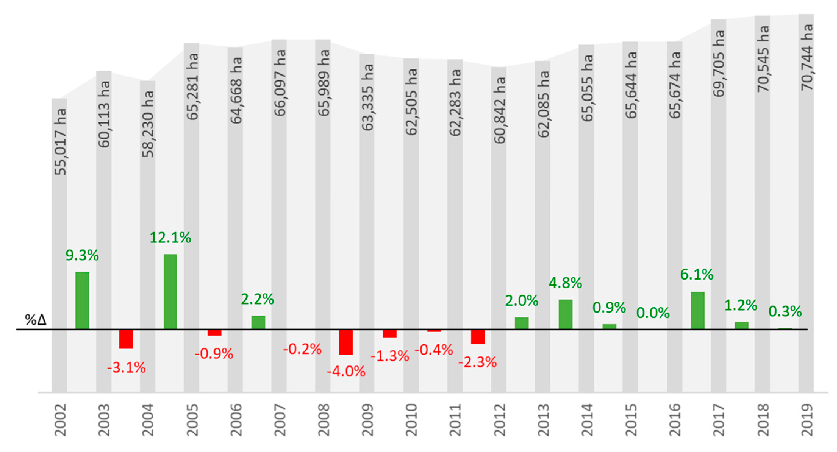
Figure 3.
Distribution of the crop area under greenhouse in 2019 for the (a) Spanish Autonomous Communities and (b) Andalusian provinces [2].
Figure 3.
Distribution of the crop area under greenhouse in 2019 for the (a) Spanish Autonomous Communities and (b) Andalusian provinces [2].

Figure 4.
Multi-span or multi-tunnel greenhouse on an irregularly-shaped plot [24].
Figure 4.
Multi-span or multi-tunnel greenhouse on an irregularly-shaped plot [24].
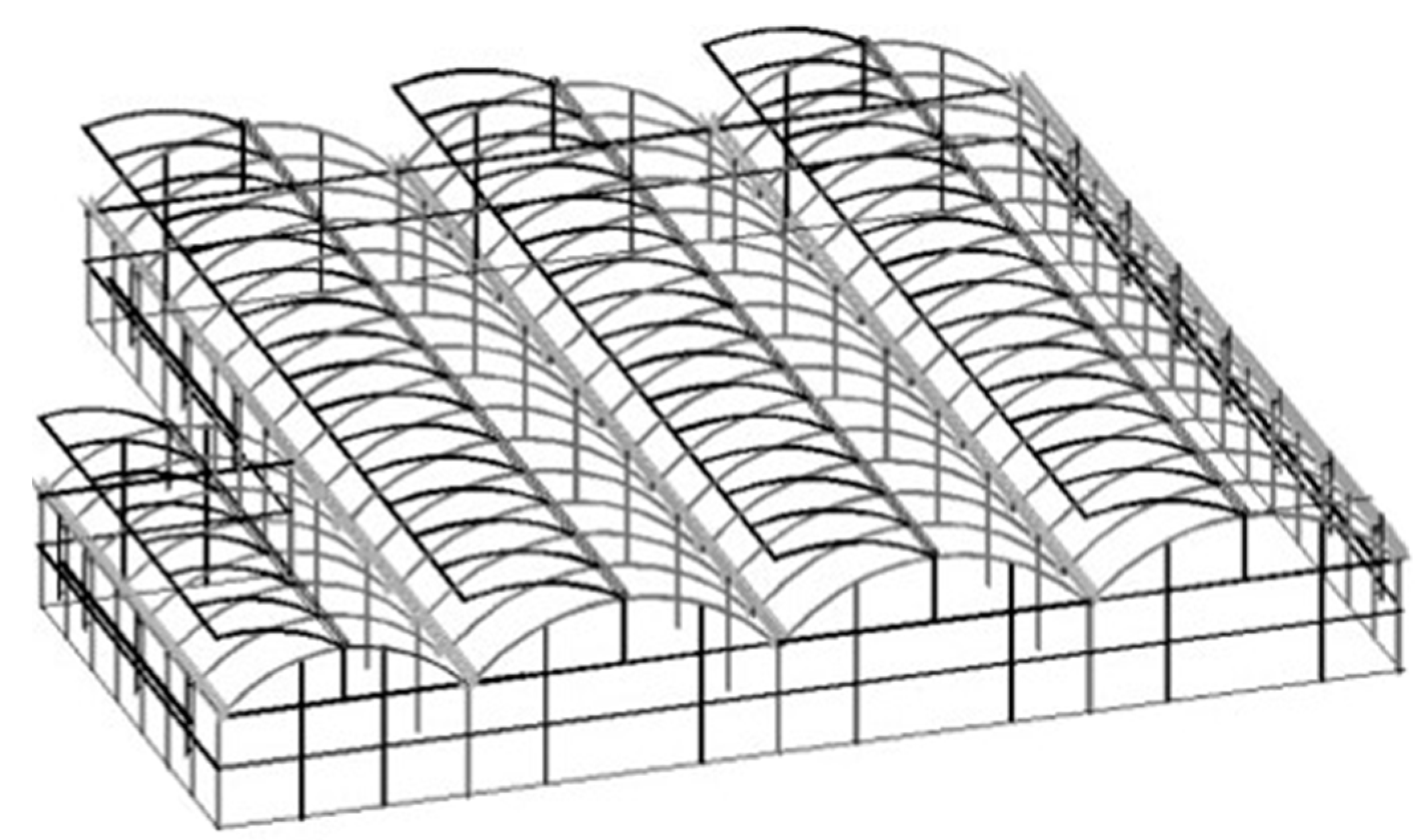
Figure 5.
Typical greenhouse structure (adapted from Vázquez-Cabrera et al. [48] and Iribarne et al. [24]).

Figure 6.
Symmetry planes and dimensions of the studied greenhouse model.

Figure 7.
Codification of the different nodes in the greenhouse structure.

Figure 8.
Close-up details of the nodes indicated in Figure 7.
Figure 8.
Close-up details of the nodes indicated in Figure 7.

Figure 9.
0°-wind load values according to EN 13031-1 [53].
Figure 9.
0°-wind load values according to EN 13031-1 [53].

Figure 10.
90°-wind load values according to EN 13031-1 [53].
Figure 10.
90°-wind load values according to EN 13031-1 [53].
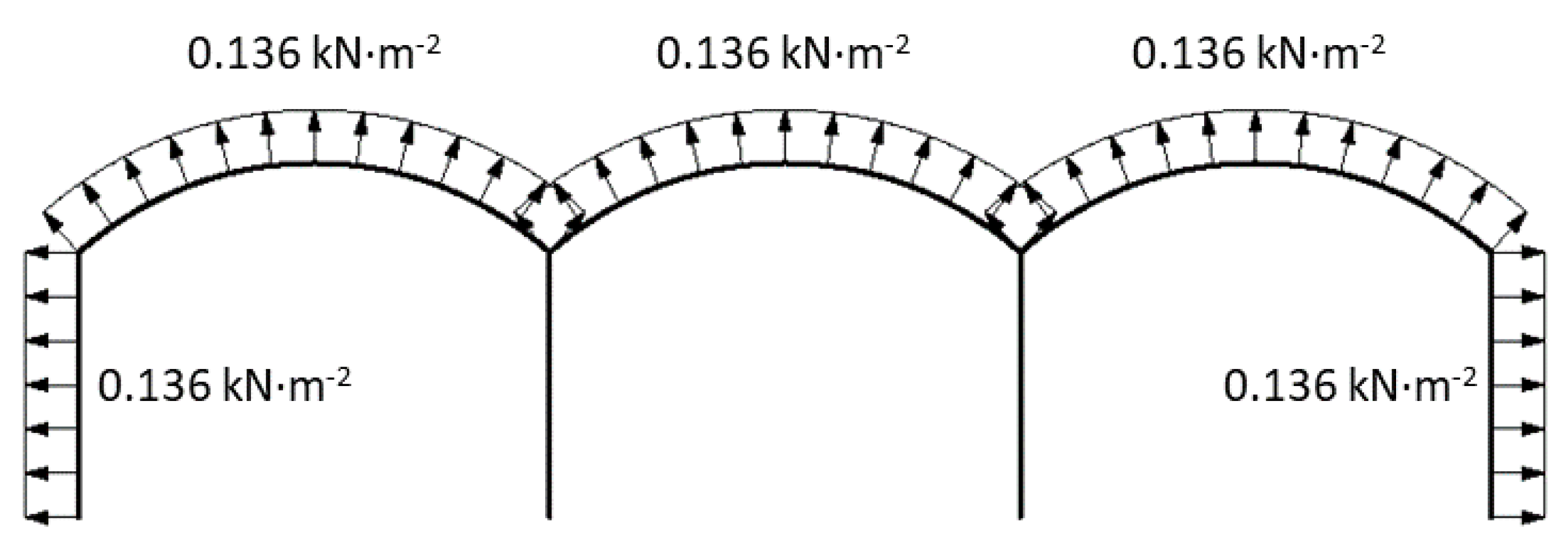
Figure 11.
Mesh distribution for (a) the even-span greenhouse (EV-D22) defined in Kim et al. [44]; and (b) the multi-span greenhouse.
Figure 11.
Mesh distribution for (a) the even-span greenhouse (EV-D22) defined in Kim et al. [44]; and (b) the multi-span greenhouse.

Figure 12.
(a) Wind velocity vertical profile and (b) turbulence for a terrain category II according to the Eurocode 1-4 [57].
Figure 12.
(a) Wind velocity vertical profile and (b) turbulence for a terrain category II according to the Eurocode 1-4 [57].

Figure 13.
(a) Concrete footing design with the height comprised of four horizontal divisions. (b) Close-up view of a subdivision.
Figure 13.
(a) Concrete footing design with the height comprised of four horizontal divisions. (b) Close-up view of a subdivision.

Figure 14.
Finite element model for a concrete footing: (a) mesh and (b) stress lines in the plane of symmetry.
Figure 14.
Finite element model for a concrete footing: (a) mesh and (b) stress lines in the plane of symmetry.

Figure 15.
Vertical deformations, expressed in meters, employed to adjust the modulus of elasticity and the subgrade reaction modulus.
Figure 15.
Vertical deformations, expressed in meters, employed to adjust the modulus of elasticity and the subgrade reaction modulus.
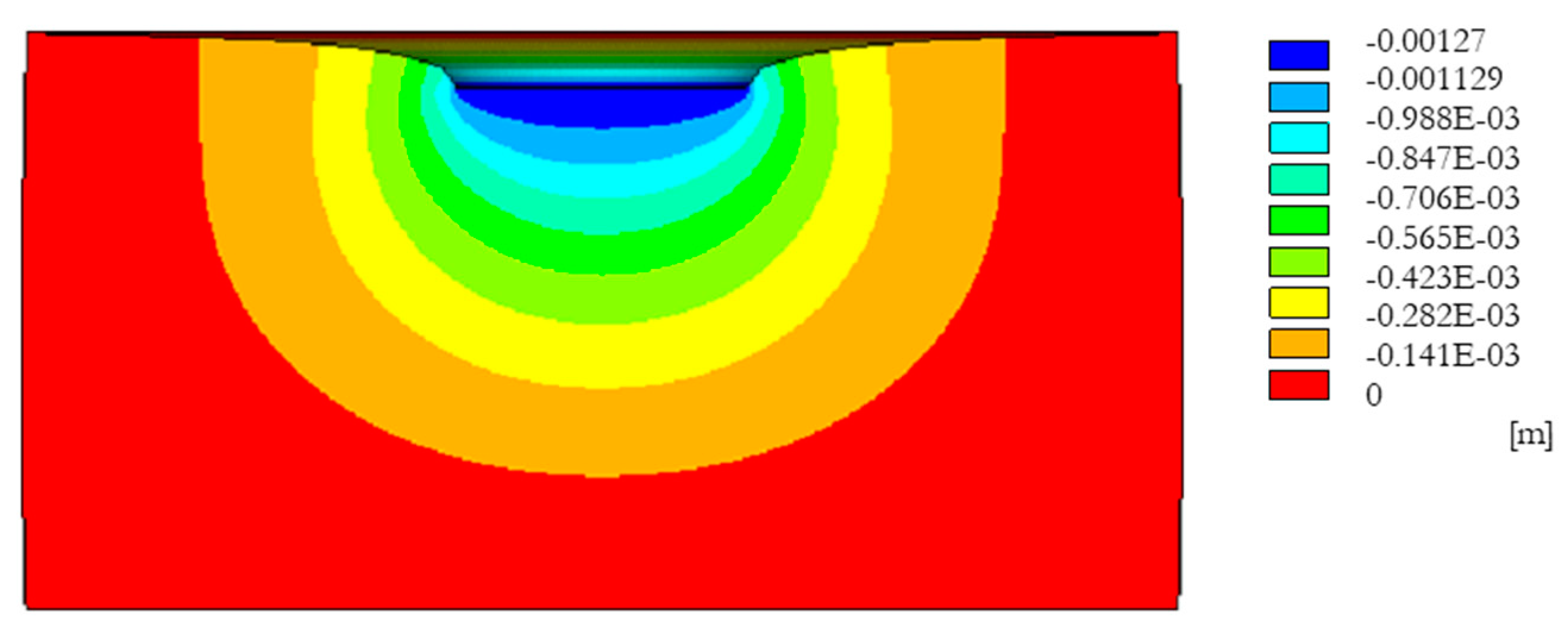
Figure 16.
Wind external pressure coefficient values for the 22° even span greenhouse determined by the computational fluid dynamics (CFD) model simulation and the wind tunnel experiments.
Figure 16.
Wind external pressure coefficient values for the 22° even span greenhouse determined by the computational fluid dynamics (CFD) model simulation and the wind tunnel experiments.

Figure 17.
Wind velocity on the streamlines.
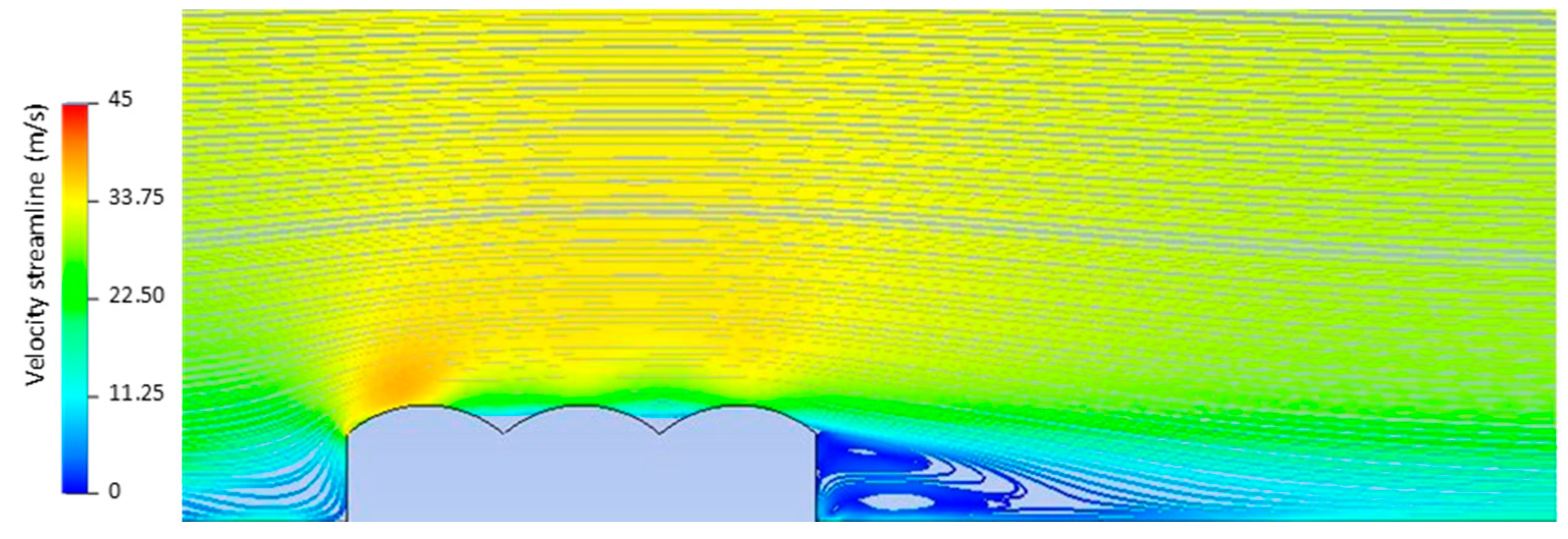
Figure 18.
Wind external pressure coefficients determined through CFD for the multi-tunnel greenhouse: (a) roof; (b) left lateral column; (c) right lateral column.
Figure 18.
Wind external pressure coefficients determined through CFD for the multi-tunnel greenhouse: (a) roof; (b) left lateral column; (c) right lateral column.

Figure 19.
0° wind load values determined by CFD.

Figure 20.
Buckling mode for (a) load combination 1 based on wind loads according to EN 13031-1 (2001) (first arch, up-down displacement type) and (b) load combination 1CFD based on wind loads calculated through CFD (first arch, down-up displacement type).
Figure 20.
Buckling mode for (a) load combination 1 based on wind loads according to EN 13031-1 (2001) (first arch, up-down displacement type) and (b) load combination 1CFD based on wind loads calculated through CFD (first arch, down-up displacement type).
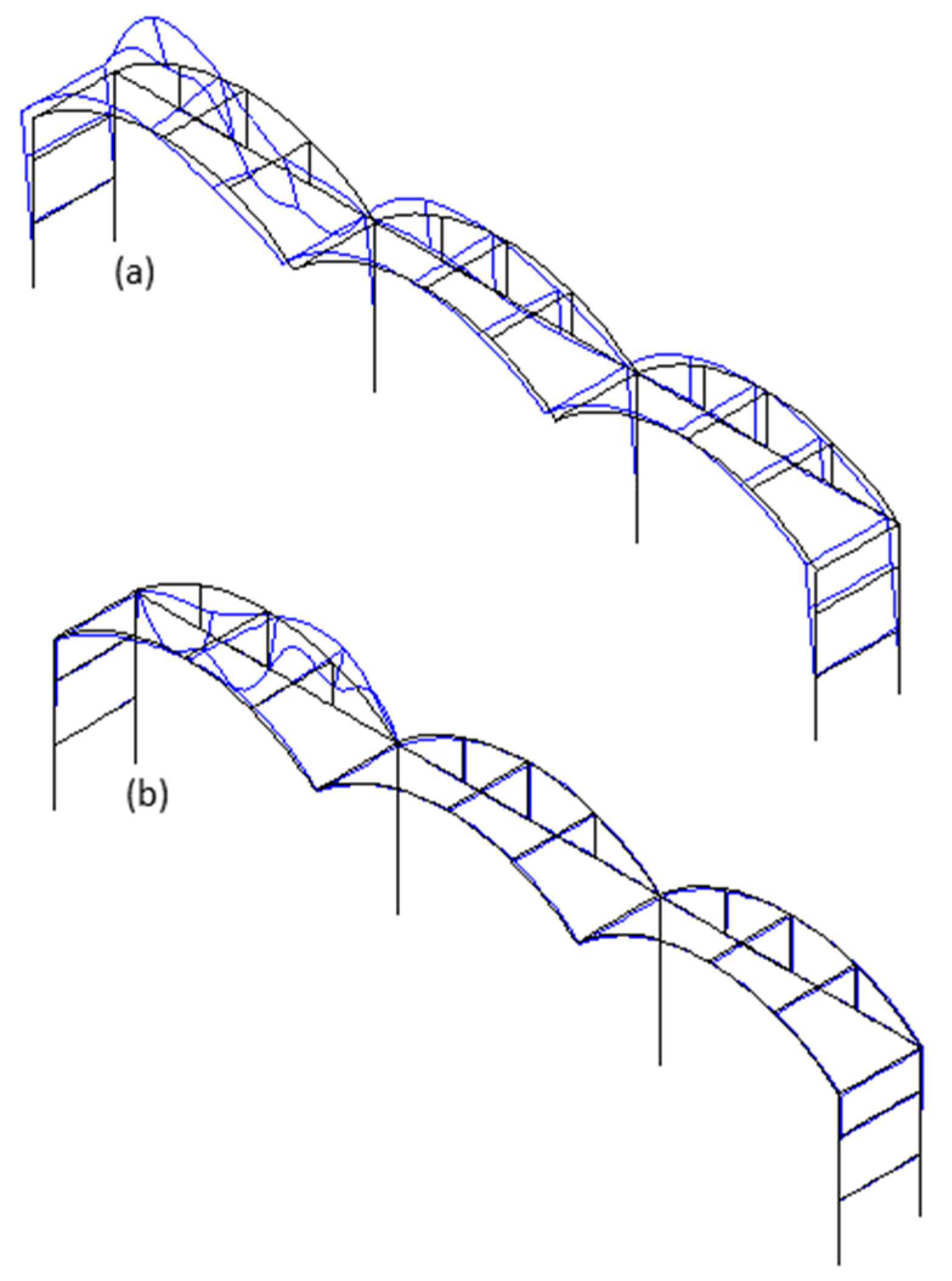
Figure 21.
Buckling mode for (a) load combination 2 based on wind loads according to EN 13031-1 (2001) (first arch, up-down displacement type) and (b) load combination 2CFD based on wind loads calculated through CFD (first arch, down-up displacement type).
Figure 21.
Buckling mode for (a) load combination 2 based on wind loads according to EN 13031-1 (2001) (first arch, up-down displacement type) and (b) load combination 2CFD based on wind loads calculated through CFD (first arch, down-up displacement type).
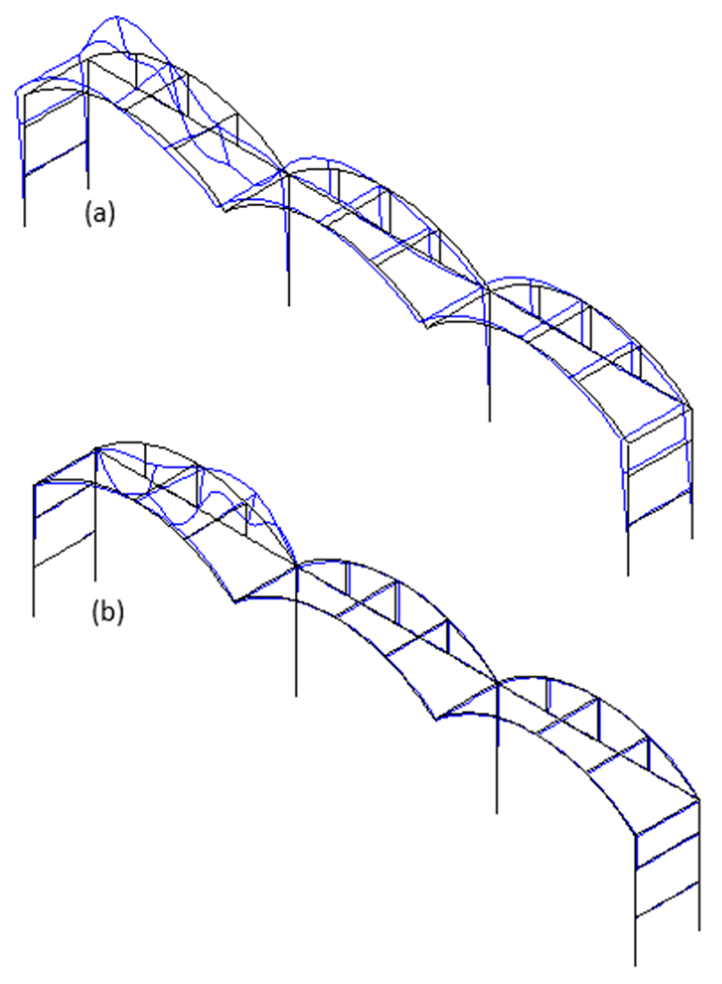
Figure 22.
Buckling mode for (a) load combination 7 based on wind loads according to EN 13031-1 (2001) (general type) and (b) load combination 7CFD based on wind loads calculated through CFD (first arch, up-down displacement type).
Figure 22.
Buckling mode for (a) load combination 7 based on wind loads according to EN 13031-1 (2001) (general type) and (b) load combination 7CFD based on wind loads calculated through CFD (first arch, up-down displacement type).

Figure 23.
Pressures in the plane of symmetry, expressed in kN·m−2 and determined by the Finite Element Model and the Matrix Model, on the base of the footing due to a 7.58 kN axial load and the footing self-weight.
Figure 23.
Pressures in the plane of symmetry, expressed in kN·m−2 and determined by the Finite Element Model and the Matrix Model, on the base of the footing due to a 7.58 kN axial load and the footing self-weight.
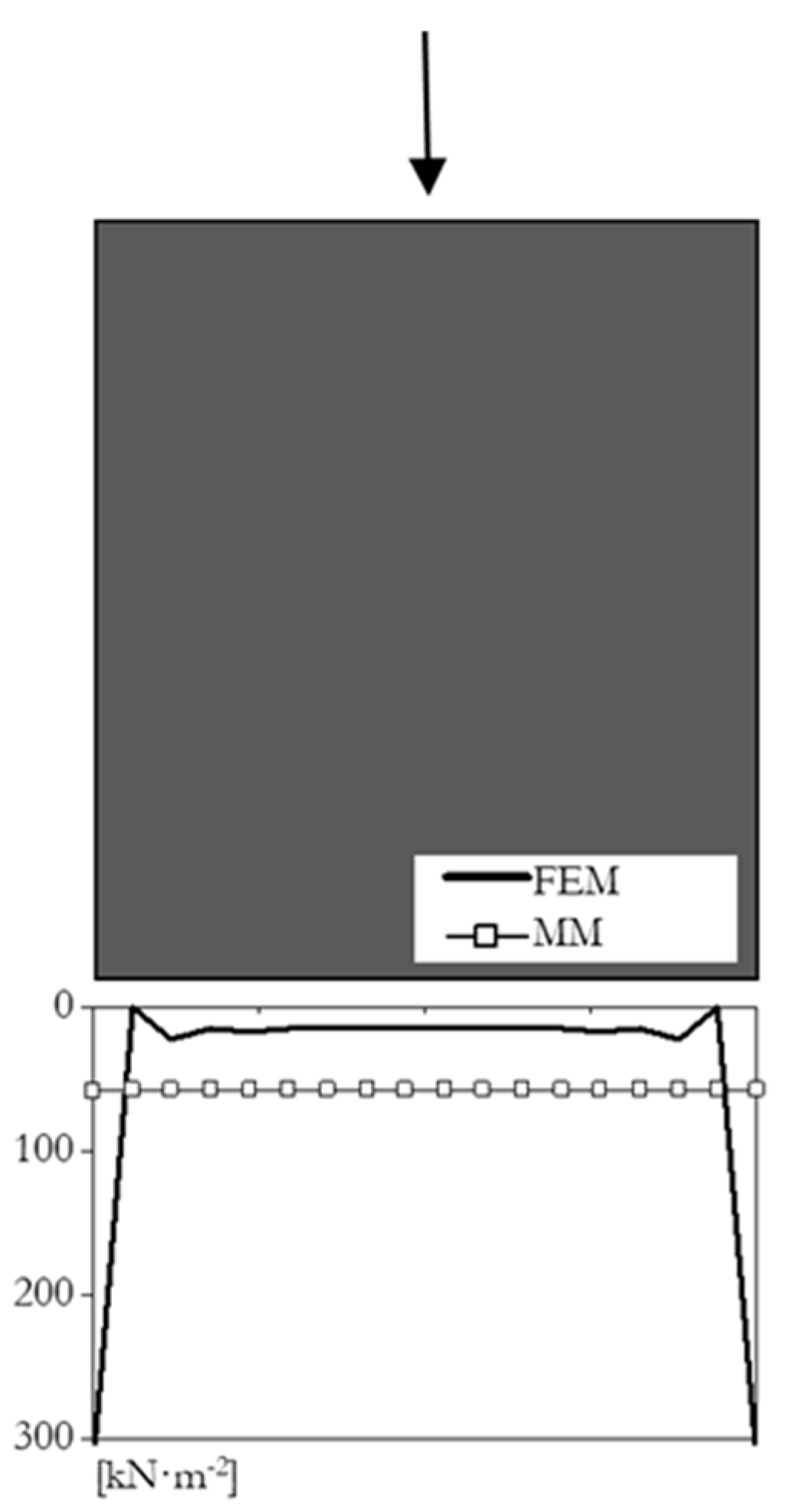
Figure 24.
Pressure in the plane of symmetry, expressed in kN·m−2 and determined by the Finite Element Model and the Matrix Model, on the walls and base of the footing due to a 2.61 kN shear load.
Figure 24.
Pressure in the plane of symmetry, expressed in kN·m−2 and determined by the Finite Element Model and the Matrix Model, on the walls and base of the footing due to a 2.61 kN shear load.

Figure 25.
Pressure in the plane of symmetry, expressed in kN·m−2 and determined by the Finite Element Model and the Matrix Model, on the walls and base of the footing due to a 5.53 kN·m moment load.
Figure 25.
Pressure in the plane of symmetry, expressed in kN·m−2 and determined by the Finite Element Model and the Matrix Model, on the walls and base of the footing due to a 5.53 kN·m moment load.

Figure 26.
Pressure in the plane of symmetry, expressed in kN·m−2 and determined by the Finite Element Model and the Matrix Model, on the walls and base of the footing due to the simultaneous application of axial, shear and moment stresses.
Figure 26.
Pressure in the plane of symmetry, expressed in kN·m−2 and determined by the Finite Element Model and the Matrix Model, on the walls and base of the footing due to the simultaneous application of axial, shear and moment stresses.

Figure 27.
(a) Horizontal and (b) vertical deformations in the plane of symmetry, expressed in m, due to the simultaneous application of N, V and M stresses determined through FEM.
Figure 27.
(a) Horizontal and (b) vertical deformations in the plane of symmetry, expressed in m, due to the simultaneous application of N, V and M stresses determined through FEM.


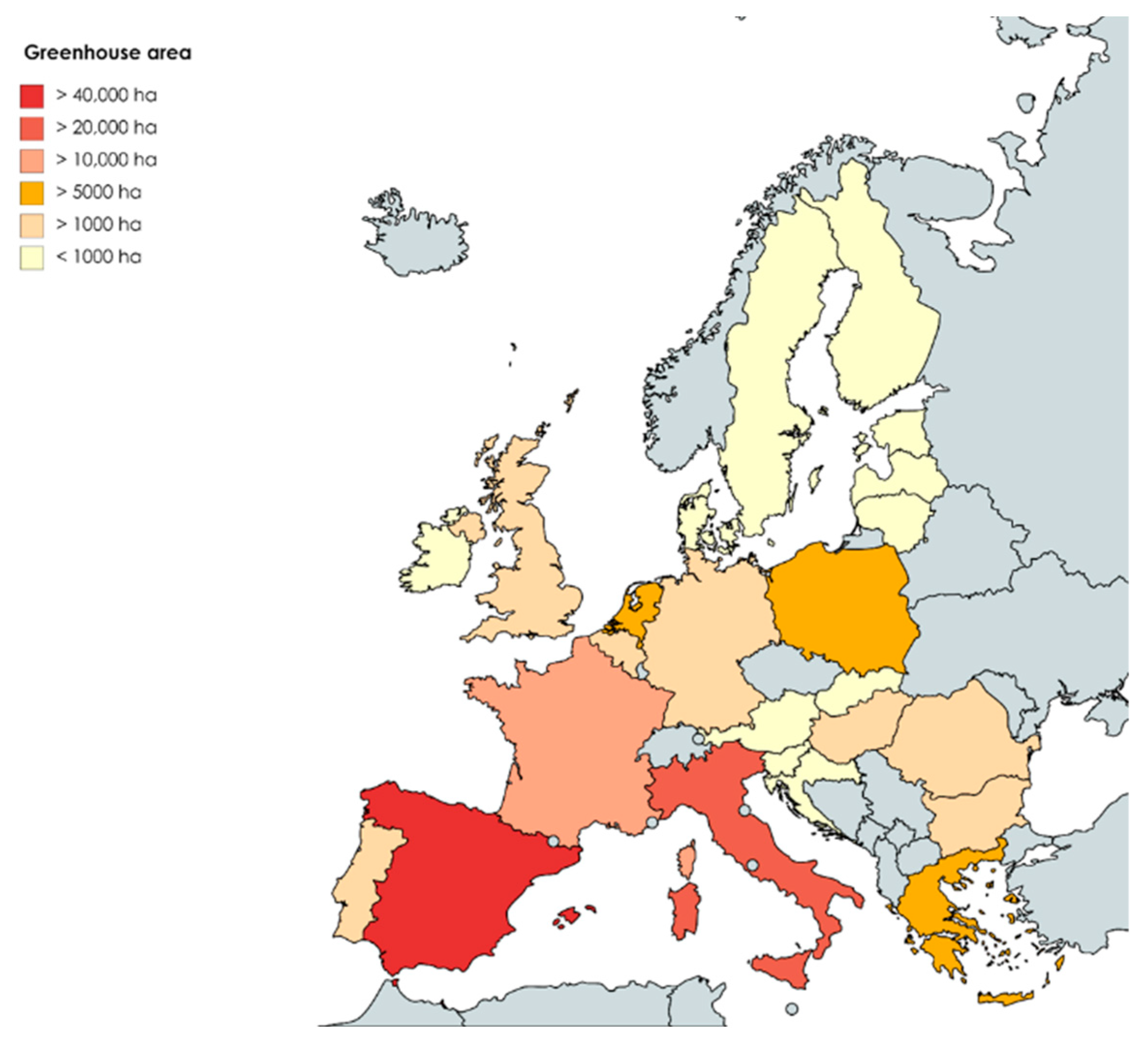
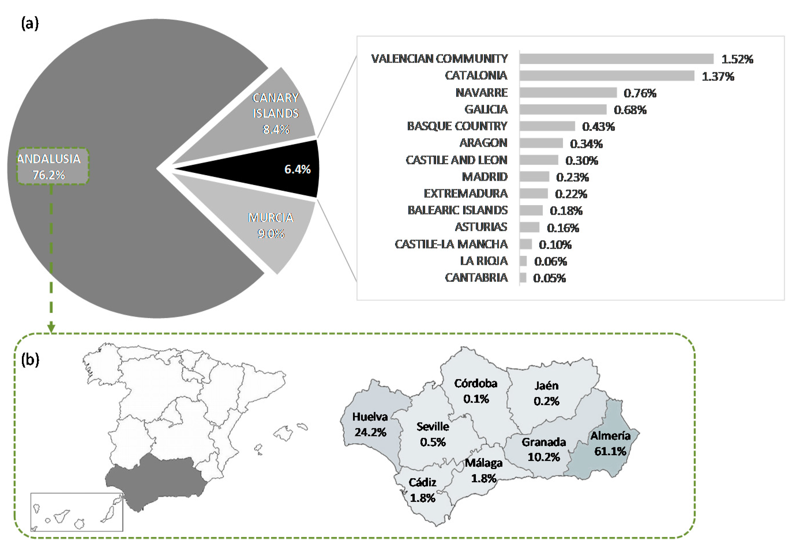
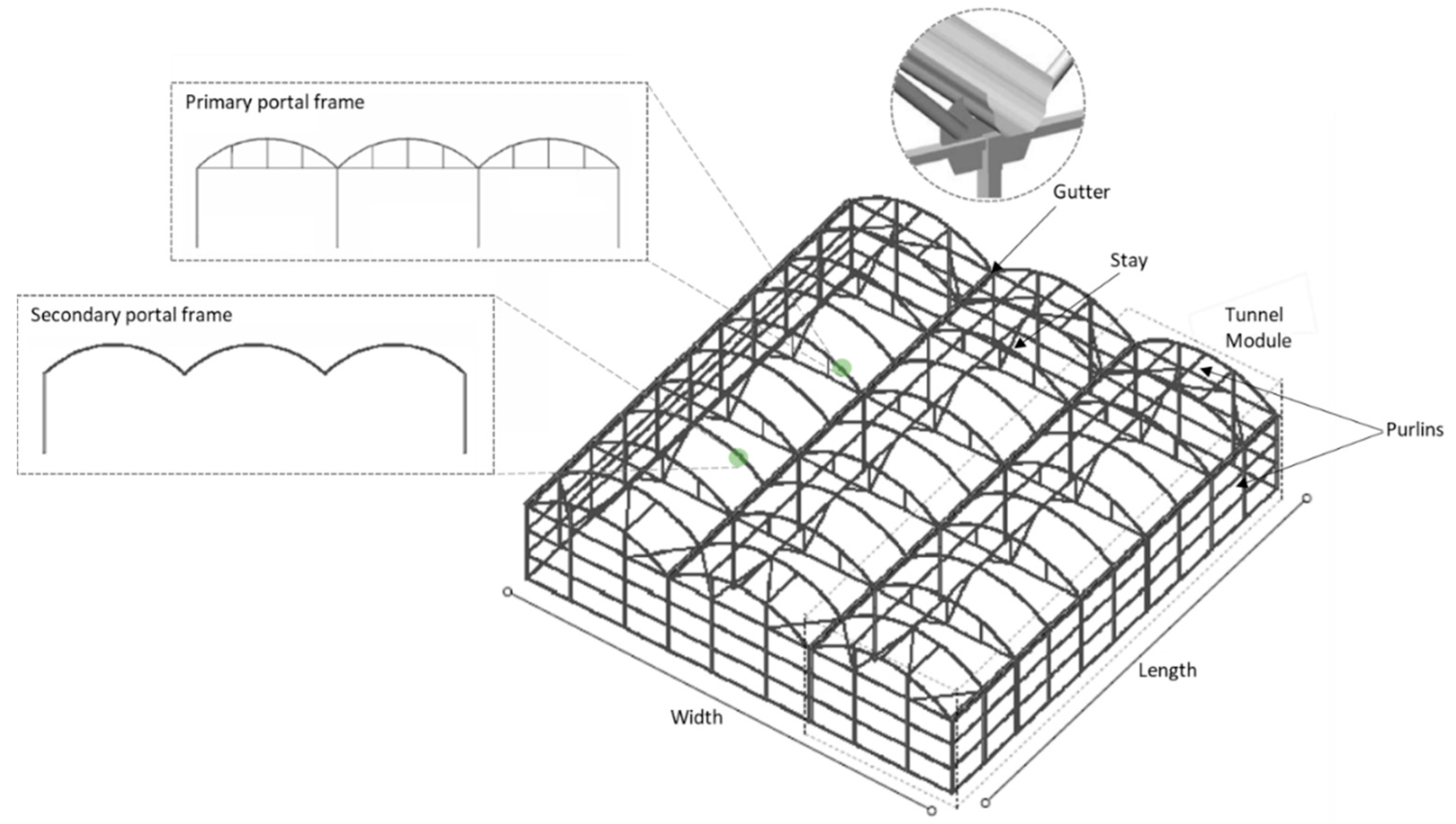
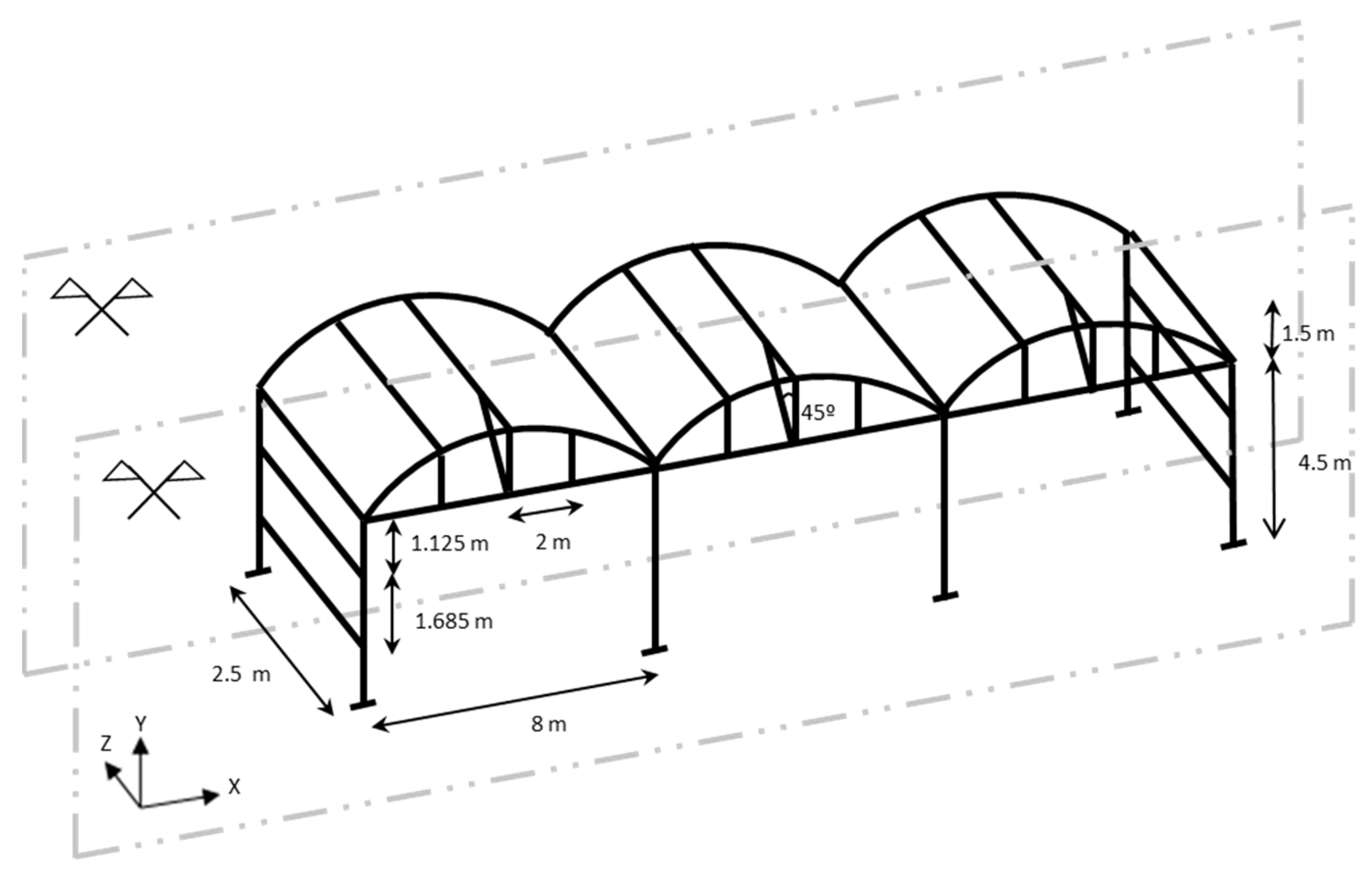
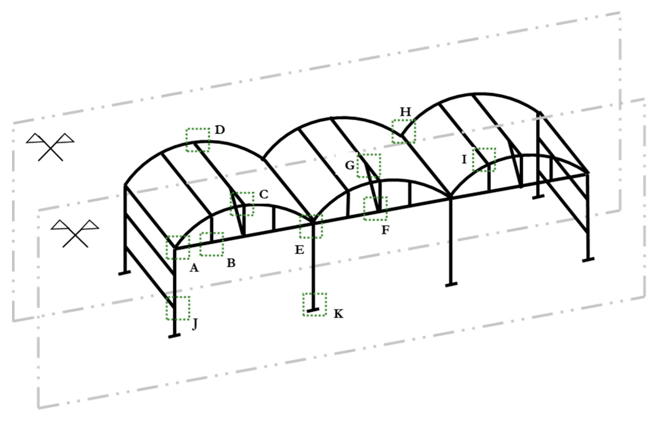
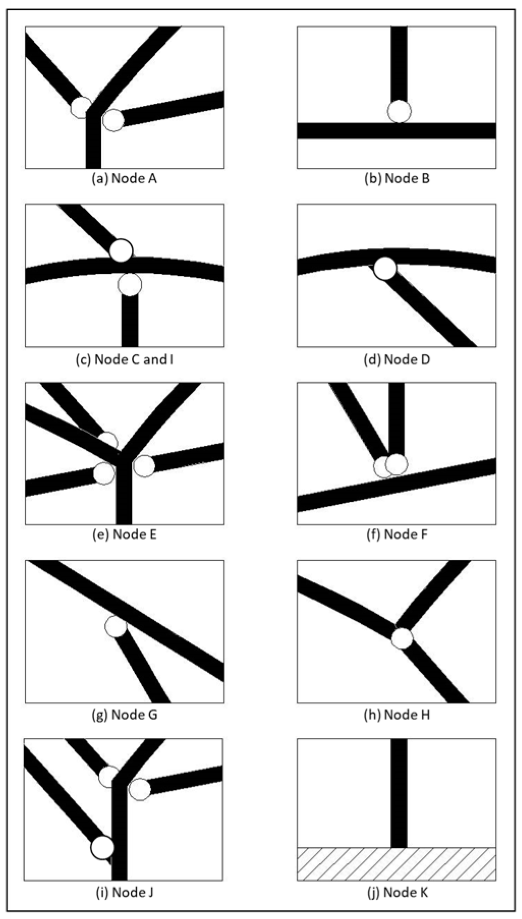
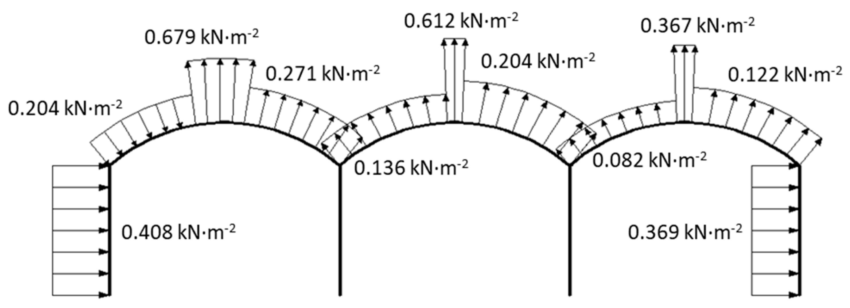
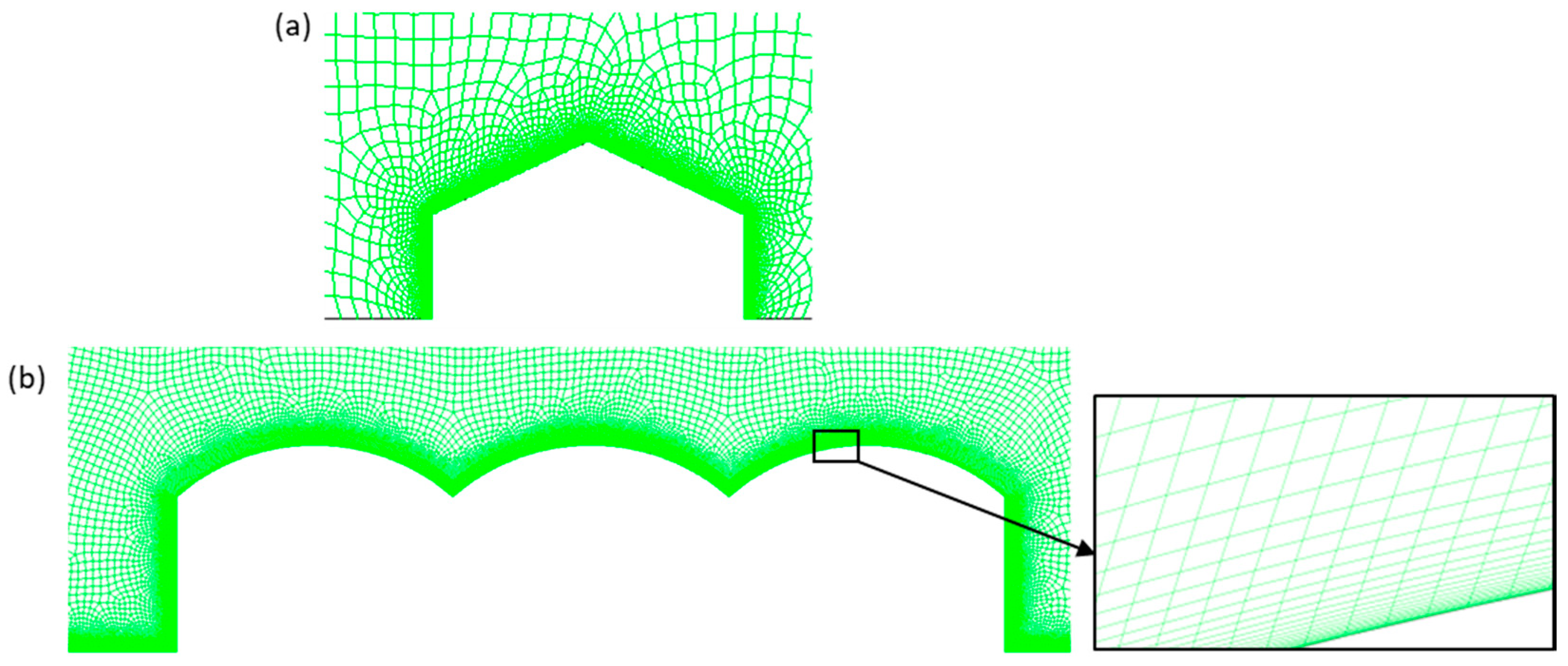
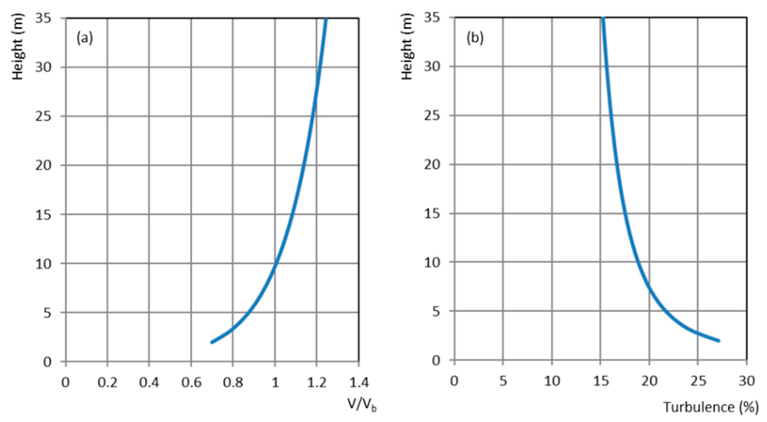
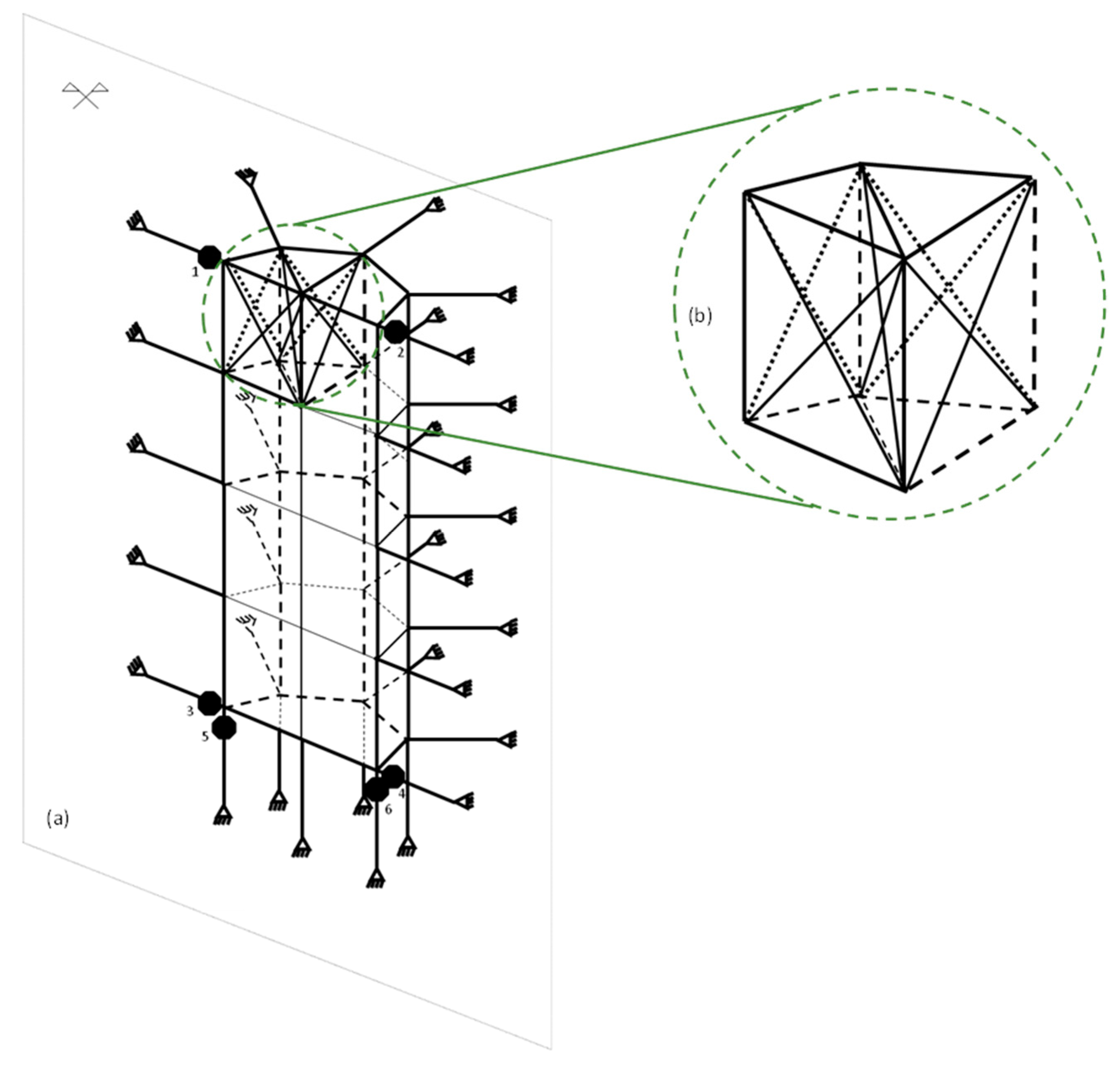
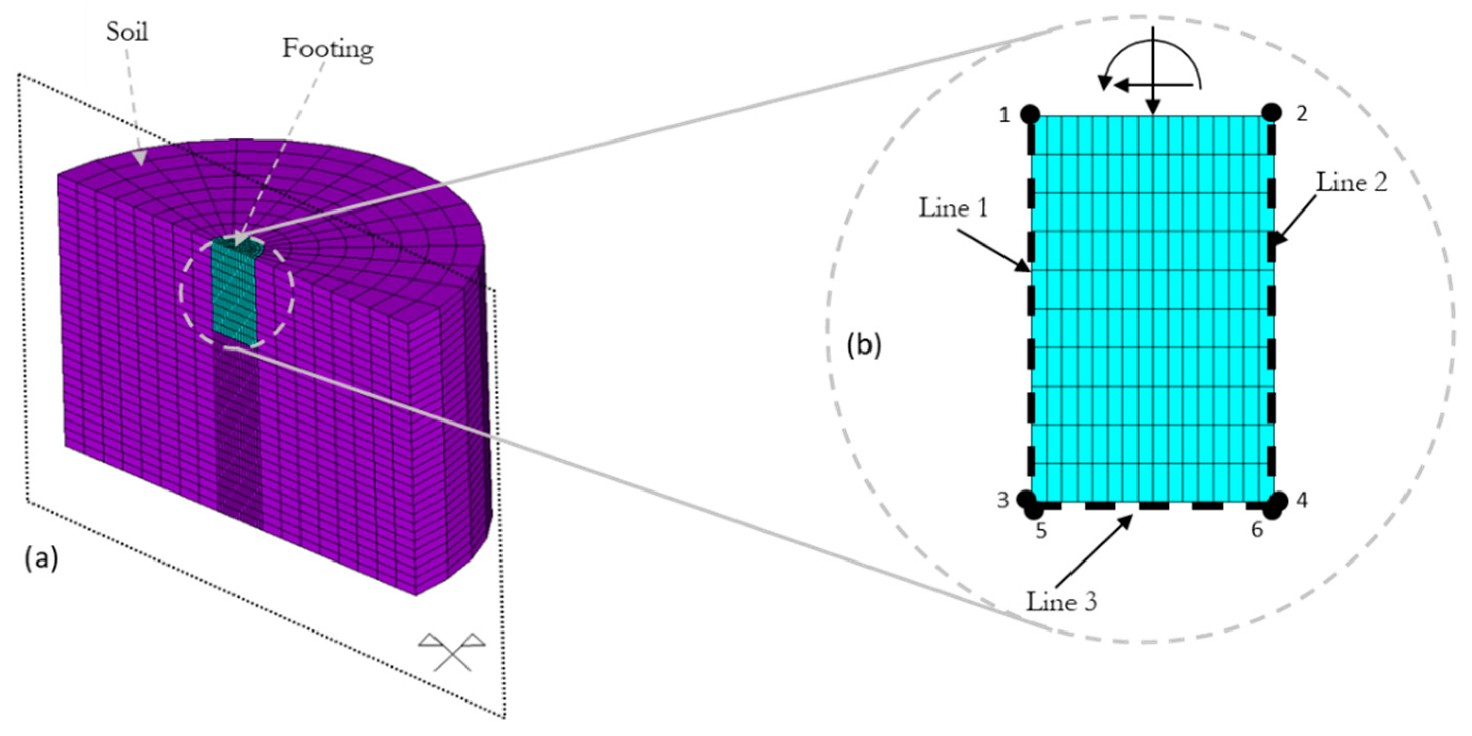
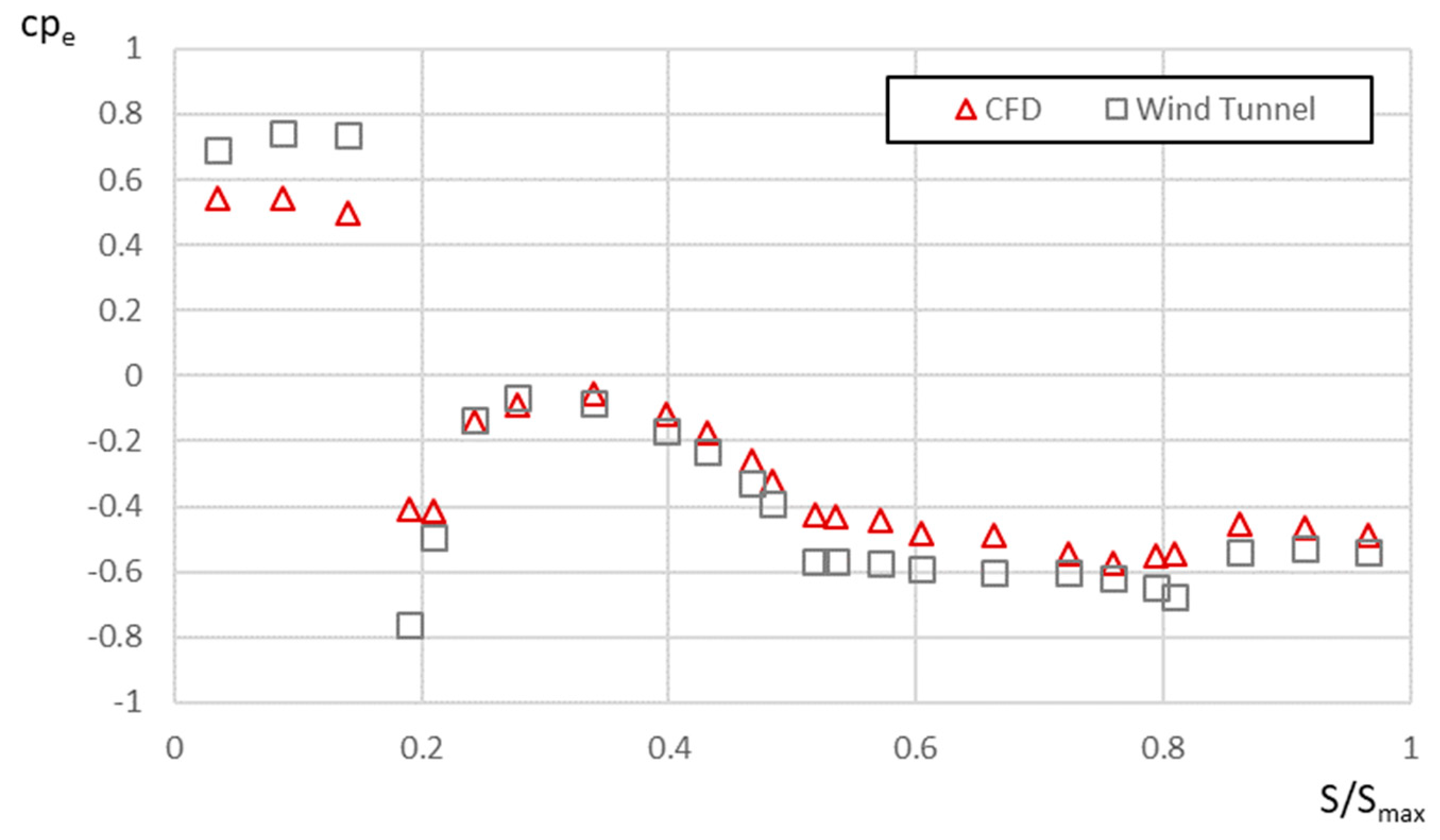
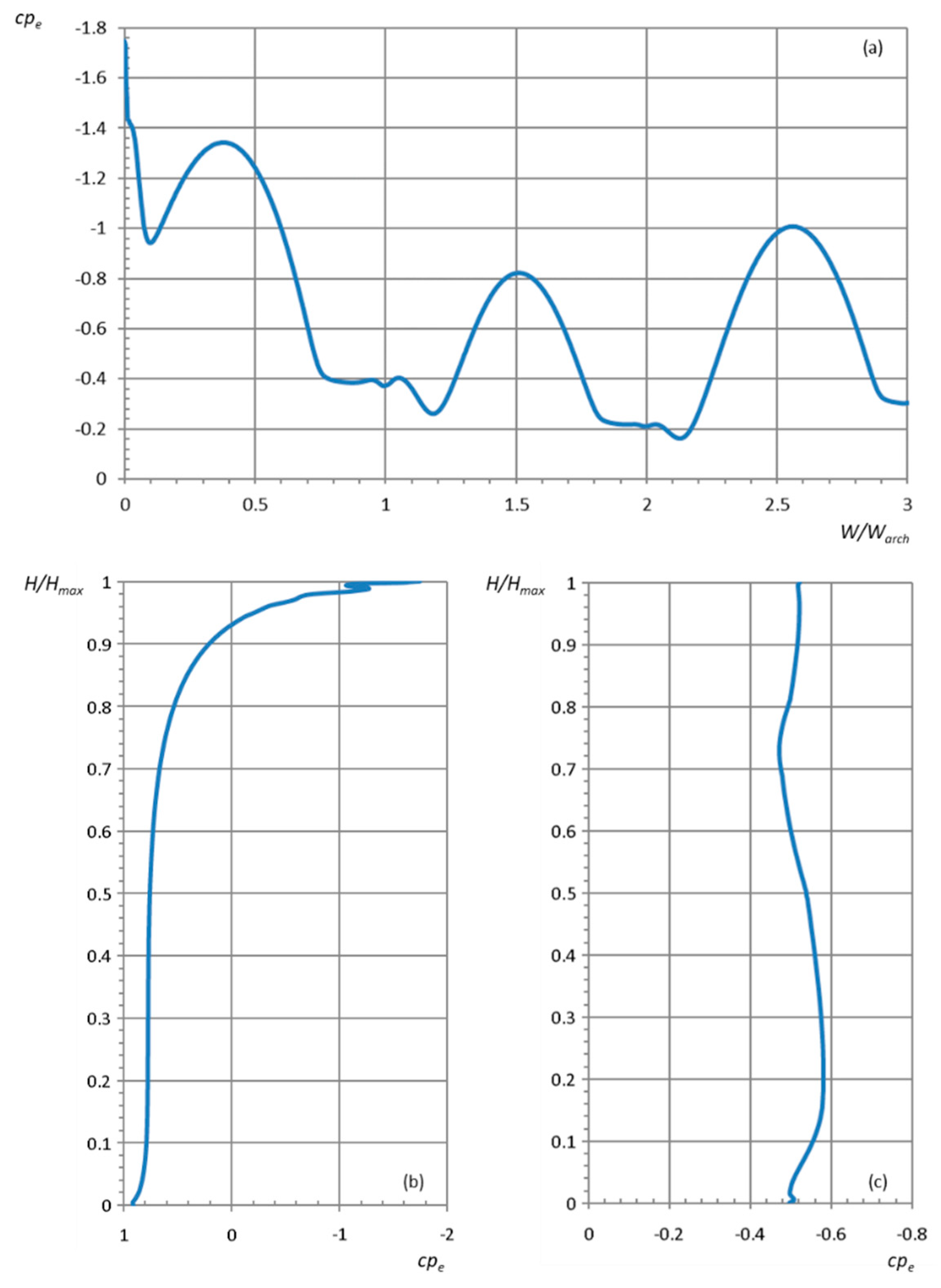
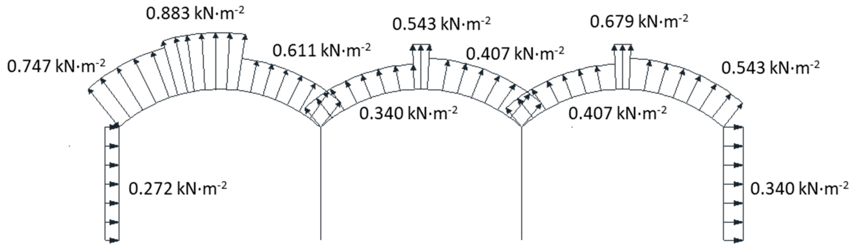
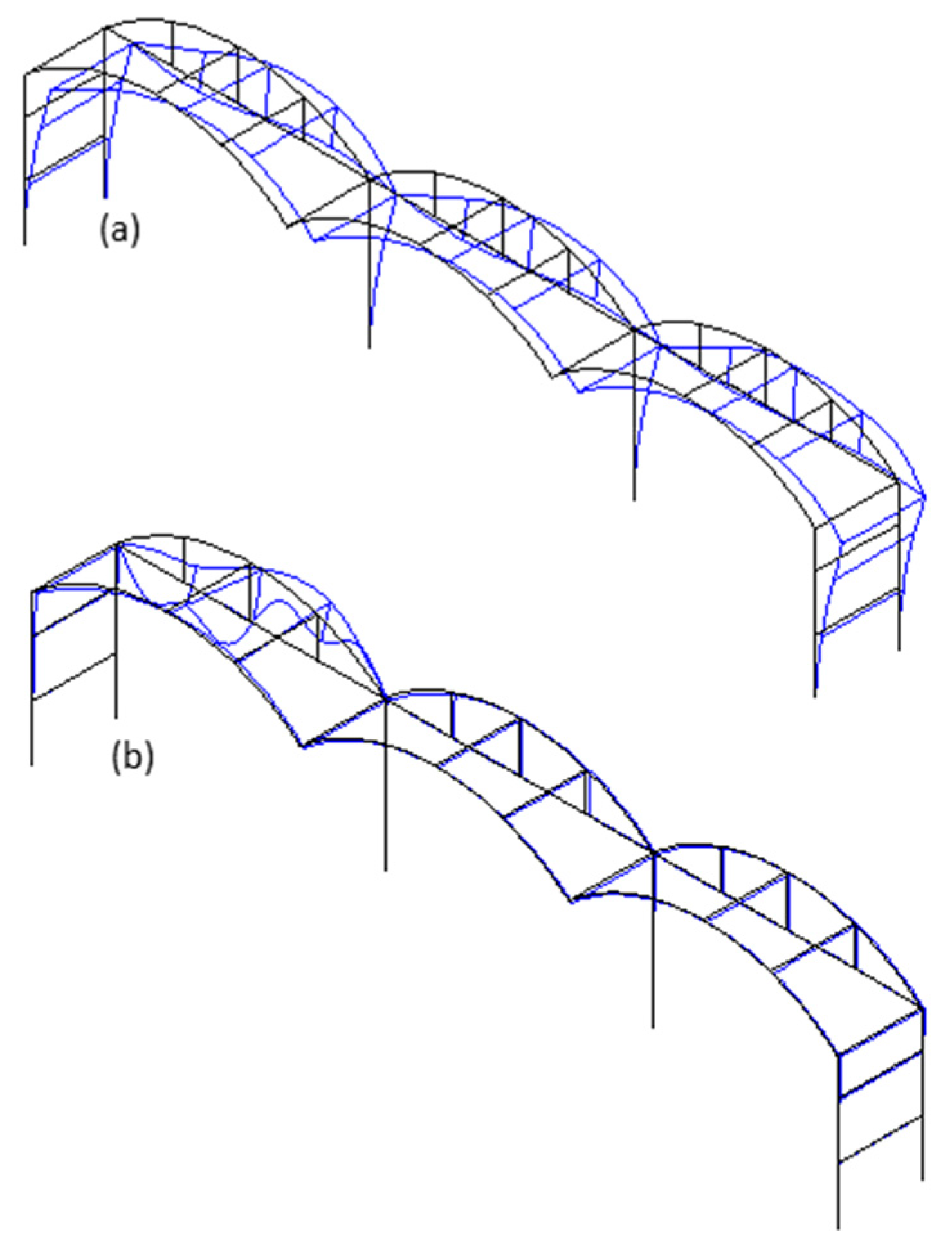
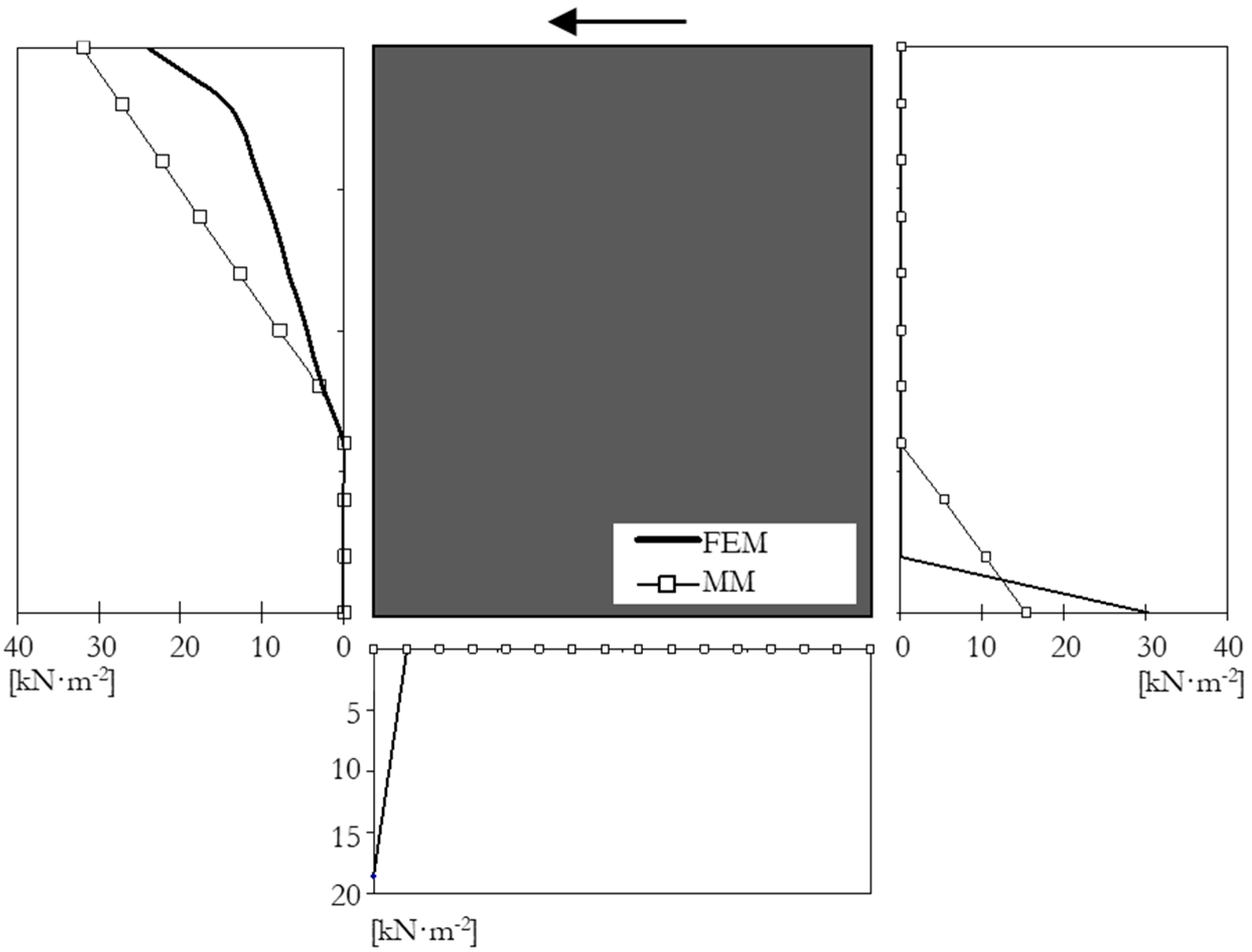
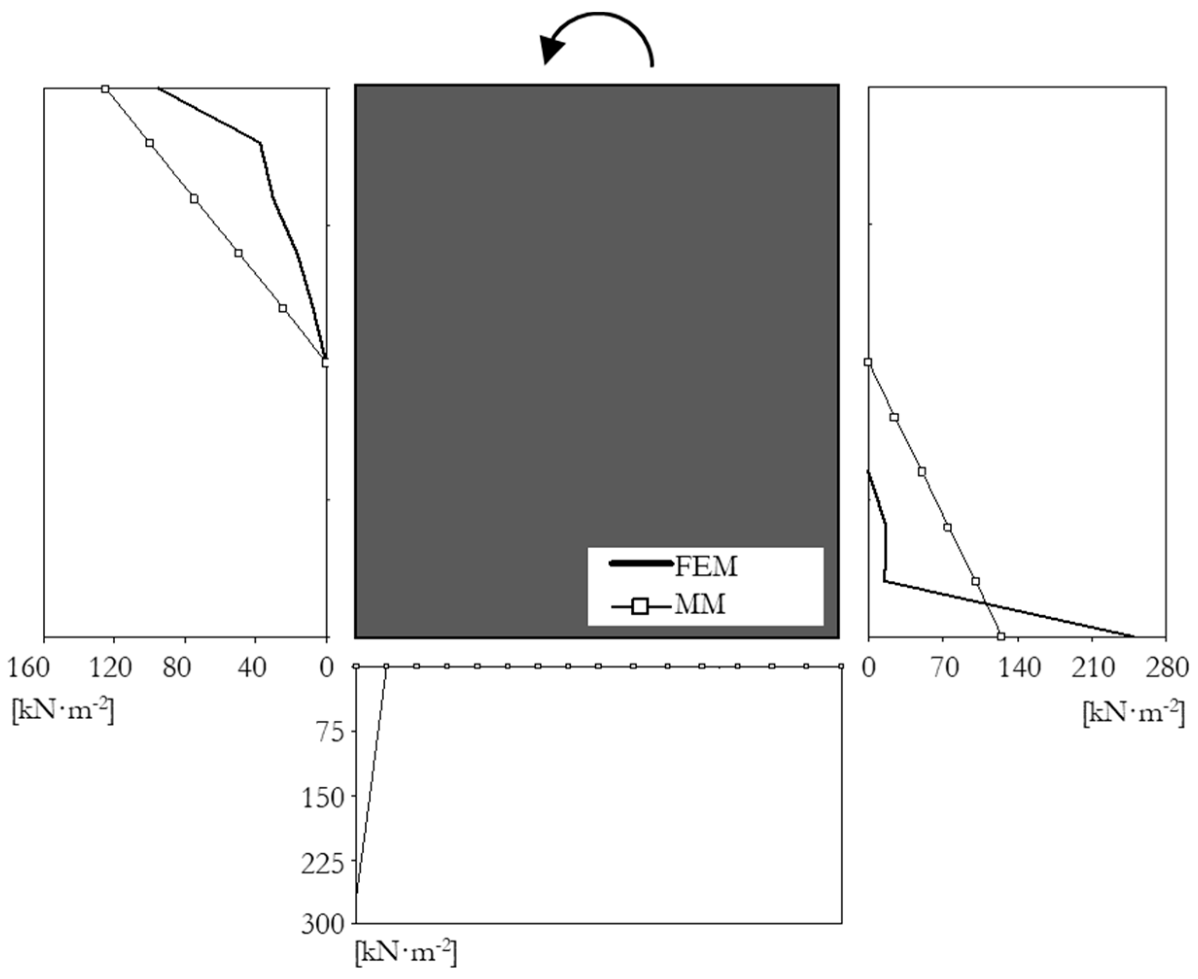
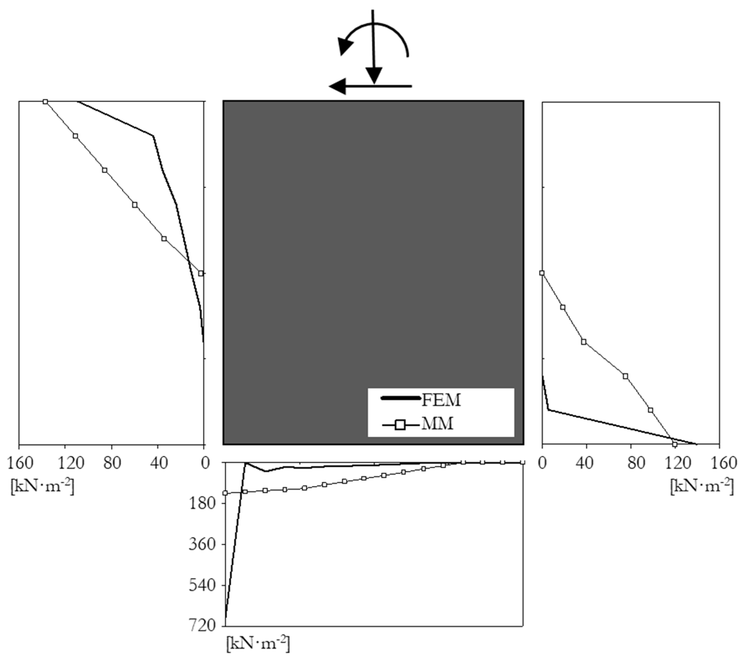
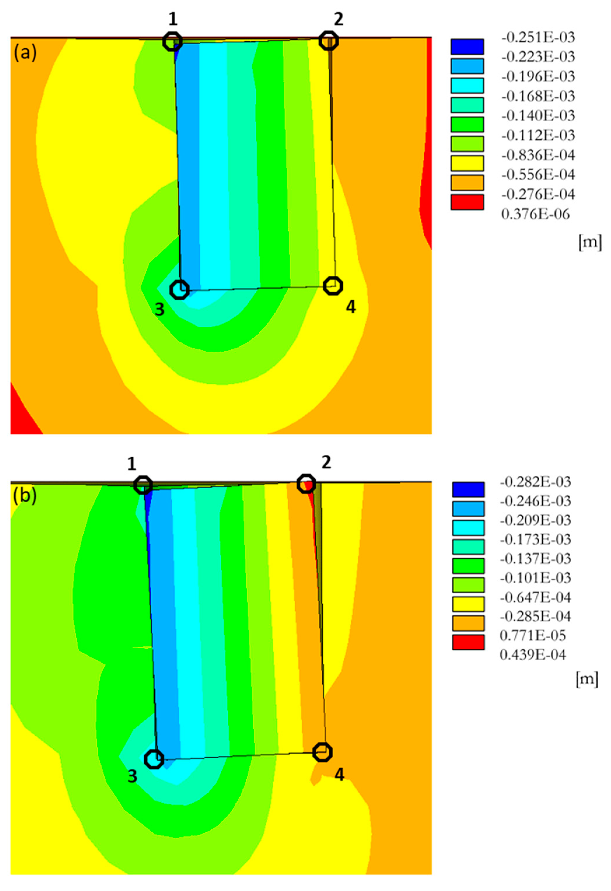
Table 1.
External pressure coefficient and wind load values for 0° and 90° wind directions.
| Wind Direction | Part of the Greenhouse | Angle (°) | External Pressure Coefficient (cpe) | Load (kN·m−2) |
|---|---|---|---|---|
| 0° | First tunnel | 0–55 | 0.30 | 0.204 |
| 55–70 | −1.00 | −0.679 | ||
| 70–115 | −1.00 | −0.679 | ||
| 115–gutter | −0.40 | −0.271 | ||
| Second tunnel | 0–80 | −0.20 | −0.136 | |
| 80–100 | −0.90 | −0.612 | ||
| 100–gutter | −0.30 | −0.204 | ||
| Third tunnel | 0–80 | −0.12 | −0.082 | |
| 80–100 | −0.54 | −0.367 | ||
| 100–gutter | −0.18 | −0.122 | ||
| Left wall | - | 0.60 | 0.408 | |
| Right wall | - | −0.50 | −0.369 | |
| 90° | All | - | −0.20 | −0.136 |
Table 2.
External pressure coefficient and wind load values for 0° and 90° wind directions.
| Load Combination | |||||
|---|---|---|---|---|---|
| 1 | 1.2 · Permanent load | + | 1.2 · 0° wind load | + | 1.2 · 1 · crop load |
| 2 | 1 · Permanent load | + | 1.2 · 0° wind load | + | 1.2 · 1 · crop load |
| 3 | 1.2 · Permanent load | + | 1.2 · 90° wind load | + | 1.2 · 1 · crop load |
| 4 | 1 · Permanent load | + | 1.2 · 90° wind load | + | 1.2 · 1 · crop load |
| 5 | 1.2 · Permanent load | + | 1.2 · 1 · crop load | ||
| 6 | 1 · Permanent load | + | 1.2 · 1 · crop load | ||
| 7 | 1.2 · Permanent load | + | 1.2 · 0.6 · 0° wind load | + | 1.2 · 1 · crop load |
| 8 | 1 · Permanent load | + | 1.2 · 0.6 · 0° wind load | + | 1.2 · 1 · crop load |
| 9 | 1.2 · Permanent load | + | 1.2 · 0.6 · 90° wind load | + | 1.2 · 1 · crop load |
| 10 | 1 · Permanent load | + | 1.2 · 0.6 · 90° wind load | + | 1.2 · 1 · crop load |
| 11 | 1.2 · Permanent load | + | 1.2 · 0° wind load | ||
| 12 | 1 · Permanent load | + | 1.2 · 0° wind load | ||
| 13 | 1.2 · Permanent load | + | 1.2 · 90° wind load | ||
| 14 | 1 · Permanent load | + | 1.2 · 90° wind load | ||
| 15 | 1.2 · Permanent load | + | 1.2 · 1 · crop load | + | 1.2 · concentrated vertical action |
| 16 | 1 · Permanent load | + | 1.2 · 1 · crop load | + | 1.2 · concentrated vertical action |
| 17 | 1.2 · Permanent load | ||||
| 18 | 1 · Permanent load | ||||
| 19 | 1.2 · Permanent load | + | 1.2 · 1 · crop load | + | 0.8 · accidental snow load |
| 20 | 1 · Permanent load | + | 1.2 · 1 · crop load | + | 0.8 · accidental snow load |
Table 3.
Wind load values at 0°-direction estimated by CFD.
| Wind Direction | Part of the Greenhouse | Angle (°) | External Pressure Coefficient (cpe) | Load (kN·m−2) |
|---|---|---|---|---|
| 0° | First tunnel | 0–55 | −1.20 | −0.747 |
| 55–70 | −1.30 | −0.883 | ||
| 70–115 | −1.30 | −0.883 | ||
| 115–gutter | −0.90 | −0.611 | ||
| Second tunnel | 0–80 | −0.50 | −0.340 | |
| 80–100 | −0.80 | −0.543 | ||
| 100–gutter | −0.60 | −0.407 | ||
| Third tunnel | 0–80 | −0.60 | −0.407 | |
| 80–100 | −1.00 | −0.679 | ||
| 100–gutter | −0.80 | −0.543 | ||
| Left wall | - | 0.40 | 0.272 | |
| Right wall | - | −0.50 | −0.340 |
Table 4.
λcr values for the different combinations considered.
| Load Combination | λcr | Buckling Mode Shape |
|---|---|---|
| 1 | 8.12 | First arch, up-down displacement |
| 1CFD | 3.5 | First arch, down-up displacement |
| 2 | 7.94 | First arch, up-down displacement |
| 2CFD | 3.46 | First arch, down-up displacement |
| 3 | 18.6 | General |
| 4 | 20.1 | General |
| 5 | 6.34 | General |
| 6 | 6.56 | General |
| 7 | 11.87 | General |
| 7CFD | 8.12 | First arch, down-up displacement |
| 8 | 12.52 | General |
| 8CFD | 7.91 | First arch, down-up displacement |
| 9 | 10.83 | General |
| 10 | 11.46 | General |
| 11 | 4.63 | First arch, down-up displacement |
| 11CFD | 2.59 | First arch, down-up displacement |
| 12 | 4.56 | First arch, down-up displacement |
| 12CFD | 2.56 | First arch, down-up displacement |
| 13 | 26.88 | Almost local, central arch |
| 14 | 26.14 | Almost local, first arch |
| 15 | 5.8 | General |
| 16 | 5.99 | General |
| 17 | 30.55 | General |
| 18 | 36.66 | General |
| 19 | 3.79 | General |
| 20 | 3.86 | General |
Publisher’s Note: MDPI stays neutral with regard to jurisdictional claims in published maps and institutional affiliations. |
© 2020 by the authors. Licensee MDPI, Basel, Switzerland. This article is an open access article distributed under the terms and conditions of the Creative Commons Attribution (CC BY) license (http://creativecommons.org/licenses/by/4.0/).
Share and Cite
MDPI and ACS Style
Fernández-García, M.S.; Vidal-López, P.; Rodríguez-Robles, D.; Villar-García, J.R.; Agujetas, R. Numerical Simulation of Multi-Span Greenhouse Structures. Agriculture 2020, 10, 499. https://doi.org/10.3390/agriculture10110499
AMA Style
Fernández-García MS, Vidal-López P, Rodríguez-Robles D, Villar-García JR, Agujetas R. Numerical Simulation of Multi-Span Greenhouse Structures. Agriculture. 2020; 10(11):499. https://doi.org/10.3390/agriculture10110499
Chicago/Turabian StyleFernández-García, María S., Pablo Vidal-López, Desirée Rodríguez-Robles, José R. Villar-García, and Rafael Agujetas. 2020. "Numerical Simulation of Multi-Span Greenhouse Structures" Agriculture 10, no. 11: 499. https://doi.org/10.3390/agriculture10110499
Note that from the first issue of 2016, this journal uses article numbers instead of page numbers. See further details here.