Article

Identifying Critical Drivers of Mango, Tomato, and Maize Postharvest Losses (PHL) in Low-Income Countries and Predicting Their Impact

1
Department of Agricultural and Biosystems Engineering, Iowa State University, Ames, IA 50011, USA
2
Department of Industrial and Manufacturing Systems Engineering, Iowa State University, Ames, IA 50011, USA
3
Ed Snider Center for Enterprise and Markets, University of Maryland, College Park, MD 20742, USA
*
Author to whom correspondence should be addressed.
Agriculture 2023, 13(10), 1912; https://doi.org/10.3390/agriculture13101912
Submission received: 5 July 2023 / Revised: 20 September 2023 / Accepted: 22 September 2023 / Published: 29 September 2023

Abstract

:
Several studies have identified a host of factors to be considered when attempting to reduce food postharvest loss (PHL). However, very few studies have ranked those factors by their importance in driving PHL. This study used the Random Forest model to rank the critical drivers of PHL in maize, mango, and tomato, cultivated in Tanzania, Kenya, and Nigeria, respectively. The study then predicted the maize, mango, and tomato PHLs by changing the levels of the most critical drivers of PHL and the number of farmers at each level. The results indicate that the most critical drivers of PHL consist of pre-harvest and harvest variables in the field, such as the quantity of maize harvested in the maize value chain, the method used to know when to begin mango harvest, and the type of pest that attacks plants in the tomato value chain. Furthermore, changes in the levels of a critical driver and changes in the number of smallholder farmers at a given level both have an impact on PHL, although the impact of the former is much higher than the latter. This study also revealed that the critical drivers of PHL can be categorized as either passive and difficult to manipulate, such as the geographic area within which a smallholder farmer lives, or active and easier to control, such as services provided by the Rockefeller Foundation YieldWise Initiative. Moreover, the affiliation of smallholder farmers to the YieldWise Initiative and a smallholder farmer’s geographic location are ubiquitous critical drivers across all three value chains. Finally, an online dashboard was created to allow users to explore further the relationship between several critical drivers, the PHL of each crop, and a desired number of smallholder farmers.

1. Introduction

Maize, mango, and tomato are essential crops in Tanzania, Kenya, and Nigeria, respectively. One way to observe this importance is by comparing each crop’s annual production to all the other primary crops in each country. Maize in Tanzania, mango in Kenya, and tomato in Nigeria ranked in the 97th, 92nd, and 76th percentile of all primary crops, respectively, in 2019 [1]. Additionally, maize is cultivated by most Tanzanian farmers and occupies 45 percent of Tanzania’s cultivated land [2]. Meanwhile, mango production in Kenya, notably the Apple and Ngowe varieties, which are the most prevalent, has increased rapidly over the last decade and is expected to reach an annual production of 1.1 MT in 2022 [3]. Nigeria is the largest producer of tomatoes in Sub-Saharan Africa (SSA), and tomato is a key vegetable consumed throughout the country [4].
Besides production quantities, the nutritional facet of each crop is also valuable in understanding the importance of the crops within the respective country. For example, maize has been reported to provide about 60 percent of Tanzanian’s dietary calories and 50 percent of their proteins [5], making it an important food crop in several parts of Tanzania [6]. Mangos contain high β-carotene content, which is a precursor of vitamin A. Hence, either fresh or dried, mango fruits could reduce vitamin A deficiency in Kenya in vulnerable groups such as women and children [7]. Tomato are a rich source of lycopene, beta-carotene, folate, potassium, vitamin C, flavonoids, and vitamin E, hence, may be considered a valuable component of a cardioprotective diet [8].
Lastly, the economic importance of each crop, particularly for the benefit of smallholder farmers (SHFs), has been well reported in several studies. In Tanzania, for example, SHFs contribute over 80 percent of Tanzania’s total maize production [5], while mango farming in Kenya and tomato farming in Nigeria constitute a major income generator for many SHF households [4,9,10].
Yet, despite the evident nutritional and economic value that maize, mango, and tomato crops bring to the populations of SSA, large quantities of these crops are lost during or after harvest [11], thus never reaching the end consumer. For instance, in Tanzania, maize postharvest losses (PHL) of up to 18 percent have been reported along the entire value chain [12]. Similarly, mango and tomato production is usually accompanied by a major PHL, estimated at 40–50% [13,14]. Hence, PHL reduction efforts, especially in SSA, could be a catalyst for increasing profit for food value chain actors while at the same time boosting food availability and ultimately improving food security [5,15]. To this end, several PHL reduction initiatives have emerged over the last decade, predominantly in SSA, which remains the most food-insecure region of the world [16].
Notably, the United Nations Sustainable Development Goals (SDG12.3) aim, by 2030, to reduce food losses along production and supply chains, including postharvest losses [17]. Additionally, The Rockefeller Foundation launched the YieldWise Initiative (YWI) in 2016, which implemented several interventions to help smallholder farmers reduce their PHL in Tanzania, Kenya, and Nigeria [18]. Following the implementation of the YWI, surveys were conducted to collect farm-level data [19].
While the survey instruments used in the YWI captured many explanatory variables related to PHL, identifying critical drivers from such a large number of covariates using standard statistical methods is rather challenging [20]. Therefore, this study used a predictive modeling approach from the field of machine learning to first identify the most critical drivers of PHL from the large numbers of explanatory variables recorded in the datasets and their respective impact on PHL in the maize, mango, and tomato value chains. The advantages of using predictive modeling to this effect include, but are not limited to, their high speed in generating results [21] and their higher predictive accuracy than explanatory statistical models [22]. Moreover, predictive models are well suited for exploring and analyzing diverse data [20,23]. They can capture underlying complex patterns and relationships in the data [22] and quantify relationships between predictors and outcomes [24]. Furthermore, they are well suited for identifying important variables derived from a large dataset. Therefore, this study used the Random Forest predictive model approach to identify the most critical drivers of PHL in the maize, mango, and tomato value chains and predict their impact. Lastly, an online dashboard was created to allow users to predict maize, mango, and tomato PHLs by varying several critical drivers of a value chain and the number of farmers at once. The dashboard is described in Appendix A and can be accessed through the following link: https://phldashboard.shinyapps.io/phldashboard/ (accessed on 8 May 2023).

2. Materials and Methods

2.1. Data Summary

For each value chain, the data collected contained multiple explanatory variables, such as farm demographics, agricultural practices, storage methods, YieldWise affiliation or interventions, and PHL quantity incurred by the farmer between the harvest and point of sale. In each value chain, PHL was expressed as the quantitative and qualitative losses accumulated between harvest and point of sale [19]. After extensively cleaning the YWI survey data, the maize value chain dataset contained 22 explanatory variables and 381 observations (Table 1), the mango value chain dataset contained 21 explanatory variables and 753 observations (Table 2), and the tomato value chain dataset contained 25 explanatory variables and 503 observations (Table 3). Each observation represents a SHF who responded to the survey.

2.2. Random Forest

Predictive models range from linear models to decision trees, neural networks, support vector machines, cluster models, expert systems, etc. Each type has its strengths and weaknesses. However, the Random Forest predictive model was deemed more appropriate for this study’s objectives since it does not require any distributional assumptions [25] to analyze the complex YWI data. Furthermore, Random Forests are more effective when predictors are categorical and are not converted into dummy variables [24], as is the case in the YWI datasets. They are robust to a noisy response [24], fast to execute, require minimal storage [26], and, overall, are an effective tool in prediction [27]. Lastly, a Random Forest analysis can create several predictive models called decision trees and then combine them [21] to produce more precise predictions [22].
Random Forest models can be divided into two main categories: regression and classification. Regression Forests are used to predict a quantitative or continuous response, whereas classification Forests are used to predict a qualitative or categorical response [28]. Because the response variables in this study are maize, mango, and tomato PHL (quantitative), the regression Random Forest was used. Fundamentally, the Random Forest regression model consists of recording the predictions of each regression tree, Tb, for a new observation and then taking the average over B trees [23]:
f ^ B x = 1 B b = 1 B T b x  
where
T b x = prediction outcome of each regression tree b for a new observation x
B = total number of regression trees in the Random Forest model
f ^ B x = sum of T b divided by B the for a new observation x
The Random Forest predictive model was built using R software (RStudio, Boston, MA, USA). The overarching process used to attain the objectives of this study is shown in Figure 1. Further, the specific procedures used in this study are detailed within the following subsections. In addition, it should be noted that a first step in this study’s procedures was to conduct an extensive screening and cleaning process, as described by [19].

2.3. Random Forest

To prevent the Random Forest model from overfitting and to accurately evaluate it, it is important to split the data into a training set and a testing set [29]. The training set was used to develop the model, while the test or validation set was used to evaluate the model’s performance [24]. Several splitting rules can be used to partition data; however, empirical studies show that the best results are obtained when 20–30% of the data are used for testing and the remaining 70–80% are used for training [29]. Within this study, partitioning the maize, mango, and tomato datasets was accomplished through the DataPartition() function [30] and resulted in training sets of 269, 530, and 354 observations and test sets of 112, 223, and 149 observations in the maize, mango, and tomato value chain datasets, respectively (Figure 1 step 1).

2.4. Tuning the Random Forest Model

The Random Forest package and the Classification and Regression Training (caret) package were first loaded to simplify the tuning process. Then, three key parameters were considered to improve the model’s accuracy, namely: the random seed, the number of trees to be built in the predictive model, and the number of predictors randomly sampled at each split, also referred to as “mtry” in R.
Setting a random seed allows the results of the predictive model to be reproduced [28], since the Random Forest predictive model is built by selecting predictors randomly. The random seed was set as set.seed(1234) by using the set.seed() function [28]. The number of trees specifies how many trees will be built to populate the Random Forest. The default value is generally set at 500 [31], since a larger number of trees in a Forest only increases its computational cost, has no significant performance gain [32], and could yield overfitting [33]. Hence, the number of trees in this study was left to R’s default setting of 500 trees. As for the number of predictors randomly sampled at each split, the RandomForest() function calculates this value by dividing the total number of predictors found in the dataset by three for the regression Forest [28]. Since the maize dataset contained 22 predictors, the mango dataset, 21, and the tomato dataset, 25, the resulting mtry values were seven for the maize and mango value chain predictive models and eight for the tomato model. Three Random Forest predictive models were built for each value chain’s dataset. Each Random Forest predictive model’s significance was computed using the rfUtilities package and the rf.significance() function. In addition to the significance of the predictive models, the proportion of variance explained and predicted vs. actual plots was also generated to assess further the accuracy of each Random Forest predictive model.

2.5. Variable Importance

The variable importance calculation identifies important predictors or variables highly related to the response variable [34]. Hence, computing the variable importance was essential in achieving this study’s first objective, which consists of identifying the most critical drivers of maize, mango, and tomato PHL. The variable importance was computed along with the corresponding p-values by using the rfPermute package and the rfPermute() and rp.importance() functions. The variable importance was expressed in units of “percent increase in mean squared error (%IncMSE)”, which represents the mean decrease in accuracy in predictions when a given predictor or independent variable is excluded from the predictive model [28]. Hence, the higher the %IncMSE, the greater the importance of the corresponding variable in the predictive model. After computing the variable importance, the critical drivers of PHL were identified as those variables whose %IncMSE were significant (p-value < 0.05) (see Appendix B). Critical drivers with the highest %IncMSE were referred to as “most critical drivers”.

2.6. Predictions

Partial dependence plots were generated for each model as they are useful in interpreting the complexity of the Random Forest model [35] by displaying the relationship between the predicted outcome (PHL) and predictors of interest (critical drivers) [36]. Partial dependence plots were first generated by using the plotmo package, plotmo() function, and method = "partdep" argument [37] to have an overall view of the changes in the predicted PHL as a function of several variables contained in the dataset (Appendix C).
Additional partial dependence plots were also created to explore predicted PHL changes by varying the levels or subsets of a given critical driver. This process entailed altering a critical driver of interest in the test set while leaving all other critical drivers of PHL unchanged and subsequently running the predict() function on the modified test sets. The process of altering a critical driver of interest varied depending on whether the critical driver was categorical or numerical. When a critical driver of interest was categorical, all the levels of that critical driver were changed to a single level of interest (Figure 1 step 5), then the predict() function was run to predict PHL as a function of the changes made. The predicted PHL values were subsequently averaged over the total number of observations (Figure 1 step 6) and plotted on a bar graph, with the predicted average on the vertical axis and the chosen subset of the critical drivers on the horizontal axis. However, when the critical driver was numerical, it was first altered by adding a constant to each observation (Figure 1 step 5), then the predict() function was run to predict PHL as a function of the changes made (Figure 1 step 6). The predicted PHL values were subsequently plotted in a line graph, and placed on the vertical axis, while the altered values of the numerical driver were placed on the horizontal axis. While creating partial dependence plots helps understand the marginal effect that one or two critical drivers have on the predicted PHL, adding more than two critical drivers to the plot makes it difficult to visualize. Therefore, an online dashboard was created using the Shiny package to assess PHL by varying the subsets of one or more critical drivers and the number of farmers.

3. Results

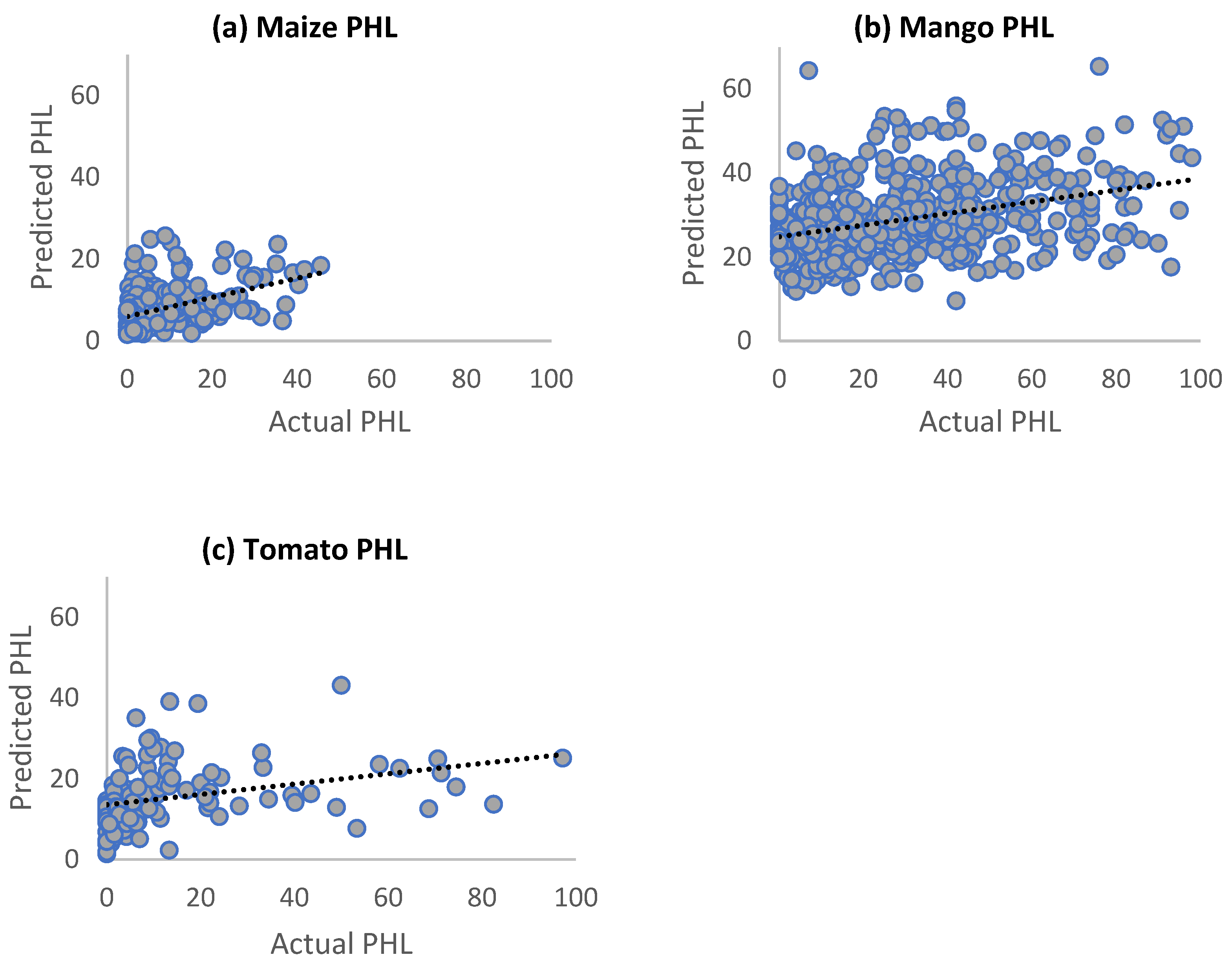
3.1. Random Forest Models

The proportion of variance explained (R-squared) was low for the predictive models of the three value chains (Table 4). The low proportion of variance explained is also reflected in the predicted vs. actual value plots of each crop chain (Figure 2).
Obtaining such low R-squared values in a Random Forest regression model is not uncommon, especially when using a large dataset with irregular patterns [25], such as the YWI dataset. The fact that the PHL values were estimated by farmers and not measured likely led to errors, which in turn contributed to the lower R-squared values, as is sometimes the case in social science studies [38]. One way to minimize the errors caused by estimating would be to measure PHL by quantifying each crop’s total weight loss and subsequently expressing it as a percentage of the total harvested weight [39]. The Random Forest model summary also produced the mean squared residual values listed in Table 4, which can be used to compare alternative predictive models to the Random Forest predictive models used in this study.

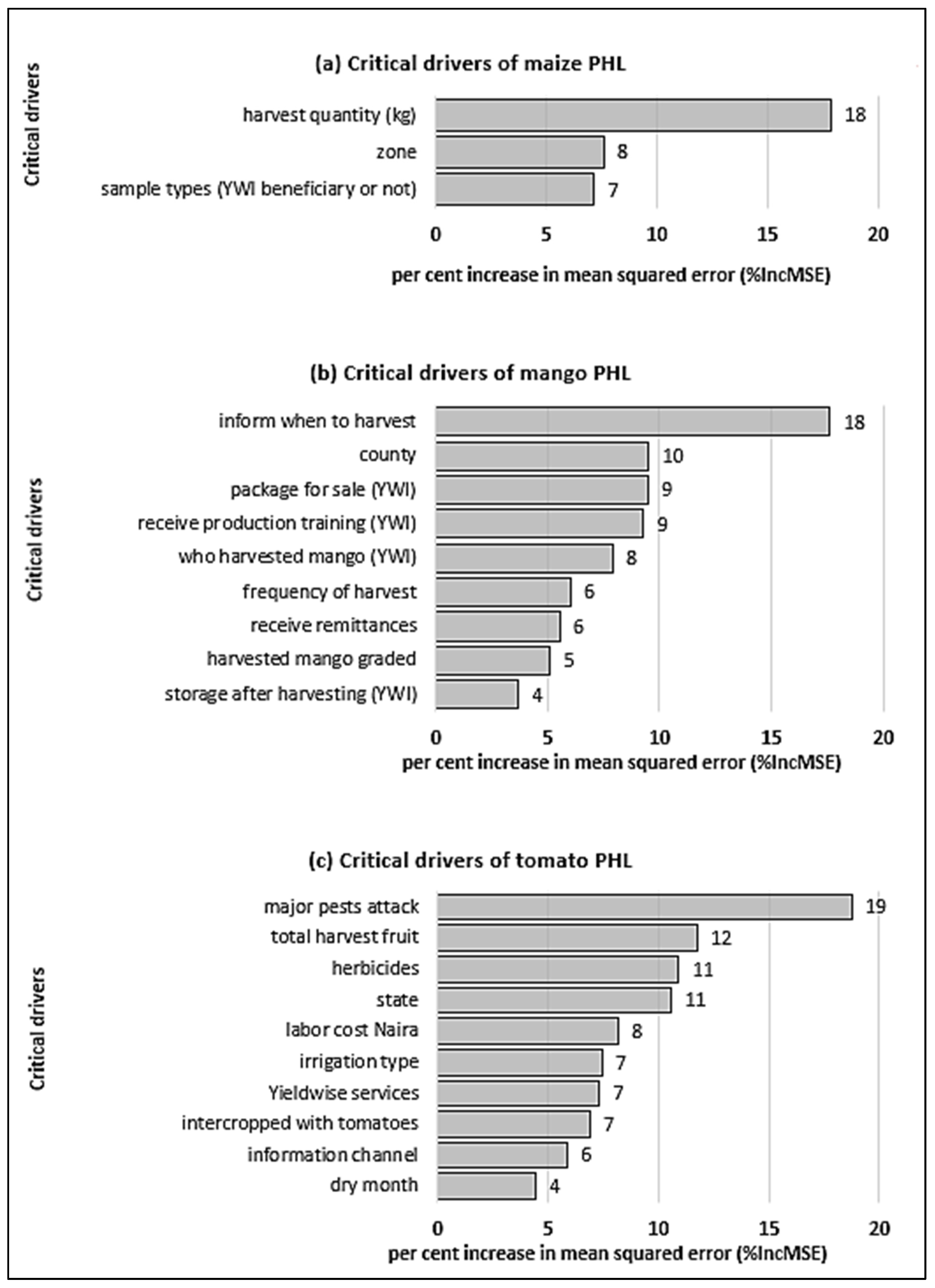
3.2. Critical Drivers of PHL

Overall, the number of critical drivers of PHL in the mango and tomato value chains shown in Figure 3b and Figure 3c, respectively, is approximately three times larger than those in the maize value chain shown in Figure 3a. Hence, these results suggest that perishable crops have more critical drivers of PHL than nonperishable crops. Kiaya [40] supports this notion, as PHL in nonperishable crops is primarily due to exogenous factors such as moisture, insects, or rodents, while PHL in perishable crops is usually due to exogenous factors and endogenous factors such as respiration, transpiration, and germination.
Additionally, the most critical drivers of PHL, labeled “the quantity (kg) of maize harvested by a smallholder farmer” (Figure 3a), “the method used to know when to begin mango harvest” (Figure 3b), and “the type of pest that attacked the tomato plant” (Figure 3c), are all related to either pre-harvest or harvest activities. Hence, these results suggest that PHL reduction efforts should start before a harvest and continue during the harvest. Incidentally, several studies have attempted to understand how pre-harvest factors affect PHL. For example, [41] looked at how physiological processes and field management strategies influenced the ultimate quality of perishable crops. Similarly, [42] established that the prevention of pre-harvest infection of maize by toxigenic A. flavus strains should be a critical control point to reduce PHL due to aflatoxin contamination.
The per cent increase in mean squared error (%IncMSE) represents the mean decrease of accuracy in predictions when a given predictor or independent variable is excluded from the predictive model. YWI refers to critical drivers related to the YieldWise Initiative.
Lastly, two types of critical drivers were ubiquitous across all three crop value chains (Figure 3). First, the geographic location of the smallholder farmer (SHF) was labeled as “zone” in the maize value chain, “province” in the mango value chain, and “state” in the tomato value chain. Second, the affiliation of a SHF with the YWI defined as the “sample types” in the maize value chain, the “type of packaging” material in the mango value chain, and the "YWI services" in the tomato value chain. These results also indicate that the YWI played an important role as a driver of PHL reduction in the three value chains [43]. While the geographic location of a SHF can be difficult to modify [44], the various YWI services could be further explored to identify combinations that best reduce PHL. For this purpose, an online dashboard was created and made accessible at https://phldashboard.shinyapps.io/phldashboard/ (accessed on 8 May 2023). Screenshots of the dashboard can be found in Appendix A.

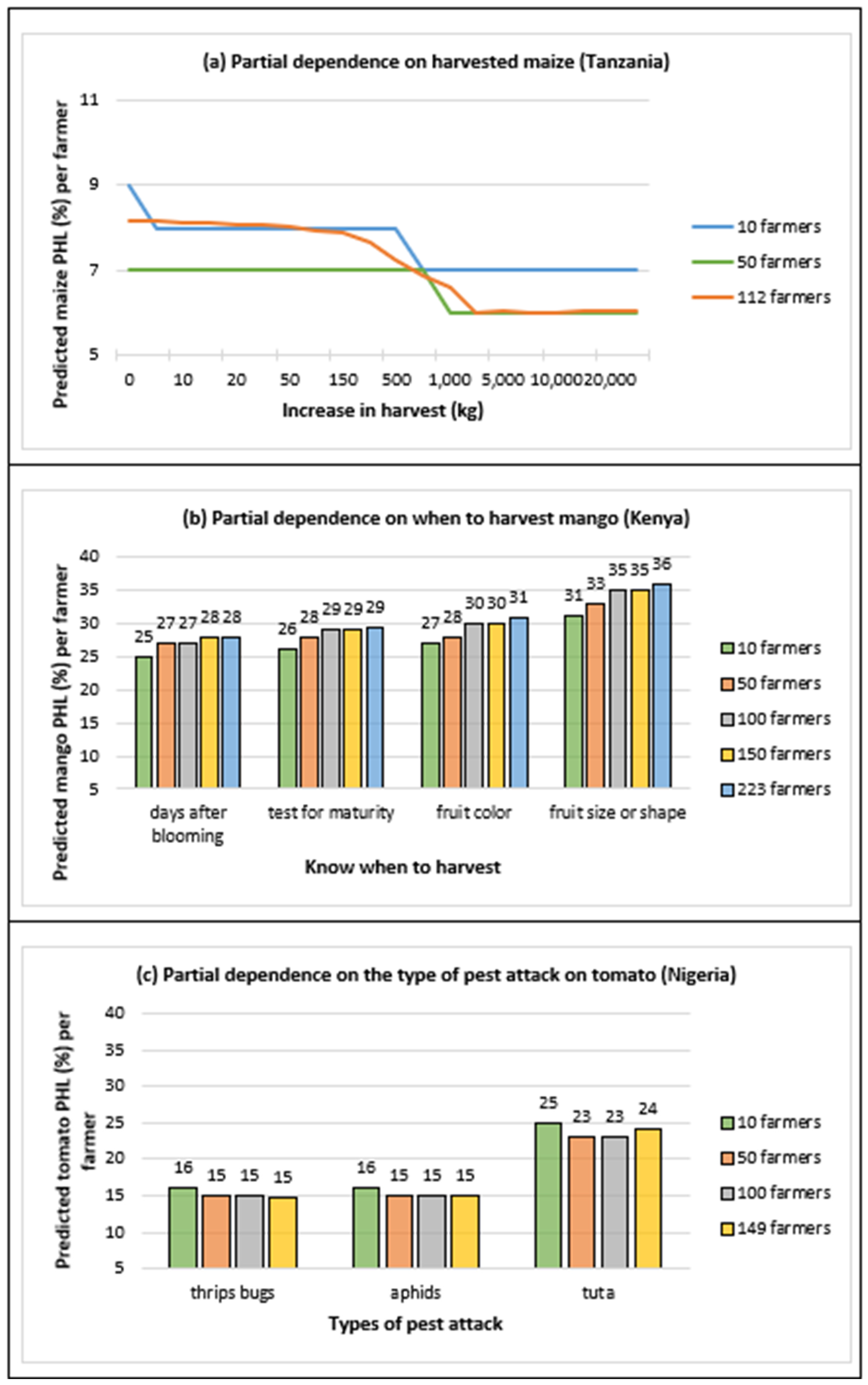
3.3. Assessing the Critical Drivers of PHL

The assessment of the critical drivers of PHL was carried out through partial dependence plots (Figure 4). These show the relationship between the most critical driver in each value chain, the PHL of each crop, and the number of SHFs. In the maize value chain, the results reveal that as the quantity of harvested maize increases, typically to more than 1000 kg, the maize PHL decreases, regardless of the change in the number of farmers.
In the mango value chain, counting the number of days after blooming to know when to begin harvest was associated with the least PHL. Incidentally, several studies have used the number of days after blooming to either determine the optimal mango harvest date to mitigate PHL during storage [45] or know when mango fruit develops the best organoleptic characteristics during ripening [46,47]. The partial dependence plot in Figure 4b also reveals that the mango PHL increases as the levels change from “days after blooming” to “fruit size or shape”. Moreover, the PHL increases monotonically as the number of farmers at each level changes from 10 to 263. However, the PHL increase due to changes in the levels (from "days after blooming" to “fruit size or shape”) is larger than the increase due to changes in the number of farmers (from 10 to 223) at each level. These results suggest that an optimum PHL mitigation practice or technology should be identified first before increasing its adoption among farmers.
In the tomato value chain, Thysanoptera, ”thrips bugs”, and Emitteri, ”aphids”, are equally associated with less PHL than the tomato leaf miner Tuta absoluta, “tuta”. Incidentally, other studies have reported the lepidoptera “tuta” as a destroyer of tomato plants in seven northern states in Nigeria, mainly due to SHFs lacking knowledge of integrated pest management practices [48,49]. Like the maize and mango value chains, as the levels of the "types of pest attack" change from Thysanoptera, “thrips bugs”, to Emitteri, “aphids”, and then to Tuta absoluta, “tuta” (Figure 4c), the shift in tomato PHL is more pronounced than when changing the number of farmers at each level.
In addition to the established relationship between the levels of various critical drivers and PHLs, it should be noted that PHL is mainly impacted by the change in the levels of a critical driver rather than the change in the number of SHFs at each level.
Since PHL is a multifaceted issue that requires considering multiple critical drivers at a time, an online dashboard was created to explore the relationship between critical drivers, the PHL of each crop, and the desired number of SHFs. The ability to insert a selected number of farmers in the dashboard allows the user to predict PHLs based on a new, arbitrary number of farmers that are not part of the YWI dataset. The online dashboard is accessible at https://phldashboard.shinyapps.io/phldashboard/ (accessed on 8 May 2023) and is described in Appendix A.

4. Conclusions

This study used Random Forest modeling to analyze the YWI data collected by the Rockefeller Foundation YieldWise Initiative in three value chains, namely maize in Tanzania, mango in Kenya, and tomato in Nigeria. The following conclusions emerged from this analysis.
  • Three critical drivers of PHL were identified in the maize value chain, nine in the mango value chain, and ten in the tomato value chain. Hence, perishable crops such as tomato and mango have more critical drivers to consider when attempting to reduce PHL than nonperishable crops such as maize.
  • The most critical drivers of PHL were the quantity of maize harvested by a smallholder farmer in the maize value chain, the method used to know when to begin mango harvest in the mango value chain, and the type of pest that attacked the tomato plant in the tomato value chain. It was then noted that the most critical drivers are all related to pre-harvest and harvest activities in the field. Hence, PHL reduction efforts should begin in the field before harvest and continue during harvest.
  • The critical drivers of PHL fall into two categories: passive critical drivers that are difficult to manipulate, such as the geographic area within which a smallholder farmer lives, and active critical drivers that are easier to manage, such as the services provided by the YieldWise Initiative. Moreover, the geographic location of a smallholder farmer and the smallholder farmers’ affiliation with the YieldWise Initiative were both ubiquitous drivers across all three value chains.
  • PHL is impacted by changes in the levels of a critical driver as well as changes in the number of smallholder farmers at each level, although the former has a much higher impact. Hence, the optimum PHL mitigation practices or technologies should be identified first before attempting to increase their adoption among smallholder farmers.
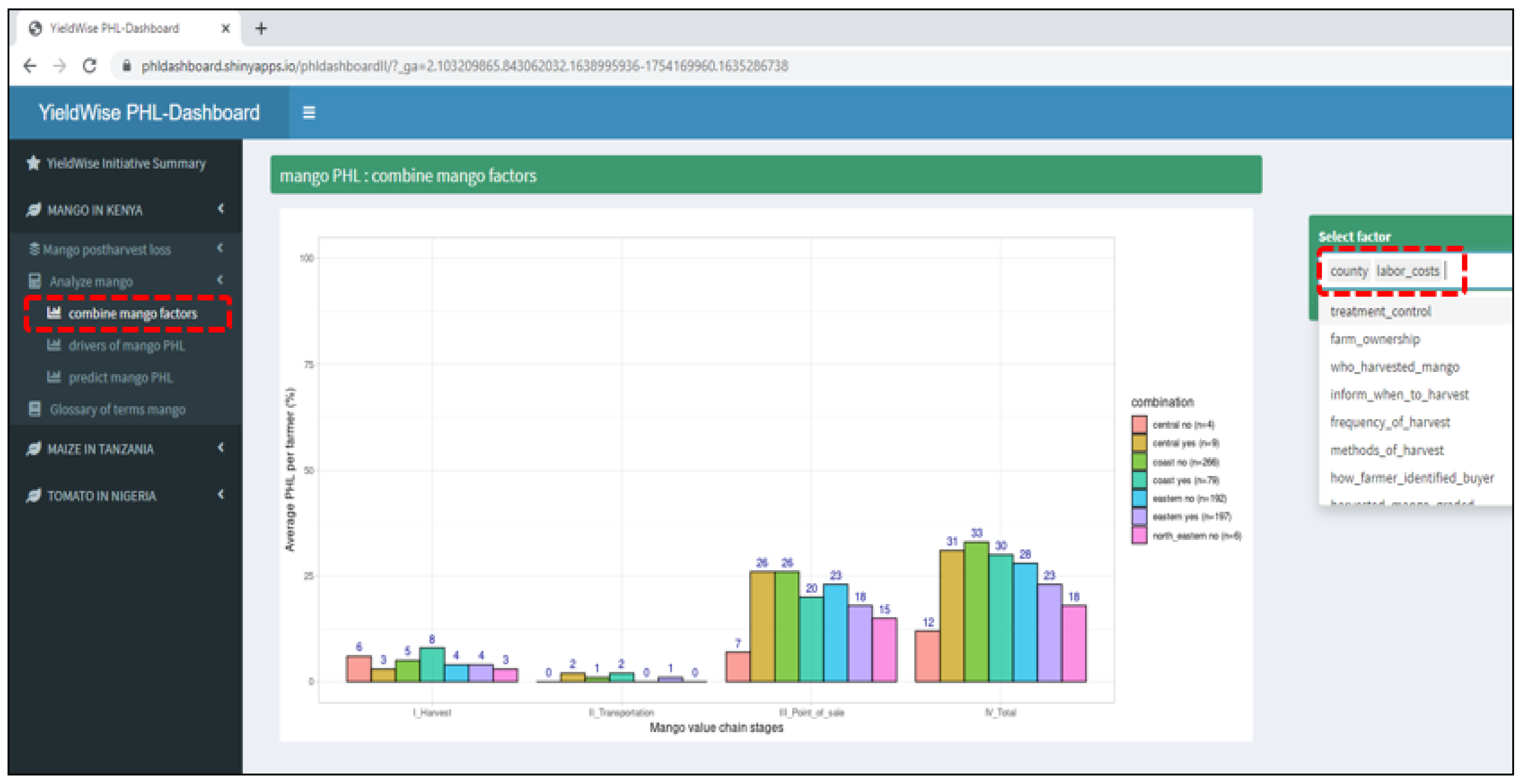
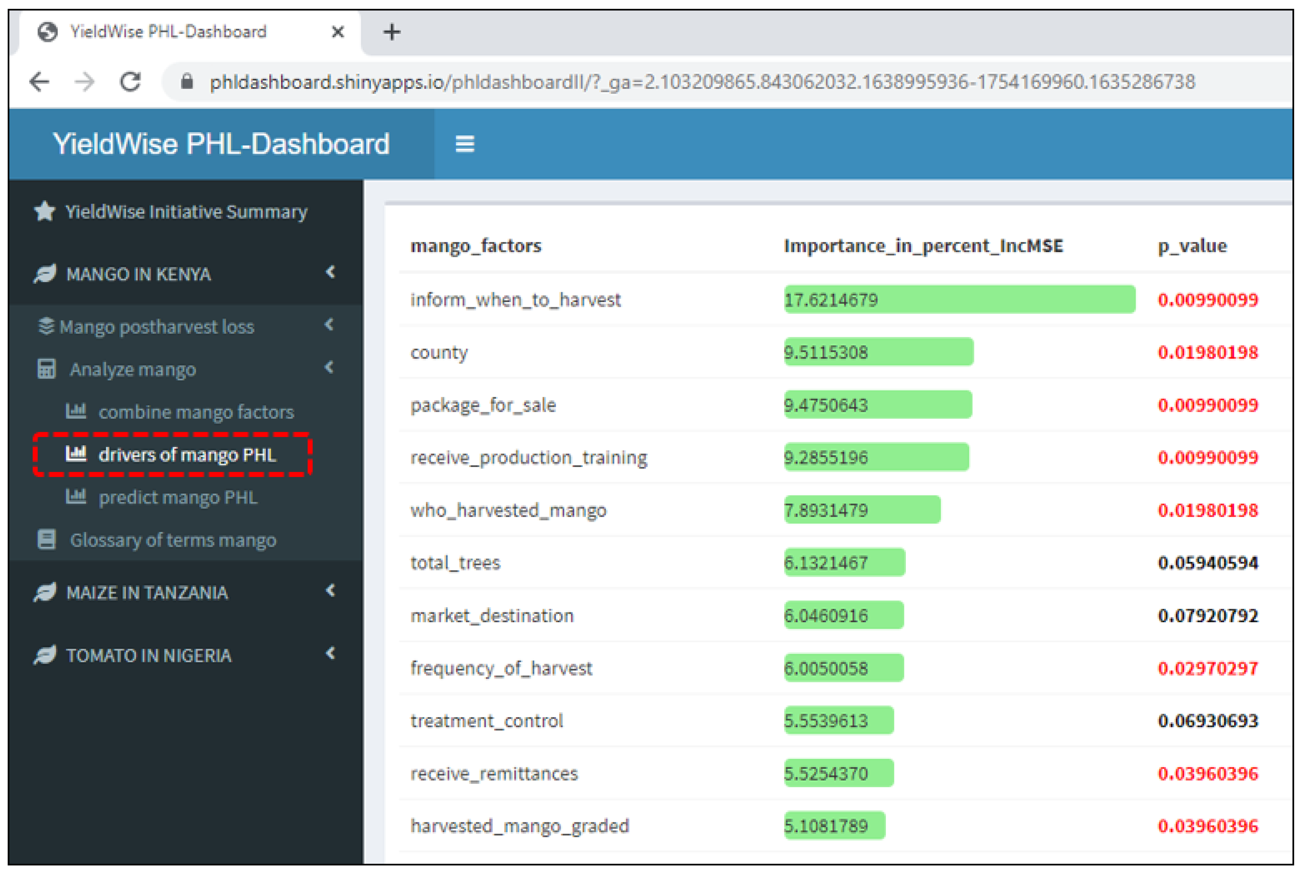
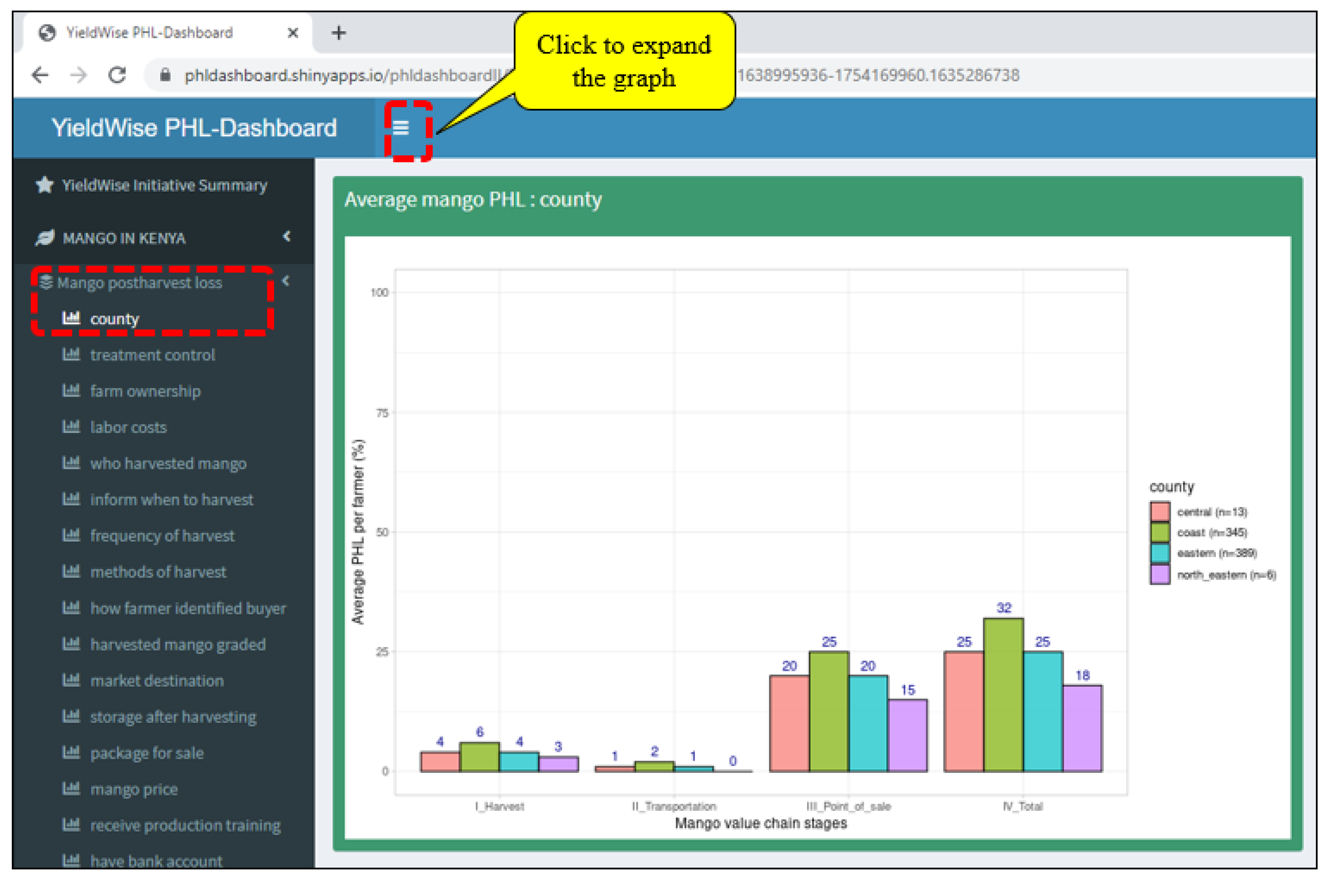
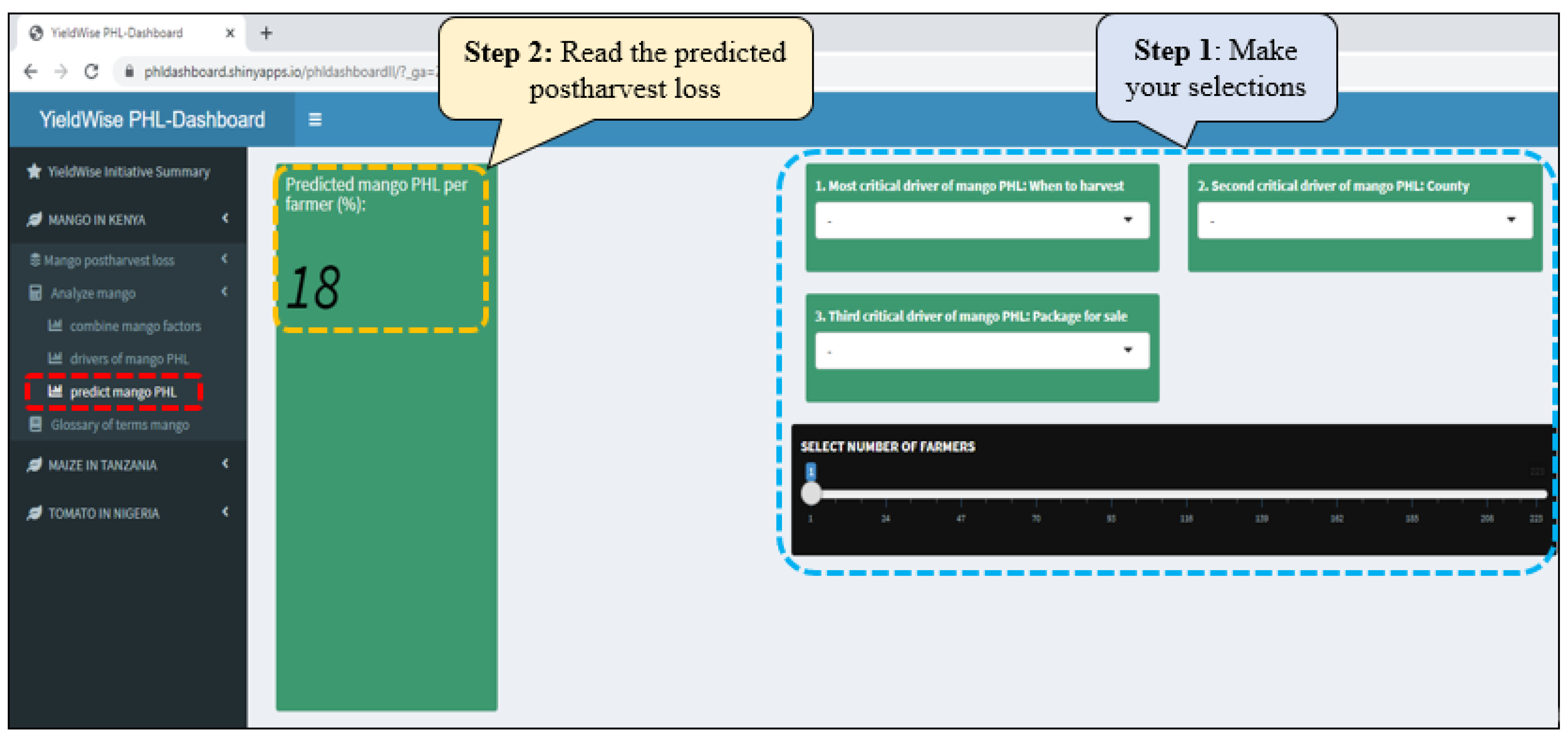
  • An online dashboard was created to (a) visually display maize, mango, and tomato PHLs in bar graphs for the numerous variables found in the YieldWise Initiative dataset, (b) rank the critical drivers of maize, mango, and tomato PHL reduction, and (c) explore the relationship between several critical drivers in each value chain, the PHL of each crop, and a desired number of smallholder farmers.
While the data that led to the above conclusions were estimated by farmers and not measured, applying the Random Forest regression algorithm to assess effects across the three different agricultural commodity types is a strength of this research.

Author Contributions

Conceptualization, H.C., D.M. and S.O.; data curation, H.C.; formal analysis, H.C. and S.O.; investigation, H.C., D.M., S.O. and S.S.; methodology, H.C., D.M. and S.O.; software, H.C. and S.O.; visualization, H.C. and D.M.; roles/writing—original draft, H.C.; writing—review and editing, H.C. and D.M.; funding acquisition, D.M. and S.S.; project administration, D.M. and S.S.; resources, D.M. and S.S.; supervision, D.M., S.O. and S.S.; validation, D.M., S.O. and S.S. All authors have read and agreed to the published version of the manuscript.

Funding

Funding for this study was provided by The Rockefeller Foundation (2018 FOD 004), the Foundation for Food and Agriculture Research (DFs-18-0000000008), and the Iowa Agriculture and Home Economics Experiment Station (DD14481).

Data Availability Statement

An online interactive mango PHL dashboard was created at https://phldashboard.shinyapps.io/phldashboard/ (accessed on 8 May 2023) to support this study’s results.

Acknowledgments

The authors would like to thank The Rockefeller Foundation, the Foundation for Food and Agriculture Research, and the Iowa Agriculture and Home Economics Experiment Station for providing funding which made this research possible.

Conflicts of Interest

The funders had no role in the design of this study, analyses, or interpretation of data, in the writing of the manuscript, or in the decision to publish the results.

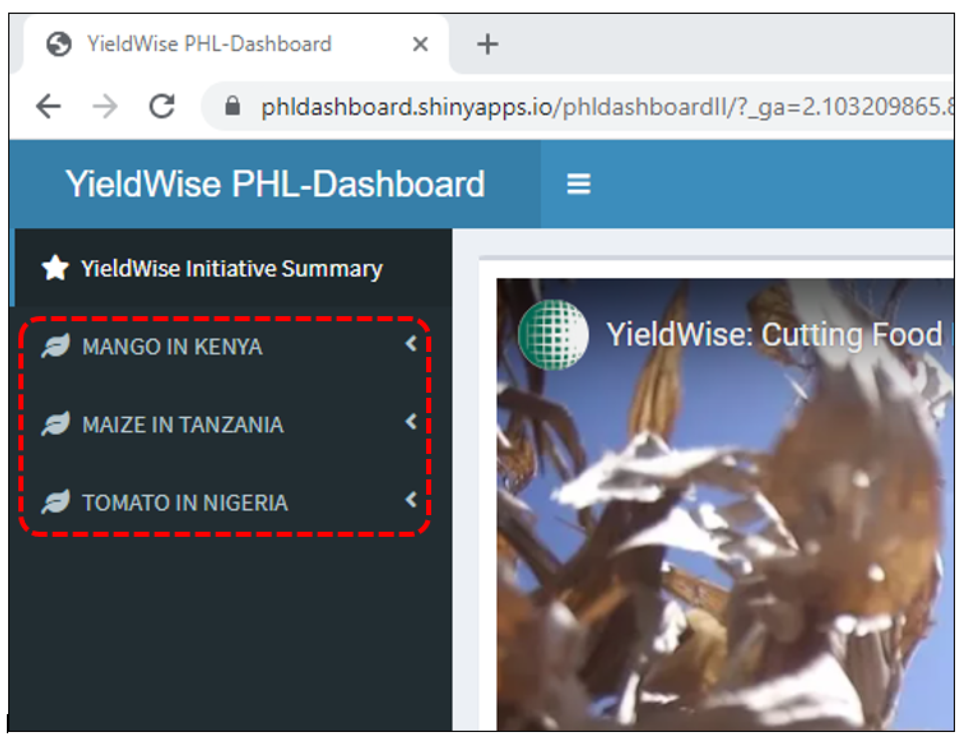
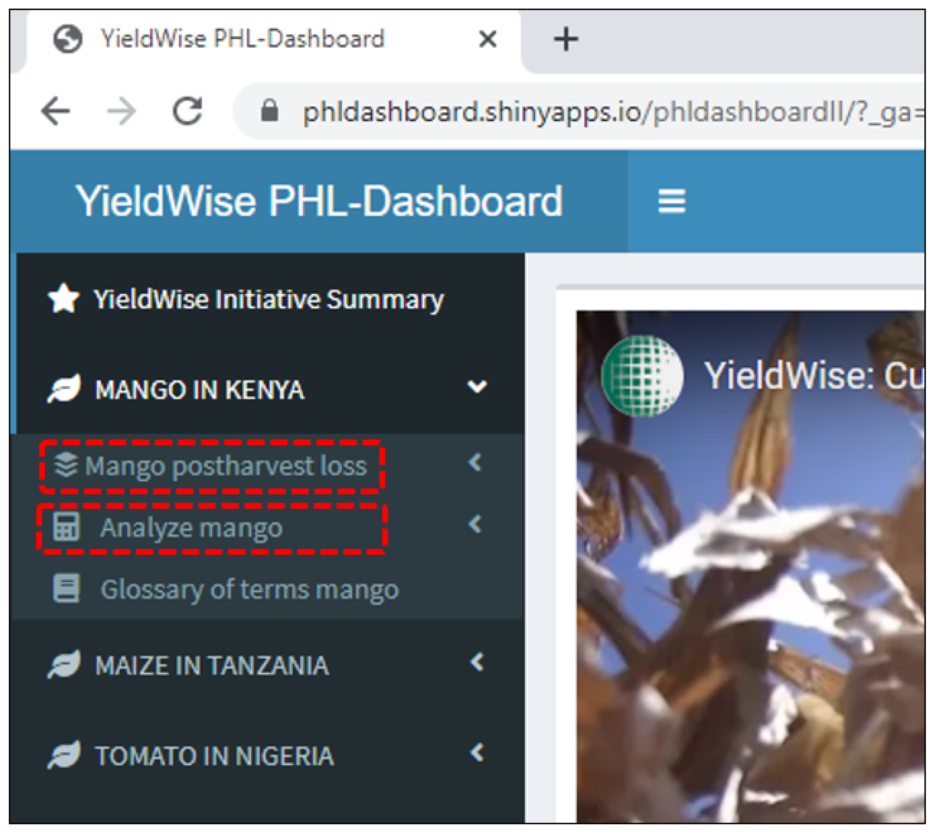
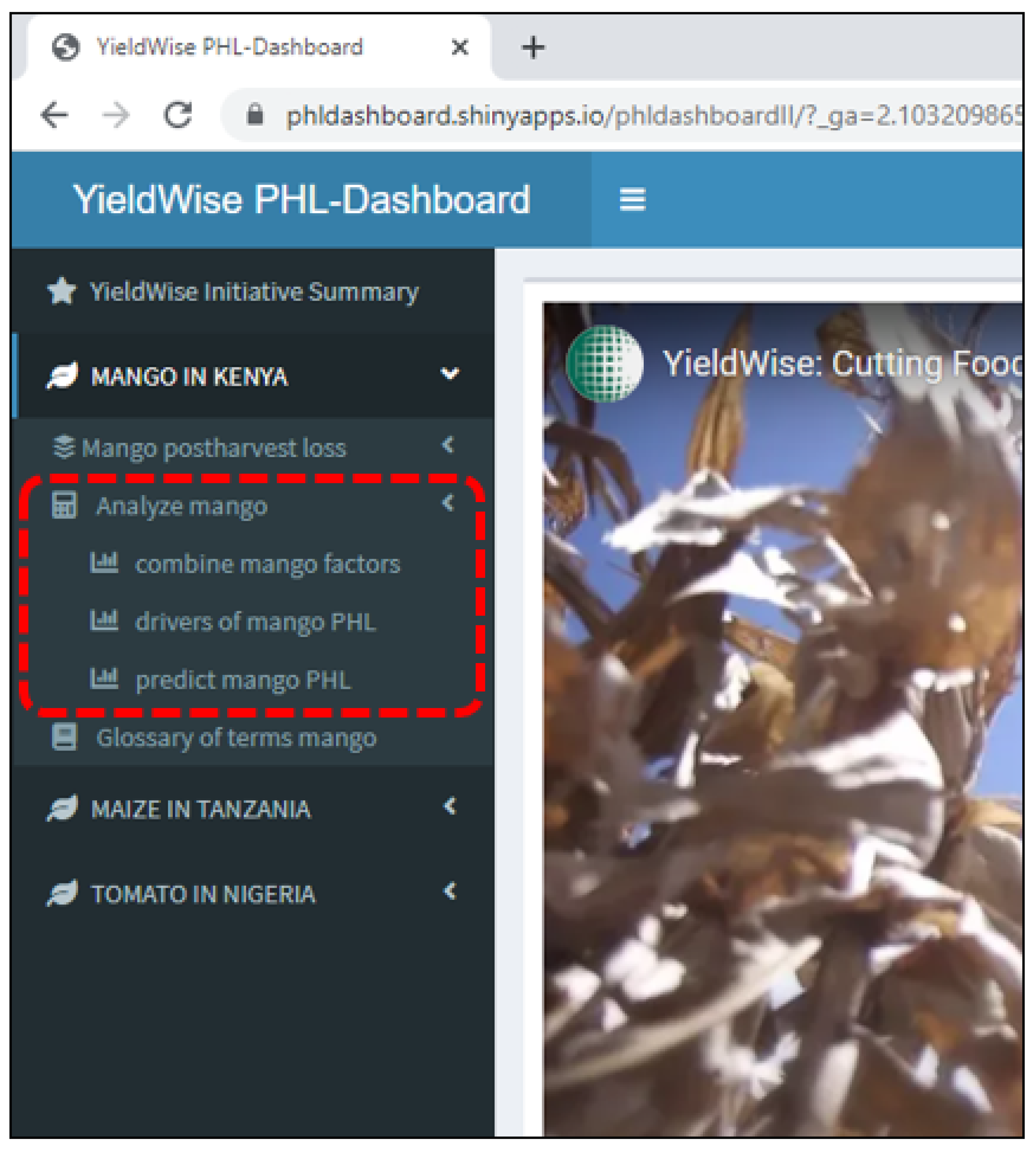
Appendix A. YieldWise Initiative PHL Data Dashboard

This online dashboard serves as a quantitative information management tool that
  • Provides a visual display of the maize, mango, and tomato postharvest losses (PHLs) in the form of bar graphs as a function of the numerous variables found in the Rockefeller YieldWise Initiative datasets.
  • Ranks the critical drivers of the maize, mango, and tomato PHLs in order of importance.
  • Predicts the maize, mango, and tomato PHLs as a function of their three most critical drivers as well as the number of smallholder farmers of interest.
The dashboard can be accessed by copying the following link into a web browser: https://phldashboard.shinyapps.io/phldashboard/ (accessed on 8 May 2023). This will open the dashboard, which can be used as explained in Figure A1, Figure A2, Figure A3, Figure A4, Figure A5, Figure A6 and Figure A7 below.
Figure A1. On the left-hand side of the screen is a menu item with the three value chains of the YieldWise Initiative.
Agriculture 13 01912 g0a1
Figure A2. The user can expand a desired value chain by clicking on it. This will allow them to either visualize PHL or analyze PHL.
Agriculture 13 01912 g0a2
Figure A3. By selecting “Mango postharvest loss” as shown in the figure above, the user will access a list of variables. The user can then select a desired variable such as the “county” variable selected in the figure above as an example. The user will then automatically see a bar graph of various PHL along the value chain, categorized by counties. The number of farmers in each category of the county is also specified in the legend. Finally, the user can collapse the list of variables by clicking on “Mango postharvest loss” one more time.
Agriculture 13 01912 g0a3
Figure A4. By clicking on “Analyze mango”, as shown in the figure above, the user can “combine factors”, which allows them to view PHL along the value chain as a function of combining multiple desired variables as opposed to looking at only one variable. Or the user could also select “drivers of mango PHL” to look at the critical drivers of mango PHL ranked in their order of importance, that is, from the most critical driver or variable to the least. Finally, under “Analyze mango”, the user can predict a PHL by selecting a given driver of PHL and a desired number of farmers.
Agriculture 13 01912 g0a4
Figure A5. The figure illustrates an example of how the “combine mango factors” is used to visualize PHL along the value chain as a function of combining the “county” AND “labor cost” variables.
Agriculture 13 01912 g0a5
Figure A6. This figure shows the ranking of the drivers of mango PHL, i.e., “mango_factors” in the first column, followed by their relative importance (expressed in percent in mean squared error) in driving PHL, and the p-values in the third column. The critical drivers are factors with p < 0.05 (red text in column 3).
Agriculture 13 01912 g0a6
Figure A7. This figure illustrates how to predict PHL. The user will first have to click on the “predict mango PHL” menu item circled in red. Then the user can select the desired subset or level of a given driver, as well as a desired number of farmers circled in blue. Lastly the user will be able to read the predicted PHL that will be displayed in the box circled in yellow based on the previously made selections.
Agriculture 13 01912 g0a7
The mango value chain was chosen as an example to illustrate how the dashboard works. The user can conduct the same operations in the maize and tomato value chains on the dashboard.

Appendix B. Variable Importance

Figure A8. The vertical axis lists all explanatory variables found in each value chain dataset. The horizontal axis shows the %IncMSE, which represents the importance of each explanatory variable. The red bars represent the critical drivers of PHL or the explanatory variables with statistically significant importance (p < 0.05).
Agriculture 13 01912 g0a8

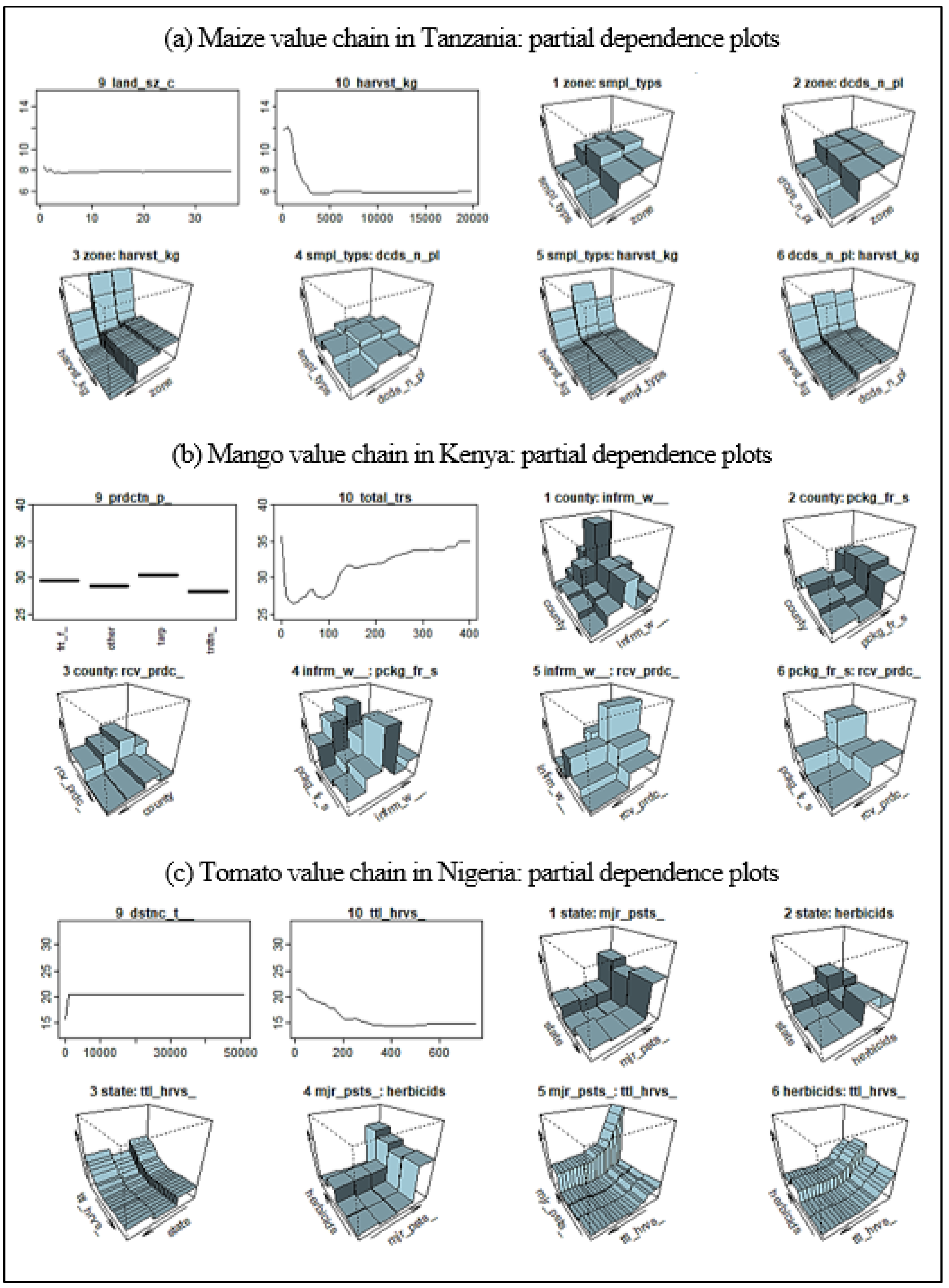
Appendix C. Partial Dependence Plots

Figure A9. Partial dependence plots (PDP). PDPs illustrate the change in the response variables for given subsets of a critical driver of the highest importance in each value chain. The response variables are averages of the predicted PHLs and are located on the vertical axis. Each exhibit shows two 2D plots of the partial dependence and four 3D plots of the combined relationships between multiple critical drivers of PHL.
Agriculture 13 01912 g0a9

References

  1. FAO. FAOSTAT. 2021. Available online: https://www.fao.org/faostat/en/#data/QCL (accessed on 24 November 2021).
  2. Flanagan, K.; Robertson, K.; Hanson, C. Reducing Food Loss Setting a Global Action Agenda; World Resources Institute: Washington, DC, USA, 2019. [Google Scholar]
  3. Owuor, T.O. Guide to Export of Fresh and Processed Mango from Kenya: A Manual for Exporters: August 2015. Available online: https://www.scribd.com/document/432862956/Mango-Export-Guide-Final (accessed on 7 April 2023).
  4. The Rockefeller Foundation. Saving Tomatoes for the Sauce. 2021. Available online: https://www.rockefellerfoundation.org/wp-content/uploads/2021/04/YieldWise-Tomato-Overview-V4.pdf (accessed on 7 April 2023).
  5. Wilson, R.T.; Lewis, J. The Maize Value Chain in Tanzania. A report from the Southern Highlands Food Systems Programme 2015. Available online: https://www.fao.org/fileadmin/user_upload/ivc/PDF/SFVC/Tanzania_maize.pdf (accessed on 7 April 2023).
  6. Mboya, R.; Tongoona, P.; Derera, J.; Mudhara, M.; Langyintuo, A. The dietary importance of maize in Katumba ward, Rungwe district, Tanzania, and its contribution to household food security. Afr. J. Agric. Res. 2011, 6, 2617–2626. [Google Scholar]
  7. Muoki, P.N.; Makokha, A.O.; Onyango, C.A.; Ojijo, N.K.O. Potential contribution of mangoes to reduction of vitamin A deficiency in Kenya. Ecol. Food Nutr. 2009, 48, 482–498. [Google Scholar] [CrossRef] [PubMed]
  8. Willcox, J.K.; Catignani, G.L.; Lazarus, S. Tomatoes and cardiovascular health. Crit. Rev. Food Sci. Nutr. 2003, 43, 1–18. [Google Scholar] [CrossRef] [PubMed]
  9. Grant, W.; Kadondi, E.; Mbaka, M.; Ochieng, S. Opportunities for Financing the Mango Value Chain: A Case Study of Lower Eastern Kenya; FSD Kenya: Nairobi, Kenya, 2015; p. 52. [Google Scholar]
  10. Wangithi, C.M.; Muriithi, B.W.; Belmin, R. Adoption and dis-adoption of sustainable agriculture: A case of farmers’ innovations and integrated fruit fly management in kenya. Agriculture 2021, 11, 338. [Google Scholar] [CrossRef]
  11. Suri, T.; Udry, C. Agricultural Technology in Africa. J. Econ. Perspect. 2022, 36, 33–56. [Google Scholar] [CrossRef]
  12. APHLIS. APHLIS+. 2021. Available online: https://www.aphlis.net/en (accessed on 4 May 2021).
  13. Engineering for Change. Landscape analysis of Post-Harvest Technologies for Mango Production in East Africa. 2020. Available online: https://www.engineeringforchange.org/wp-content/uploads/2020/10/landscape_analysis_mango_postharvest_tech.pdf (accessed on 7 April 2023).
  14. Ugonna, C.; Jolaoso, M.; Onwualu, A. Tomato Value Chain in Nigeria: Issues, Challenges and Strategies. J. Sci. Res. Rep. 2015, 7, 501–515. [Google Scholar] [CrossRef]
  15. Sheahan, M.; Barrett, C.B. Food loss and waste in Sub-Saharan Africa: A critical review. Food Policy 2017, 70, 1–12. [Google Scholar] [CrossRef]
  16. Xie, H.; Perez, N.; Anderson, W.; Ringler, C.; You, L. Can Sub-Saharan Africa feed itself? The role of irrigation development in the region’s drylands for food security. Water Int. 2018, 43, 796–814. [Google Scholar] [CrossRef]
  17. Flanagan, K.; Lipinski, B.; Goodwin, L. SDG Target 12.3 on Food Loss and Waste: 2019 Progress Report. 2019, pp. 1–16. Available online: https://champions123.org/sites/default/files/2020-09/champions-12-3-2019-progress-report.pdf (accessed on 7 April 2023).
  18. The Rockefeller Foundation. YieldWise—The Rockefeller Foundation. 2022. Available online: https://www.rockefellerfoundation.org/initiative/yieldwise/ (accessed on 8 January 2022).
  19. Chikez, H.; Maier, D.; Sonka, S. Mango postharvest technologies: An observational study of the yieldwise initiative in Kenya. Agriculture 2021, 11, 623. [Google Scholar] [CrossRef]
  20. Best, K.B.; Gilligan, J.M.; Baroud, H.; Carrico, A.R.; Donato, K.M.; Ackerly, B.A.; Mallick, B. Random forest analysis of two household surveys can identify important predictors of migration in Bangladesh. J. Comput. Soc. Sci. 2020, 4, 77–100. [Google Scholar] [CrossRef]
  21. Finlay, S. Predictive Analytics, Data Mining and Big Data; Springer: Berlin/Heidelberg, Germany, 2014. [Google Scholar] [CrossRef]
  22. Shmueli, G. To explain or to predict? Stat. Sci. 2010, 25, 289–310. [Google Scholar] [CrossRef]
  23. Kern, C.; Klausch, T.; Kreuter, F. Tree-based machine learning methods for survey research. Surv. Res. Methods 2019, 13, 73–93. [Google Scholar] [PubMed]
  24. Kuhn, M.; Johnson, K. Applied Predictive Modeling; Springer Science Business Media: New York, NY, USA, 2013. [Google Scholar] [CrossRef]
  25. Hengsdijk, H.; de Boer, W.J. Post-harvest management and post-harvest losses of cereals in Ethiopia. Food Secur. 2017, 9, 945–958. [Google Scholar] [CrossRef]
  26. Criminisi, A.; Shotton, J. Decision Forests for Computer Vision and Medical Image Analysis; Springer Science Business Media: New York, NY, USA, 2013. [Google Scholar]
  27. Breiman, L. Random Forests. Mach. Learn. 2001, 45, 5–32. [Google Scholar] [CrossRef]
  28. James, G.; Witten, D.; Hastie, T.; Tibshirani, R. An Introduction to Statistical Learning; 8th Printing 2017; Springer: New York, NY, USA, 2013; Volume 102. [Google Scholar] [CrossRef]
  29. Gholamy, A.; Kreinovich, V.; Kosheleva, O. Why 70/30 or 80/20 Relation Between Training and Testing Sets: A Pedagogical Explanation. Comput. Sci. 2018, 1–6. [Google Scholar]
  30. Kuhn, M. Building predictive models in R using the caret package. J. Stat. Softw. 2008, 28, 1–26. [Google Scholar] [CrossRef]
  31. Williams, G. Data Mining with Rattle and R: The Art of Excavating Data for Knowledge Discovery; Springer: New York, NY, USA, 2011. [Google Scholar] [CrossRef]
  32. Perner, P. Machine Learning and Data Mining in Pattern Recognition. In Proceedings of the 7th International Conference, MLDM 2011, New York, NY, USA, 30 August–3 September 2011; Volume 2961. [Google Scholar]
  33. Couronné, R.; Probst, P.; Boulesteix, A.-L. Random forest versus logistic regression: A large-scale benchmark experiment. BMC Bioinform. 2018, 19, 27. [Google Scholar] [CrossRef]
  34. Grömping, U. Variable importance assessment in regression: Linear regression versus random forest. Am. Stat. 2009, 63, 308–319. [Google Scholar] [CrossRef]
  35. Friedman, J.H. Greedy function approximation: A gradient boosting machine. Ann. Stat. 2001, 29, 1189–1232. [Google Scholar] [CrossRef]
  36. Greenwell, B.M. pdp: An R package for constructing partial dependence plots. R J. 2017, 9, 421–436. [Google Scholar] [CrossRef]
  37. Milborrow, S. Plotting Regression Surfaces with Plotmo Stephen Milborrow. 2019. Available online: http://www.milbo.org/doc/plotmo-notes.pdf (accessed on 7 April 2023).
  38. Itaoka, K. Regression and Interpretation of Low R-squared. In Proceedings of the Social Research Network 3rd Meeting, Noosa, Australia, 12–13 April 2012. [Google Scholar]
  39. Hurburgh, C.R., Jr.; Bern, C.J.; Wilcke, W.F.; Anderson, M.E. Shrinkage and Corn Quality Changes in on-Farm Handling Operations. Trans. ASAE 1983, 26, 1854–1857. [Google Scholar] [CrossRef]
  40. Kiaya, V. Post-Harvest Losses and Strategies to Reduce Them. 2014. Available online: https://www.actioncontrelafaim.org/wp-content/uploads/2018/01/technical_paper_phl__.pdf (accessed on 7 April 2023).
  41. Weston, L.A.; Barth, M.M. Preharvest factors affecting postharvest quality of vegetables. HortScience 1997, 32, 812–816. [Google Scholar] [CrossRef]
  42. Mahuku, G.; Nzioki, H.S.; Mutegi, C.; Kanampiu, F.; Narrod, C.; Makumbi, D. Pre-harvest management is a critical practice for minimizing aflatoxin contamination of maize. Food Control. 2019, 96, 219–226. [Google Scholar] [CrossRef]
  43. Sonka, S.; Lee, H.; Shah, S. The YieldWise Approach to Post-Harvest Loss Reduction: Creating Market-Driven Supply Chains to Support Sustained Technology Adoption. Agriculture 2023, 13, 910. [Google Scholar] [CrossRef]
  44. Delgado, L.; Schuster, M.; Torero, M. The Reality of Food Losses: A New Measurement Methodology; no. IFPRI Discussion Paper 01686; International Food Policy Research Institute: Washington, DC, USA, 2017; p. 40. [Google Scholar]
  45. Mathieu, L.; Jacques, J. Quality and maturation of mango fruits of cv. Cogshall in relation to harvest date and carbon supply. Aust. J. Agric. Res. 2006, 57, 419–426. [Google Scholar]
  46. Dick, E.; N’DaAdopo, A.; Camara, B.; Moudioh, E. Influence of maturity stage of mango at harvest on its ripening quality. Fruits 2009, 64, 13–18. [Google Scholar] [CrossRef]
  47. Stathers, T.; Holcroft, D.; Kitinoja, L.; Mvumi, B.M.; English, A.; Omotilewa, O.; Kocher, M.; Ault, J.; Torero, M. A scoping review of interventions for crop postharvest loss reduction in sub-Saharan Africa and South Asia. Nat. Sustain. 2020, 3, 821–835. [Google Scholar] [CrossRef]
  48. Borisade, O.A.; Kolawole, A.O.; Adebo, G.M.; Uwaidem, Y.I. The tomato leafminer (Tuta absoluta) (Lepidoptera: Gelechiidae) attack in Nigeria: Effect of climate change on over-sighted pest or agro-bioterrorism? J. Agric. Ext. Rural Dev. 2017, 9, 163–171. [Google Scholar] [CrossRef]
  49. Bala, I.; Mukhtar, M.M.; Saka, H.K.; Abdullahi, N.; Ibrahim, S.S. Determination of insecticide susceptibility of field populations of tomato leaf miner (Tuta absoluta) in northern Nigeria. Agriculture 2019, 9, 7. [Google Scholar] [CrossRef]
Figure 1. Regression Random Forest model and predictions. Web refers to the online dashboard.
Agriculture 13 01912 g001
Figure 2. Predicted PHL vs. actual PHL.
Agriculture 13 01912 g002
Figure 3. Critical drivers of PHL.
Agriculture 13 01912 g003
Figure 4. Partial dependence plots for the most critical drivers of PHL.
Agriculture 13 01912 g004
Table 1. Maize value chain data summary.
VariablesLevels (Subset)Number of Farmers or Observations (n)21. Average Land Size (ac) per Farmer22. Average Maize Harvest (kg) per Farmer per SeasonAverage Maize PHL (%) per Farmer per Season
1. genderfemale161428367
male220446267
2. zonecentral738241013
coastal242244514
southern highlands284343656
3. sample typesbeneficiary146346276
control1396321011
other96336735
4. YieldWise trainingfemale adults57235196
female youth1260007
male adults84354496
male youth2328782
other237533938
5. decides on plantingfemale adults78327599
male adults148441639
other155441485
6. decides on harvestfemale adults77328658
male adults1045400210
male youth1349403
other199441846
7. decides on proceedsfemale adults71327769
male adults103440079
male youth1349403
other206441726
8. tarp supplieragra aggregator76343999
agro equipment stores147545727
donated125350710
other146329166
9. threshing modesmanual82333889
mechanical134644727
other165336197
10. point of salefarm115315612
homestead28531998
other333439247
village market8450137
warehouse1132041
11. transport modeother374438668
sacks on animal cart4637692
sacks on bicycle1573713
sacks on wheelbarrow2229505
12. direct clientaggregators52226611
direct consumers4458844
other372438697
13. level of drynessdry25539239
humid193447810
other104438645
very dry231438298
very humid23243015
14. sun drying practicesfield before harvesting149435729
other108438185
shallow layer stand1113364
spread threshed maize120443287
ventilated crib for cob34299111
15. mc measurement methodfarmer experience1105319110
other255440007
salt test6356444
smell-based1124402
use of machines7590783
weight-based2417655
16. storage methodhome storage32442407
improved granaries3350604
on ground in house28351355
other108535766
pics hermetic bags13461157
plastic bag161436769
plastic silos1534703
traditional granaries35433939
17. received trainingno177435149
yes204441786
18. education levelcomplete college2454002
complete primary293440017
complete secondary31541265
complete university1216201
dip certificate15379818
no formal education193260012
other76258510
postgraduate1352200
some primary163188210
some secondary10455014
19. employment statusformal sector21336065
housewife35230146
informal sector316349611
not working21429046
other21439808
retired7453014
self employed232441157
temporarily employed13337179
20. transport mode Icattle cart56441029
covered trucks16443494
open trucks51468495
other197429898
sacks on head16635427
sacks on wheelbarrow102265610
tractor28448427
wheelbarrows no sacks7325867
Table 2. Mango value chain data summary.
VariablesLevels (Subset)Number of Farmers or Observations (n)20. Average Number of Mango Trees per Farmer21. Average Mango Price (KES) per FruitAverage Mango PHL (%) per Farmer per Season
1. countycentral1359525
coast34519532
eastern38971725
northeastern69718
2. treatment controlnon beneficiary28242631
YieldWise beneficiary47149627
3. farm ownershipno13533628
yes61849628
4. labor costsno46833630
yes28569725
5. who harvested mangobuyer41158627
farmer18124633
other16143727
6. inform when to harvestdays after blooming551814
fruit color16570730
fruit size or shape4922643
other52141627
test for maturity1344629
7. frequency of harvestdaily53100731
fortnightly23136629
monthly5244634
other10951528
weekly30844726
8. methods of harvestharvesting tools4957925
other16035525
traditional practices54449630
9. how farmer identified buyerbrokers40748629
farmer-based organization121691212
other8148433
own effort25338726
10. harvested mango gradedno34649530
yes40744727
11. market destinationexport10688819
local market36245629
other23934531
processing4124634
supermarket5631425
12. storage after harvestingcold store1875625
other4955629
traditional practices68645628
13. package for saleother31446631
plastic crates32050724
traditional practices11939634
14. receive production trainingno53441631
yes21960721
15. have bank accountno37435631
yes37958726
16. have mobile money accountno9529532
yes65849628
17. receive remittancesno46747628
yes28646729
18. taken loan for farmno69544629
yes5871825
19. production PHL practicesfruit fly traps12576625
other20353827
tarp11517533
traditional practices31041629
Table 3. Tomato value chain data summary.
VariablesLevels (Subset)Number of Farmers or Observations (n)21. Average Income (NGN) per Farmer22. Average Labor Cost (NGN) per Season23. Average Frequency of Pesticide Applications per Season24. Average Distance (km) to Market25. Average Harvest (kg) per Farmer per SeasonAverage Tomato PHL (%) per Farmer per Season
1. treatment or controlcontrol166235,63046,79671821420
intervention337271,73846,15161925315
2. statejigawa134309,03843,33062118522
kano248195,53534,45252026613
katsina121337,07774,13791224719
3. genderfemale5316,20011,0006428014
male498259,25546,71961823917
4. dry monthjanuary43244,11842,53172026017
february6641,667110,000641885
august6185,00057,583676614
september52398,32770,13381921926
october229215,82337,57472125618
november106289,77863,21851521415
december61235,73725,1495152497
5. tomato varietieschibli20235,88036,0195131264
other236275,18859,66871723315
roma65296,26125,21852122917
uc82b182229,51237,80161926520
6. intercropped with tomatoesno343265,50950,78372025016
yes160247,62836,89061521719
7. main fertilizersnpk63158,84729,17751119624
other402284,89152,01871823915
ssp21144,647926653940415
urea17183,47622,17653120817
8. major pests attacksaphids50278,47235,7525715410
other287279,68554,28171623614
thrips bugs18203,92221,406592286
tuta148221,79937,63062727826
9. pesticides usagecombine329254,83653,24871825217
other12152,59262,1671422210
single162277,88731,21262121716
10. diseases attackleaf blight41177,81529,81041123810
leaf virus92180,82826,66763232618
nematodes43382,61662,74461421618
other327276,18151,82771621917
11. herbicidesglyphosate77193,07533,19763224015
manual337300,75654,20561423315
other67166,03626,79561929120
primextra22152,00431,927122918927
12. irrigation typedrip104226,74636,03962625017
flood265284,82146,74471523618
other109266,51361,07552025812
sprinkler25103,24021,1408815818
13. harvesting containersother9307,44449,88941822313
plastic crates1850023,000611702
raffia baskets474244,29645,79861924617
sacks19637,81660,0315109811
14. harvest destinationagg center9243,88952,333789934
buyer picks up164264,12854,76472929617
market197216,16830,18461120217
other133320,24759,56771623514
15. transportation method1-ton truck198273,30839,96661625415
2-ton truck48267,11551,28191724525
30-ton truck2850,00025,0001023740023
5-ton truck1115,00040,00014102344
motorcycle134225,80235,32051016817
other81276,92978,41873834514
tricycle39237,17445,42061018219
16. YieldWise servicescredit23143,97822,03945232415
inputs19238,47455,23763323925
market access73151,98537,60751023415
none177326,96863,82471820817
other186254,78733,54261725915
training25259,56259,34061126724
17. information channelfriend15234,55726,27372524027
market5239,20045,00011628030
neighbor396,66720,1676119714
other331287,46854,45471924917
phone3186,00033,33343522727
posters150,0005000325033
radio145206,38431,11851722013
18. farmer group memberno180283,34847,79251420816
yes323246,71045,56772125817
19. inputs on creditno473262,04046,14961823916
yes30224,83349,75381624824
20. contract with Dangotedo not know18136,54439,61741021417
no451267,16640,40861923617
yes34227,653128,9299153017
Table 4. Summary of the Random Forest predictive model for each value chain.
Random Forest Predictive Model Value Chainp-Value% Var Explained (R-Squared)Mean Squared Residual
Maize0.001 *2067
Mango0.001 *13447
Tomato0.001 *21327
* Indicates that the model is significant at p < 0.05.
Disclaimer/Publisher’s Note: The statements, opinions and data contained in all publications are solely those of the individual author(s) and contributor(s) and not of MDPI and/or the editor(s). MDPI and/or the editor(s) disclaim responsibility for any injury to people or property resulting from any ideas, methods, instructions or products referred to in the content.

