Article

SpikoPoniC: A Low-Cost Spiking Neuromorphic Computer for Smart Aquaponics

1
State Key Lab of Analog and Mixed Signal VLSI (AMSV), University of Macau, Macau 999078, China
2
Department of Electrical and Computer Engineering, Faculty of Science and Technology, University of Macau, Macau 999078, China
3
Department of Computer Science, Beijing Jiaotong University, Weihai 264003, China
4
Lingyange Semiconductor Inc., Zhuhai 519031, China
5
ZUMRI-LYG Joint Lab, Zhuhai UM Science and Technology Research Institute, Zhuhai 519031, China
6
School of Computing, Faculty of Engineering and Physical Sciences, University of Leeds, Leeds LS2 9JT, UK
*
Author to whom correspondence should be addressed.
Agriculture 2023, 13(11), 2057; https://doi.org/10.3390/agriculture13112057
Submission received: 5 September 2023 / Revised: 8 October 2023 / Accepted: 10 October 2023 / Published: 27 October 2023
(This article belongs to the Special Issue Digital Innovations in Agriculture—Series II)

Abstract

:
Aquaponics is an emerging area of agricultural sciences that combines aquaculture and hydroponics in a symbiotic way to enhance crop production. A stable smart aquaponic system requires estimating the fish size in real time. Though deep learning has shown promise in the context of smart aquaponics, most smart systems are extremely slow and costly and cannot be deployed on a large scale. Therefore, we design and present a novel neuromorphic computer that uses spiking neural networks (SNNs) for estimating not only the length but also the weight of the fish. To train the SNN, we present a novel hybrid scheme in which some of the neural layers are trained using direct SNN backpropagation, while others are trained using standard backpropagation. By doing this, a blend of high hardware efficiency and accuracy can be achieved. The proposed computer SpikoPoniC can classify more than 84 million fish samples in a second, achieving a speedup of at least 3369× over traditional general-purpose computers. The SpikoPoniC consumes less than 1100 slice registers on Virtex 6 and is much cheaper than most SNN-based hardware systems. To the best of our knowledge, this is the first SNN-based neuromorphic system that performs smart real-time aquaponic monitoring.

1. Introduction

The world is witnessing a rapid increase in population and a decrease in the amount of available food. The food sources are depleting faster than ever before. This is why it is crucial to develop advanced agricultural techniques. Aquaponics is a recently developed agricultural technique that combines aquaculture and hydroponics in a symbiotic way to increase the overall food production and quality. In an aquaponic system, fish excrete their waste, which is transformed into nutrients by nitrifying bacteria, which in turn are readily absorbed by plants. This symbiotic relationship is shown in Figure 1 and Figure 2. Smart aquaponic systems (SASs) first take input from sensors that collect data about the environment and then use that information for making critical decisions such as controlling the level of oxygen and nutrients in the ecosystem. The parameters may include temperature, pH level, and oxygen level. In Figure 2, the symbol N represents the number of input features, and p is a symbol for the pth hidden neuron.
Aquaponics is safer for environment than the traditional farming techniques because it limits the use of harmful chemicals [2]. The use of aquaponics can greatly resolve the water scarcity crisis as the water consumed by aquaponic systems is only 2–10% of what is used by the traditional agricultural systems. Aquaponics also plays a good role in promoting promote soil-less culture [2,3]. Despite all these advantages, only 31% of the aquaponic solutions have been found to be commercially viable due to poor management and inexperienced handlers [2]. This is where the role of deep learning (DL) comes into play. Deep learning is a proven tool to monitor and control nutrients in an aquaponic system. DL can help in the early prediction of fish size and water quality, which can in turn help in the automatic adjustment and upgradation of system parameters. For example, if a fish is smaller than the expected size, it can be provided with more food and healthy nutrition. In this context, various deep learning models have been proposed to predict water quality parameters, fish classification, fish size estimation, feeding decisions, etc. [2,4,5,6,7].
Since large-scale aquaponic systems have to deal with a huge number of parameters and require extensive monitoring, it is quite hard for humans to do all the manual work. The problem becomes more severe when there is a shortage of experienced manpower. In order to resolve these issues, automation techniques and artificial-intelligence-based systems can be extremely helpful. Such techniques and systems reduce the need for huge manpower and allow for better management at a commercial scale. Smart Systems (SSs), in the context of aquaponic systems, refer to small but intelligent electronic devices capable of performing a huge number of complex operations such as sensing, monitoring, and control in a minimal amount of time [2].
Although the literature is filled with works describing the development of smart DL systems for aquaponics, no intelligent DL system is based on dedicated hardware (HW). Here, the term dedicated hardware refers to field programmable gate arrays (FPGAs) and application-specific integrated circuits (ASICs). All the systems are implemented using microcontrollers (uCs) and/or general-purpose computers (GPCs) that are inherently slow. This is because uCs and GPCs follow a sequential model of execution. As a result, a high degree of parallelization in such systems is almost impossible. Even if there is a certain degree of parallelization in any such system, it can never match the level of parallelization offered by dedicated HW systems. Due to their slow speed, the use of uCs and GPCs in large-scale commercial aquaponic systems—where millions of parameters have to be handled in real time—can become quite problematic. There is another problem associated with the use of GPCs: they have a large area and require expensive software tools for proper operation. This certainly increases their cost and footprint and limits their usage in practical systems. FPGAs and ASICs, on the other hand, have smaller footprints, offer a higher speed, and have lower power requirements. This has been demonstrated even in this article: the use of the FPGA-based DL system is about 3369 times faster than traditional general-purpose computers. Figure 3 shows the relationship between various computing platforms in terms of efficiency and flexibility. As can be seen in Figure 3, ASICs and FPGAs are quite difficult to develop but have higher efficiency, i.e., lower power consumption, higher speed, and smaller area. Dedicated HW systems have a huge number of parallel computational elements, which makes them suitable for high speed applications. This is the basic advantage of using neuromorphic systems/accelerators (NMSs/NMAs). NMAs are accelerators that use dedicated hardware devices (FPGAs/ASICs) to implement neural networks. By doing so, a lot of improvement in system speed, energy consumption, and area can be obtained [8,9]. Section 1.2 discusses various modern neuromorphic accelerators.
There are some other shortcomings as well in the currently available works. One such shortcoming is that all these works (aquaponic systems) use artificial neural networks (ANNs) that are quite expensive and compute-intensive, especially when implemented on dedicated hardware devices such as ASICs. Though ANNs have exhibited excellent performance in the context of both classification and regression, they consume a lot of system energy and are extremely complex [10]. Spiking neural networks (SNNs), on the other hand, are more efficient than ANNs when it comes to hardware efficiency [8] since SNNs are event driven and consume lesser energy than ANNs. The primary difference between an ANN and an SNN is that the former uses continuous analog values, while the latter uses spikes for neuronal communication. These spikes are emitted by a neuron only when an important event takes place, otherwise nothing is emitted and the subsequent units remain silent [8]. This behavior is similar to the biological neurons [11,12]. In fact, the asynchronous behavior of biological neurons is the reason why the brain consumes only a few watts of energy despite having a very small area [11]. Therefore, SNNs are more bioplausible than ANNs [12,13]. In fact, since SNNs use simple spikes, they might have a very small hardware footprint, as in [9,14]. Moreover, SNNs can achieve almost the same level of accuracy as ANNs, as can be seen in [14,15,16]. This is why it is the need of the hour to develop SNN-based aquaponic systems. Another big problem in most modern studies is the lack of available data. Most datasets have a few hundred samples for system evaluation, which is insufficient to obtain reliable results. For example, the work in [3] uses only 211 samples for performance evaluation. SNN training is also a very serious issue since spikes are non-differentiable and backpropagation is not easy to apply [15,17]. Moreover, ANN-SNN conversion requires a lot of costly operations such as weight-threshold balancing [18].
Keeping all these issues in mind, we propose a novel, high-speed and small-footprint smart aquaponic system based on a spiking neural network for fish size estimation. The system can monitor and predict the size of fishes in real time. The system can classify a given input sample into one of the eight classes defined with respect to weight or length. The system can estimate both the expected length and weight of fishes based on input data. The throughput of the system is 84.23 million samples per second, i.e., the system can classify 84.23 million samples in a second. Moreover, the proposed SNN system consumes 45% fewer hardware resources than its ANN counterpart for the same level of accuracy. In fact, the proposed system is 2×–3× cheaper than most contemporary systems.
  • Main Contributions
This paper presents a novel, hardware-efficient, SNN-based neuromorphic engine for fish size estimation, which finds application in aquaponic monitoring. The system has been modeled in Verilog language at the register-transfer level (RTL). The main contributions of this work are mentioned below. A summary of these contributions is given in Figure 4.
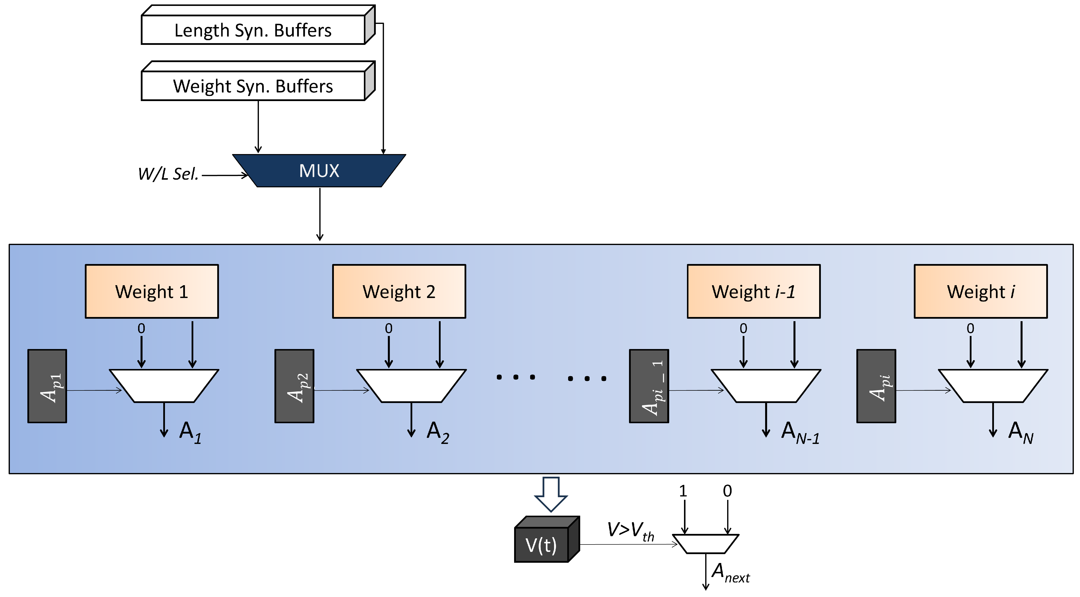
  • To provide a complete methodology to develop an aquaponic monitoring system that uses spiking neural networks to predict fish size. The system is capable of predicting both the length and weight of a fish, unlike other systems that can predict either length or weight, not both. In the proposed system, this is done using two switching buffers: one for predicting the weight, and the other one for predicting length.
  • A proposal of a novel hybrid training scheme that uses both ANN and SNN layers to achieve a blend of high accuracy and hardware efficiency. The system uses direct training for SNNs and standard backpropagation for ANN layers. The proposed implementation is much more hardware-efficient not only than a typical, fully ANN implementation but other SNN implementations too, without any loss of accuracy. The system can estimate the range of length with more than 98.03% accuracy, and the range of weight with 99.67% accuracy.
  • The system does not use any complex weight-threshold balancing mechanism, unlike various SNN training schemes [18,19], since it uses direct SNN backpropagation.
  • An SNN-based neuromorphic system implemented on a field programmable gate array (FPGA) for real-time aquaponic monitoring. It is an edge computer capable of predicting fish size (length and weight) on the basis of input parameters. The proposed edge computer can predict 8 different fish size categories based on the given data. The system can operate in the ‘fully parallel’ mode and can estimate 84.23 million samples in a second. The throughput is about 3369 times higher than a typical CPU-based software system, making it suitable for large-scale commercial use. While other systems use only a few hundred samples for testing purposes, the proposed system has been trained/tested on 175,000 samples, which proves that the obtained results are more reliable than others’.
  • The proposal of a hardware-efficient surrogate gradient that is as efficient as sigmoid but has higher flexibility. The mean-squared error between the sigmoidal derivative and the proposed derivative is 0.013%. The learning technique is suitable for developing on-chip learning (OCL) systems since the proposed surrogate gradient requires far fewer hardware resources than most gradients proposed in the literature while being extremely accurate.
The rest of this paper is organized as follows. The coming parts of this section present a review of various modern smart aquaponic systems and neuromorphic accelerators. It also presents the problem definition. Section 2 presents the training methodology for fish size estimation. Section 2 also presents the operation and details of SpikoPoniC, the proposed neuromorphic computer. The results are presented in Section 3. Finally, Section 4 concludes the work.
  • Related Work and Problem Definition
Smart aquaponic systems (SASs) are generally built using GPCs and microcontrollers (MCs) [2]. We could not find any SAS built using FPGAs/ASICs in the literature. This is where the problem lies. Modern SASs are quite complex, and MCs or GPCs are not fast enough to operate at the required speed [20,21]. Moreover, MCs and GPCs consume a lot of power and can be extremely expensive when manufactured in bulk quantities. Therefore, we chose to implement the proposed design on an FPGA. The same design can be implemented on an ASIC as well, and higher hardware efficiency can be achieved. Furthermore, we focus not only on the algorithm but also on the hardware design. This approach has been proven to be extremely effective at developing high-performance systems [9,22] since hardware efficiency is directly related to algorithmic efficiency.
Since the proposed scheme SpikoPoniC deals with both algorithm and architecture, we divide this section into two major parts. The first part presents a comprehensive review of modern smart aquaponic systems, and the second part deals with the neuromorphic accelerators. Based on the literature review, we conclude that SNNs have not yet been used for building SASs. In fact, none of the NM accelerators have been designed specifically for aquaponics.

1.1. Smart Aquaponics: Algorithms and Monitoring Systems

In the context of smart aquaponics, deep learning finds its applications, among others, in the following areas: fish size estimation, water quality prediction, plant disease diagnosis, and intelligent feeding decisions. The estimation of fish length and weight is important in order to properly manage aquaponic systems and to model stock trends. The dynamics of fish length distribution represent a key input for understanding the fish population dynamics and taking informed management decisions on exploited stocks. Nevertheless, in most fisheries the length of landed fish is still made by hand. As a result, length estimation is precise at a fish level, but due to the inherent high costs of manual sampling, the sample size tends to be small.
In [4], the authors present a scheme for fish length estimation using convolutional neural networks (CNNs). Their scheme is 93% accurate. A comparison between various popular CNN topologies for estimating the mass of Pintado Real fingerlings is given in [23]. The estimation of fish length using videos can also be very useful for developing a stable SAS. In this context, the authors in [5] present a method for underwater fish detection using videos. The system uses a ResNet-50 CNN and is 95.47% accurate. To operate a stable SAS, the early diagnosis of fish diseases can also be very helpful. In case a fish is found to be unhealthy, it can be removed from the pond; otherwise, the whole ecosystem can get disturbed. The researchers in [6] propose a scheme that can differentiate red spots on a fish from the white ones with 94.44% accuracy. Deep learning can be used to predict and control various nutrients and chemicals (moving in and out of the system) as well. For example, the authors in [24] present a scheme that can predict the concentration of oxygen in SASs. If a system contains less than the optimal level of oxygen, it can be supplied with more oxygen. Neural networks can be used to monitor other SAS parameters also, such as pH level, ammonia level, and temperature. They can also be used to make appropriate feeding decisions for plants and/or fishes [7].
Let us now discuss spiking neural networks. SNNs are the next-generation NNs whose potential has been demonstrated for a variety of applications, such as low-power image classification [8]. However, there are some major problems facing SNNs, especially in the context of SAS design.
  • Firstly, no SAS-specific SNN system is available in the literature. All the smart aquaponic systems presented in the literature use artificial neural networks for parameter prediction and other tasks.
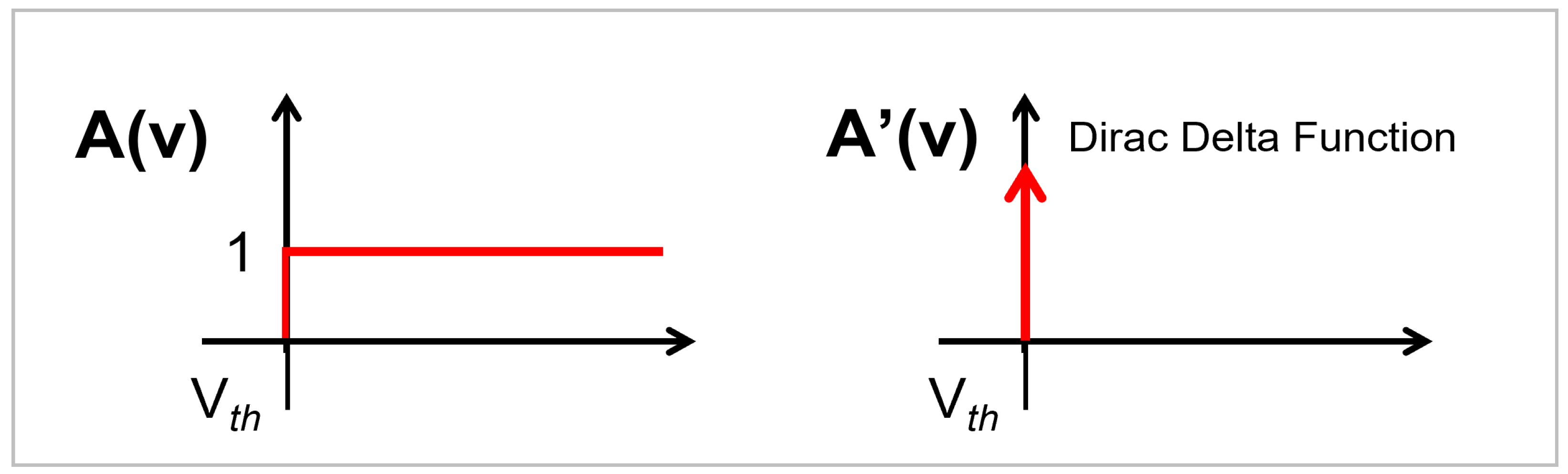
  • Secondly, most SNN systems presented in the literature yield very low accuracy, even for digit classification tasks. Only a few SNN schemes achieve high accuracy. This is because spikes are non-differentiable in nature and direct backpropagation is quite tricky to apply [15]. The non-differentiable nature of spikes is shown in Figure 5. Therefore, most researchers typically use an unsupervised algorithm spike-timing-dependent plasticity (STDP) for SNN training.
  • Many backpropagation-based SNN training schemes [16,18,19] use complex mechanisms such as weight-threshold balancing.
  • SNNs, unlike ANNs, require multiple time steps to process an input. This is why SNNs, sometimes, can consume a lot of time and hardware energy.
For example, the SNN scheme in [25] achieves 95% accuracy on MNIST dataset, even with more than five million synapses and hundreds of time steps. This is why it is crucial to develop SNN learning schemes that can yield high accuracy with a minimal network size. For instance, the work in [17] uses SNN backpropagation to achieve 98.7% accuracy with only 268,800 synapses and 8 time steps. The work in [17] is one of the rare works that do not require a long time to train SNNs. The other example is the work in [9] that requires only 10 time steps and a little over 150k synapses to reach 97.5% on MNIST. Most works, especially the ones based on STDP, require hundreds of time steps and millions of synapses to achieve reasonable accuracy, even on MNIST. The work in [26] is a good example of this. The scheme requires 700 time steps to achieve 92.63% accuracy, which is extremely low. Even backpropagation can be difficult to apply on SNNs. A good example is [27], where a 38-layer network with a complex batch form of normalization is applied to train the SNN. Though the network achieves good accuracy—equal to 92.8%—on CIFAR-10, the scheme is extremely complex to apply. Other such examples can be seen in [28,29,30].
The system in [31] achieves only 97.20% accuracy on MNIST in 1200 epochs, where each epoch contains tens of time steps. The scheme in [32] requires multiple time steps and 100 s of iterations to achieve 98.6% accuracy. To do this, multiple convolutional layers are followed by spiking layers equipped with backpropagation and STDP to achieve better accuracy. Though the scheme achieves good accuracy, the overall system is extremely complex and unsuitable for hardware implementations. Moreover, the scheme has not been tested on any aquaponics data.

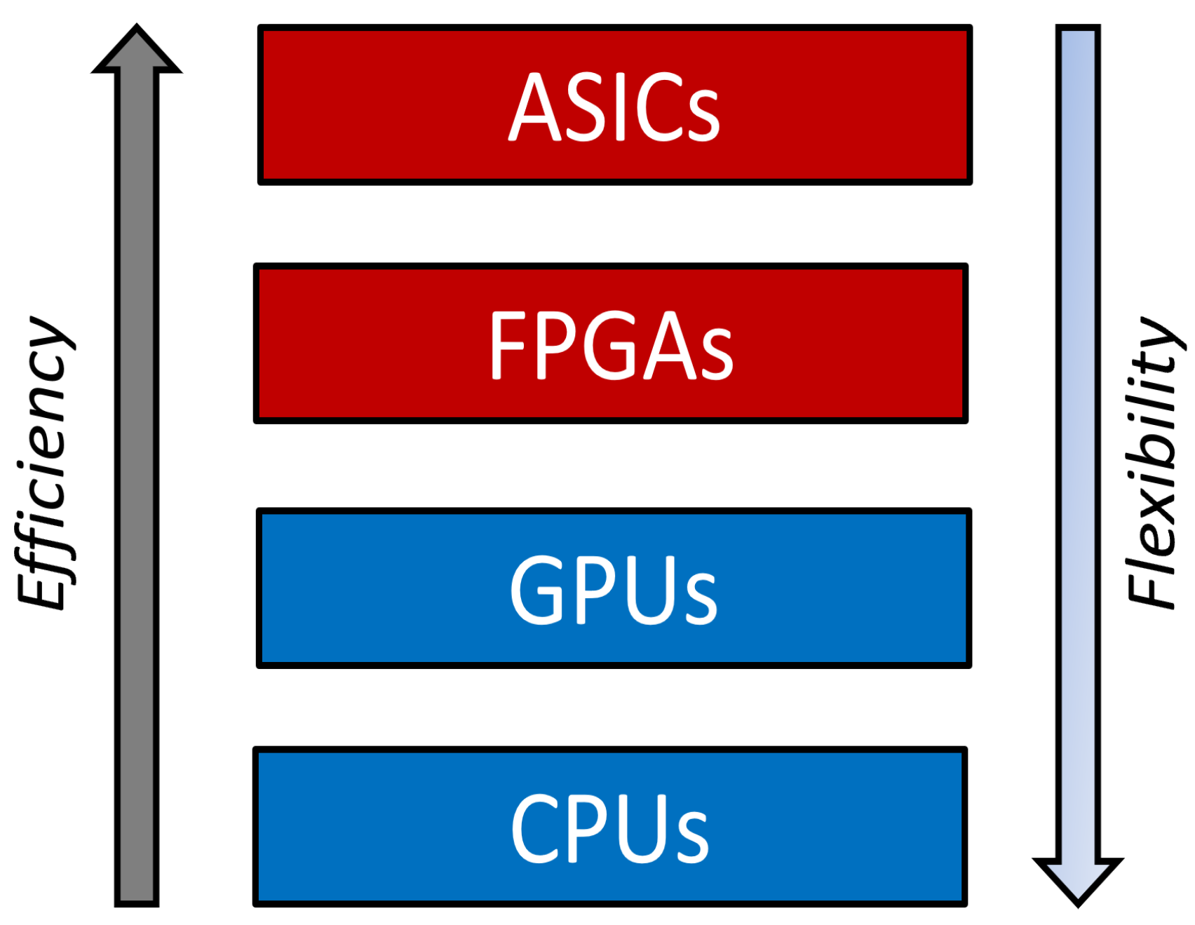
1.2. Neuromorphic Accelerators (NMAs)

As mentioned earlier, though a lot of NMAs have been presented in the literature, none of them have been specifically designed for aquaponics. Moreover, the available NMAs or the schemes they use have been designed keeping only the inference in mind. Only a few hardware systems can train SNNs [9]. Moreover, systems capable of online learning are quite complex and do not yield high accuracy.
The authors in [33], for example, present a hardware neural system that can detect epileptic seizures with 95.14% accuracy. They implement fully parallel sigmoidal neurons using look-up tables on an FPGA. A generic hardware NN system that has been tested on a digit classification dataset is presented in [22]. The system in [34] has been tested on a cancer detection dataset. The system can predict the type of cancer with 98.23% accuracy.
Again, there is no system that can perform inference in a single time step. Almost all systems require tens of time steps for inference. Systems that require fewer than 10 time steps are quite rare. The system presented in [17] is one such example; the system achieves converges in eight time steps. The basic problem with [17] is that it has been designed specifically for MNIST dataset and has not been applied to aquaponics. The system in [35] uses 100 s of time steps to achieve 89% accuracy on a binary pattern recognition dataset having six samples. Since the dataset is extremely small, the efficiency of the scheme cannot be trusted. Moreover, the efficiency of the scheme has not been evaluated on any aquaponics data.
The system in [36] uses linear STDP to simplify the proposed hardware structure. Multiple subnetworks are used instead of a grand network to achieve better accuracy. The system in [37] presents a low-power SNN system capable of online learning. The system is better than many contemporary systems but achieves only 85% accuracy on MNIST. Though the systems in [36,37] are better than many other systems in terms of hardware efficiency and accuracy, their efficiency has not been demonstrated for aquaponics. The work in [38] presents a system that is capable of training SNNs by itself. The system uses the Tempotron learning rule for SNN training. However, the Tempotron algorithm is not suitable for multiclass classification and may not be suitable for aquaponics where multiple output classes are present. The system in [39] is another example of the online SNN learning system. It uses the Tempotron learning rule for 3-class classification and uses look-up tables for post-synaptic potential (PSP) kernel computations. It uses the system for pixel classification that takes around 100 time steps.
Other examples of systems requiring tens of time steps can be seen in [40,41,42,43]. Based on all these examples, we may safely conclude that no dedicated hardware system deals with smart aquaponics. Moreover, almost all systems require tens of time steps to achieve decent accuracy and are quite costly.

Problem Definition

Fish size estimation is an important part of smart aquaponics. Such systems are generally deployed using general-purpose computers that use artificial neural networks. Since GPCs are extremely slow and ANNs are quite costly, most SASs are expensive and slow. Though spiking neural networks are more hardware-efficient than ANNs, their training process is quite complex, tricky, and time consuming. Moreover, most online learning engines based on SNNs yield low accuracy.
Therefore, the first goal is to develop a hardware-efficient SNN learning scheme for smart aquaponics. The second goal is to design a hardware engine that can support the SNN-based ‘intelligent’ part of the SAS. The proposed system can estimate the fish weight category with 99.67% accuracy and the length category with 98.03% accuracy. The hardware engine is much cheaper than most contemporary designs. This intelligent module can automate the nutrient control process, which will in turn help in maintaining a stable SAS.

2. Materials and Methods

We develop and synthesize a neural network for estimating fish length and weight. The fish size estimation results can then be sent to a controller that makes feeding decisions. The proposed network structure is shown in Figure 6. The network has 4 layers: one input layer, two hidden layers, and an output layer. The input layer has been normalized according to the procedure described in [34]. In Figure 6, the symbol N represents the number of input features, and H is a symbol for the H t h hidden neuron.
  • Forward NN Pass
The complete network has four layers: one for inputs, one for outputs, and two hidden layers for spiking computations. In this article, the i t h synaptic weight and input are denoted by W i and X i , respectively. The subscript j is for the jth postsynaptic neuron. The letter C t h represents the threshold controller, and the letter V represents the postsynaptic voltage. The postsynaptic voltage at a neuron j for the time step t is represented in Equation (1) by V j . In Equation (1), C t h j acts as a bias for ANN layers and as a dynamic threshold controller (DTC) for spiking layers. This dynamic threshold controller is learnable. The λ is the leak factor. The purpose of this leak is to allow a steady decay of the membrane potential with respect to time. This leak can enhance the level of accuracy if the noise in a system has high frequency components [44]. However, since the focus of this work is to perform all computations in a single time step, this leak term is ignored. This neuronal model is similar to the one in [17].
v j [ t ] = i W i · X i + C t h j + λ v [ t 1 ]
The inputs are normalized, as mentioned earlier. Unlike most other works on SNN such as [14,15,17], we do not convert input data into spikes. This is because the conversion to spikes is never lossless, and this can result in a severe degradation of accuracy [19]. Therefore, full-resolution inputs are applied to the network and then multiplied with corresponding synaptic efficacies, according to Equation (2). The learnable C 1 term is added as a neuronal offset for better learning. The final postsynaptic voltage is then compared against a threshold. If the given voltage is greater than this threshold, a spike is produced at the neuronal output; otherwise, nothing happens. This is described mathematically in Equation (3).
v 1 = i W i · X i + C t h 1
A 1 = 1 v 1 V t h 0 v 1 < 0
The Layer 1 activation vector is then passed as input to the Hidden Layer 2 in order to obtain the postsynaptic voltage V 2 , as represented in Equation (4).
v 2 = i W i · A 1 i + C t h 2
The Hidden Layer 1 spiking operation is repeated for the Hidden Layer 2 (HL2) as well. The spikes coming from the HL2 are applied to the output layer. However, the output layer is slightly different from the hidden layers. At the output layer, we do not perform any thresholding and use full-resolution outputs for prediction/classification. Again, the purpose is to preserve data integrity in order to produce accurate results. The thresholding operation can greatly reduce the network performance. As shown in the coming sections in detail, the full-resolution outputs do not reduce hardware efficiency at all. In fact, it can be slightly more hardware-efficient than the case where the spiking operation has to be performed in hardware since the spiking operation requires an additional comparator. At the output layer, the activated values are the same as the incoming voltage values. Therefore, the neuronal voltages are compared directly. The neuron with the maximum voltage corresponds to the predicted class, as shown in Equation (5).
A 3 = i W i · A 2 i + C t h 3
  • Backward NN Pass
As mentioned in the previous sections, the gradient of the spiking function is the diract delta function that cannot be backpropagated. In order to resolve this issue, scientists have come up with the so-called surrogate gradients that are used as a replacement of the true gradient [15,17]. Some of the famous surrogate gradients are the sigmoidal gradient, the rectangular function, the polynomial function, and the Gaussian function. Among all these functions, the rectangular function is the most hardware-efficient. However, this sometimes results in poor accuracy, as shown in Section 3. The sigmoid gradient is quite smooth; it is given in Equation (6).
d ( A j ) = 1 1 + e v j · 1 1 1 + e v j
Though the sigmoid derivative works pretty well as a surrogate gradient, it is difficult to implement in hardware since it is quite complex, as shown in Table 1. Therefore, various researchers have come up with functions that yield the same performance as the original sigmoid function while being hardware-efficient. One of the best examples that we could find in the literature is ‘Zhang–Sigmoid’ (ZS), given in [45]. The derivative of the Zhang–Sigmoid in [45] has a mean-squared error (MSD) of only 0.013% with the original sigmoidal derivative. The ZS derivative is compared with the original derivative in visual form in Figure 7. The mathematical expression is given in Equation (7).
d ( A j ) = 4 + v j 16 4 v j < 0 4 v j 16 0 v j < 4 0 o t h e r w i s e
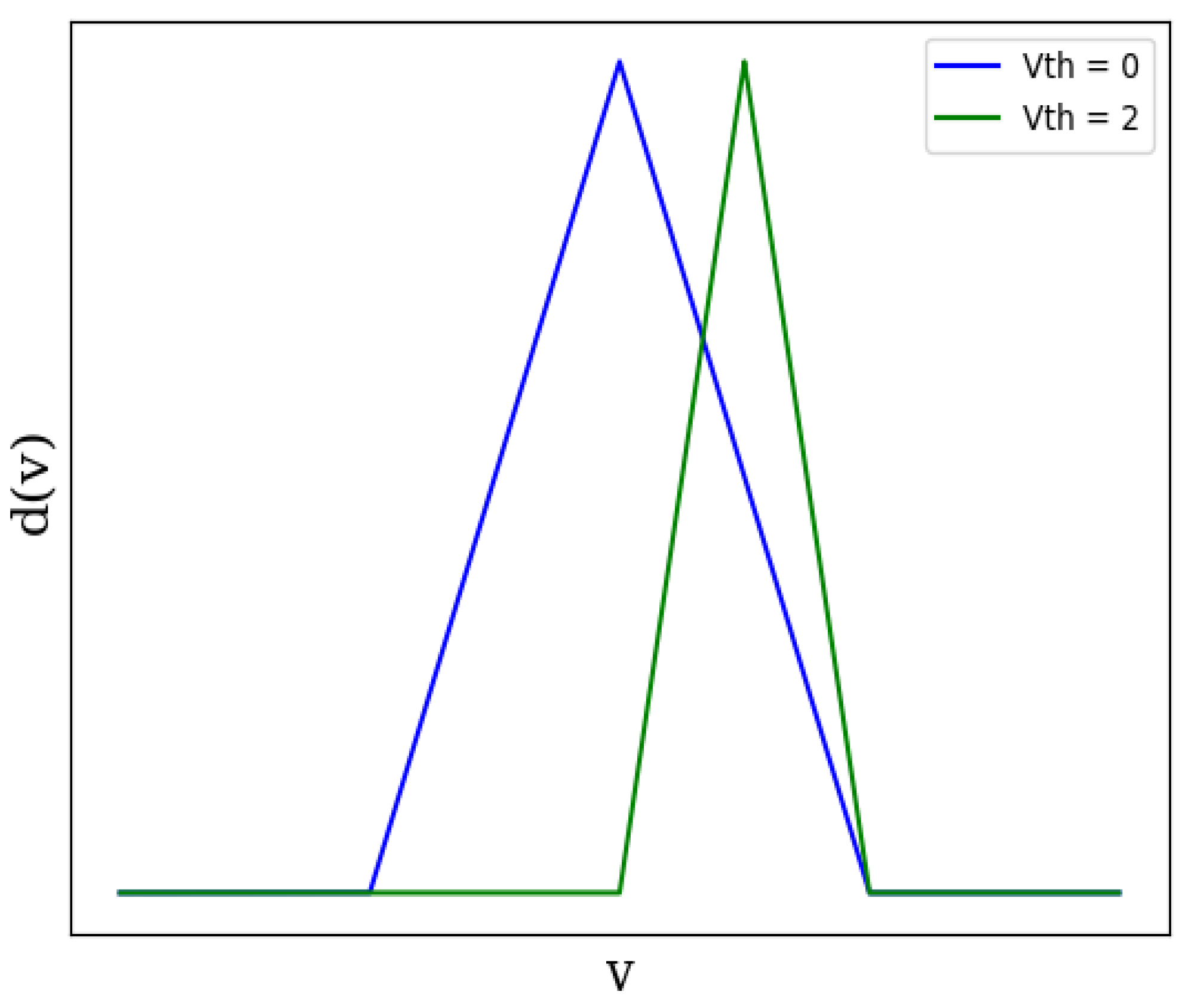
  • Proposed Surrogate Gradient
Though the original Zhang derivative/gradient apparently seems nearly perfect, a basic problem surrounding it is the lack of flexibility. The original ZS derivative cannot move and can work only when the spiking threshold voltage ( V t h ) is equal to zero, i.e., when V t h = 0 . Therefore, we proposed a modification of the original derivative so that it can work with any threshold. The proposed, generalized form of ZS derivative is given in Equation (8). By manipulating the coefficients a and V t h , it is possible to train an SNN for any threshold value. This flexibility can yield great results since the zero threshold may not work for all datasets. The choice of threshold and other such parameters can greatly affect accuracy. The value of a can be adjusted in a way that it can be implemented without using any multiplier. The impact of the changing threshold on the shape of the proposed derivative is visually represented in Figure 8. Moreover, a comparison between the proposed surrogate gradient and other modern gradients (using the number of operations as a metric) is given in Table 1. In Table 1, μ represents the Gaussian mean, σ represents the standard deviation, and fxd is a short form for ‘fixed’.
d ( A j ) = a ( 4 + v j V t h ) 16 4 a + V t h v j < V t h a ( 4 v j V t h ) 16 V t h v j < 4 a + V t h 0 o t h e r w i s e
  • Experimental and Mathematical Proofs
As discussed and proven in this segment, the proposed Spikoponic derivative (given in Equation (8)) is valid for SNN backpropagation.
  • Experimental Proof: The proposed Spikoponic derivative is used for backpropagation to train a network that classifies fish on the basis of their weight and length. Extensive experiments have been carried out using the proposed Spikoponic derivative. The details of the dataset are given in Section 3.1; the parameter values are given in Table 2. The results are given in Section 3.2. As shown in results, the proposed derivative works perfectly and can train an SNN for fish size estimation.
  • Mathematical Proof: In order to perform backpropagation, the activation function must have a finite derivative [9,15,47]. The proposed spikoponic derivative, given in Equation (8), is finite. The derivative holds valid values since it is not always equal to zero or infinity.
    Moreover, if the parameter a (in the Spikoponic derivative function) is equal to , the derivative converges to the dirac delta function, shown in Figure 5. This behavior clearly shows that the Spikoponic derivative is a valid function for the backward pass if step function is used in the forward pass. The mathematical expression for this behavior is given in Equation (9).
    d ( A j ) = v j = V t h 0 o t h e r w i s e
    The weights and DTCs are updated according to gradient descent rules, where network layers are iteratively updated based on an error function. Though all these processes are integrated into modern Python packages and we do not have to code everything in detail, we give a brief overview just to enhance readers’ understanding. The two basic parameter update rules are given in (10) and (11).
    W ( l ) + W l η L W l
    C th ( l ) + C th l η L C th l
    In the above equations, W l represents ‘weight vector’ and C t h l represents the DTC vector at layer l. Here, η represents the learning rate, the parameter that determines the speed at which the network updates weights in a training iteration. The term L W l describes the changes in loss function with respect to weights at layer l. Both these terms are calculated using the chain rule, as in [9,15,17].
    Since there are multiple layers in the proposed network, it would be unnecessary to derive mathematical expressions for all the layers. Therefore, we derive expressions only for one layer as a reference, just to give an idea of how the system works. Expressions for other layers can be derived using the same principle.
    We mathematically establish the dependence of loss functions ( L ) on Layer 2 synaptic strengths in Equation (12), and on Layer 2 DTC ( C t h 2 ) in Equation (13). To make the analysis understandable, the mean squared error (MSE) function has been used for reference. In the following equations, A 3 is the obtained output value at Layer 3, and y is the label voltage. The Spikoponic derivative function is already given in Equation (8). In order to keep mathematics simple, we do not incorporate terms associated with the optimization methhods such as ADAM [48] in the presented mathematical expressions. Equations (12) and (13) do not incorporate the temporal dependence of the network parameters and have been derived for one time step, which is one of the main goals of this work. To ignore temporal dependence, we make λ equal to zero.
    L W 2 = A 1 W 3 ( A 3 y ) ( a ( 4 + v 2 V t h ) ) 16 4 a + V t h v 2 < V t h A 1 W 3 ( A 3 y ) ( a ( 4 v 2 V t h ) ) 16 V t h v 2 < 4 a + V t h 0 o t h e r w i s e
    L C th 2 = C t h 2 W 3 ( A 3 y ) ( a ( 4 + v 2 V t h ) ) 16 4 a + V t h v 2 < V t h C t h 2 W 3 ( A 3 y ) ( a ( 4 v 2 V t h ) ) 16 V t h v 2 < 4 a + V t h 0 o t h e r w i s e
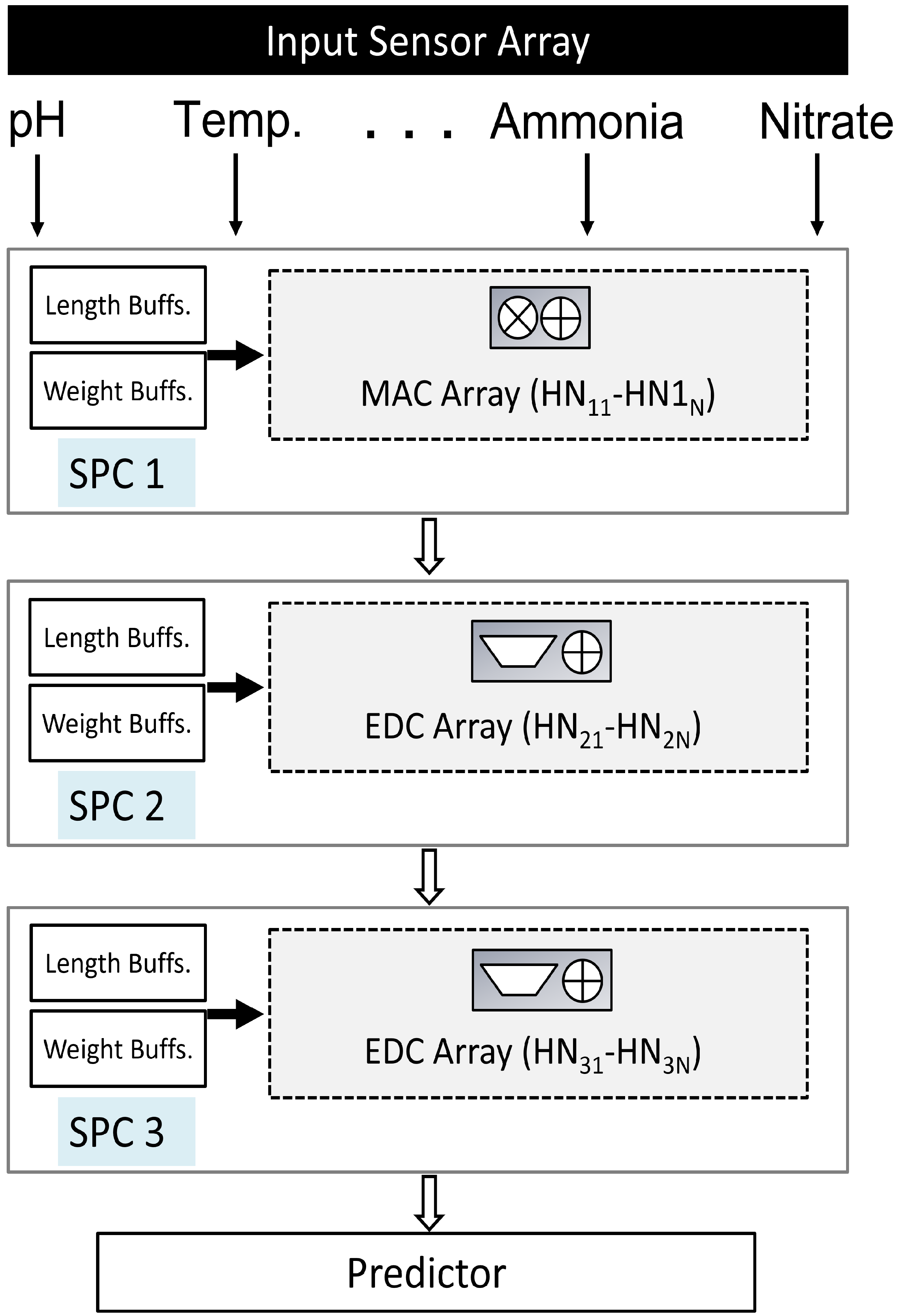
  • Proposed SpikoPoniC Hardware Engine
The proposed hardware system takes input from eight different sensors (systems), responsible for computing the following parameters: pH, temperature, date of creation, turbidity, dissolved oxygen, ammonia, nitrate, and population size. The system is fully parallel and can predict eight levels of fish weight and length (based on the input data) in a single clock cycle. The system consists of an input layer, two event-driven SNN layers, and an output layer containing a predictor. There are six different memory buffers, two for each layer. The top level diagram of the complete system is shown in Figure 9. The details of each of the components are mentioned in the coming subsections.

2.1. Switching Buffers

Since the system can estimate both length and weight categories, there are two types of memory buffers available for every network layer: one for storing synaptic efficacies corresponding to fish weight and the other one for storing efficacies corresponding to length. Which memory buffers are to be activated depends on the user. If length is to predicted, the length memory buffers (LMBs) are enabled, weight memory buffers (WMBs) are disabled, and vice versa. Upon selection, all the synaptic efficacies are fetched in parallel to obtain high throughput.

2.2. Event-Driven Spiking Computers (EDCs)—Hidden Layer 1

As mentioned earlier, the first layer receives normalized inputs from sensors. These inputs are multiplied by the corresponding synaptic efficacies (SEs) in order to obtain voltage. The multiplications can be carried out using DSP48 elements on the FPGA. The voltage is obtained using a pipelined adder tree; the purpose of pipelining is to increase throughput. The first layer synaptic operations are, therefore, typical multiply accumulate (MAC) operations.
If the voltage is greater than a pre-defined threshold, a 1-bit spike is emitted; otherwise, nothing is passed. This is done using a comparator (CMP). Finally, these 1-bit values are stored in a pipeline register in order to increase throughput. Since spikes are quite small in size (1 bit), the pipeline register has a very small footprint. The spikes are then sent to the subsequent layer EDCs. The structure of a Layer 1 EDC is shown in Figure 10.

2.3. EDCs—Hidden Layer 2

The spikes coming from the HL1 are provided as input to the HL2. The HL2 actuators are also event-driven in nature, i.e., they are activated only when there is a valid spike coming from the previous layer. If there is no spike, no processing takes place by the processing elements and zero voltage is passed on to the subsequent unit. If there is a spike, the respective synaptic efficacy gets added up to other valid synaptic efficacies by a pipelined adder tree.
The structure of the HL2 EDCs is shown in Figure 11. Like HL1, both the length and weight buffers are present. Once all the valid synaptic efficacies have been added up by the voltage computer (adder tree), a comparison operation is performed on the final voltage. If the voltage is greater than a predefined threshold, a spike is produced; otherwise, nothing happens. These spikes are then stored in the HL2 spike register that acts like a pipeline register. The outputs emanating from the spike register are then applied as input to the output layer.

2.4. Output-Layer EDCs

The structure of output-layer NACs is shown in Figure 12. Since softmax is a costly function and is used only when cross entropy loss is to be visualized, we use logits to perform prediction at the output [22]. The maximum voltage neuron corresponds to the predicted class. No spikes are used at the output for two reasons: the use of spikes results in a degradation of accuracy; an extra comparator is required. Therefore, the predictor directly compares logits and selects the one with the maximum value.

3. Results and Discussion

This section presents the algorithmic and hardware efficiency of SpikoPoniC. The SpikoPoniC is compared with both software- and hardware-based works under the predefined test conditions. The FPGA-based SpikoPoniC is first compared with the CPU based aquaponic neural system in terms of speed for the same level of accuracy and then with other FPGA-based works in terms of cost and throughput.

3.1. Benchmarks and Test Conditions

The hardware inference system SikoPoniC—implemented on Virtex 6 (xc6vlx75t-ff784)—uses 7-bit synaptic efficacies and dynamic threshold controllers. The training has been performed on a GPC for the following NN topology: eight inputs; two hidden layers, each having 16 neurons; and eight output neurons. Python has been used for algorithmic evaluations, and Verilog has been used for hardware modeling. Since the platform is Virtex 6, the maximum temperature at which the device can operate is 85 degrees celsius [49]. Each 64 bit-wide block RAM can generate, store, and utilize eight additional Hamming-code bits and perform single-bit error correction and double-bit error detection (ECC) during the read process. As a special option, the bitstream can be AES-encrypted to prevent unauthorized copying of the design [49].
The dataset used is available from [50]. Since the directory contains a lot of files, only one file, which contains 175,000 samples, is sufficient for reliable performance evaluation. About 150k samples are used for training, and 25k are used for testing. There are 32 samples in a batch. The learning rate is 0.001, by default. The scheme uses the ADAM optimizer [48]. Backpropagation is performed using the cross entropy loss function. The system converges in about 47 epochs. Table 2 presents the test conditions and hyper-parameter values used for evaluating SpikoPoniC. For hyper-parameter tuning, we use grid search [51].

3.2. Algorithmic Efficiency Evaluation and Comparisons

The amount of CPU time that a training epoch consumes in the proposed scheme is shown in Figure 13. The average time per epoch is around 5 s. Once the network has been trained, the CPU uses approximately 1 s to infer all (≈25,000) the test samples.
The proposed system can estimate the range of fish weight with 99.67% accuracy and the range of fish length with 98.03% accuracy. The average fish size estimation accuracy, therefore, is 98.85% accurate. The accuracy as a function of the number of epochs is shown in Figure 16; this figure is shown in the later part of this subsection along with all the necessary details. A comparison of SpikoPoniC with various modern DL-based aquaponic monitoring schemes in terms of accuracy is given in Table 3.
For fish weight estimation, the maximum precision and recall values are 94.80% and 99.88%, respectively. For fish length estimation, the maximum precision and recall values are 88.39% and 99.30%, respectively. On average, an F1 score of 93.701% can easily be obtained when it comes to fish size (which includes both length and weight) estimation. It is not possible to compare our results with other works in terms of precision, recall, or F1 score. This is because many research works on aquaponics do not use these metrics and rely on accuracy for performance evaluation.
A visual comparison in the form of bar graphs between various algorithms for fish weight and length estimation is given in Figure 14. The following algorithms are compared in Figure 14. All the algorithms are applied for just one time step.
  • Direct SNN Training (DST) [15,17].
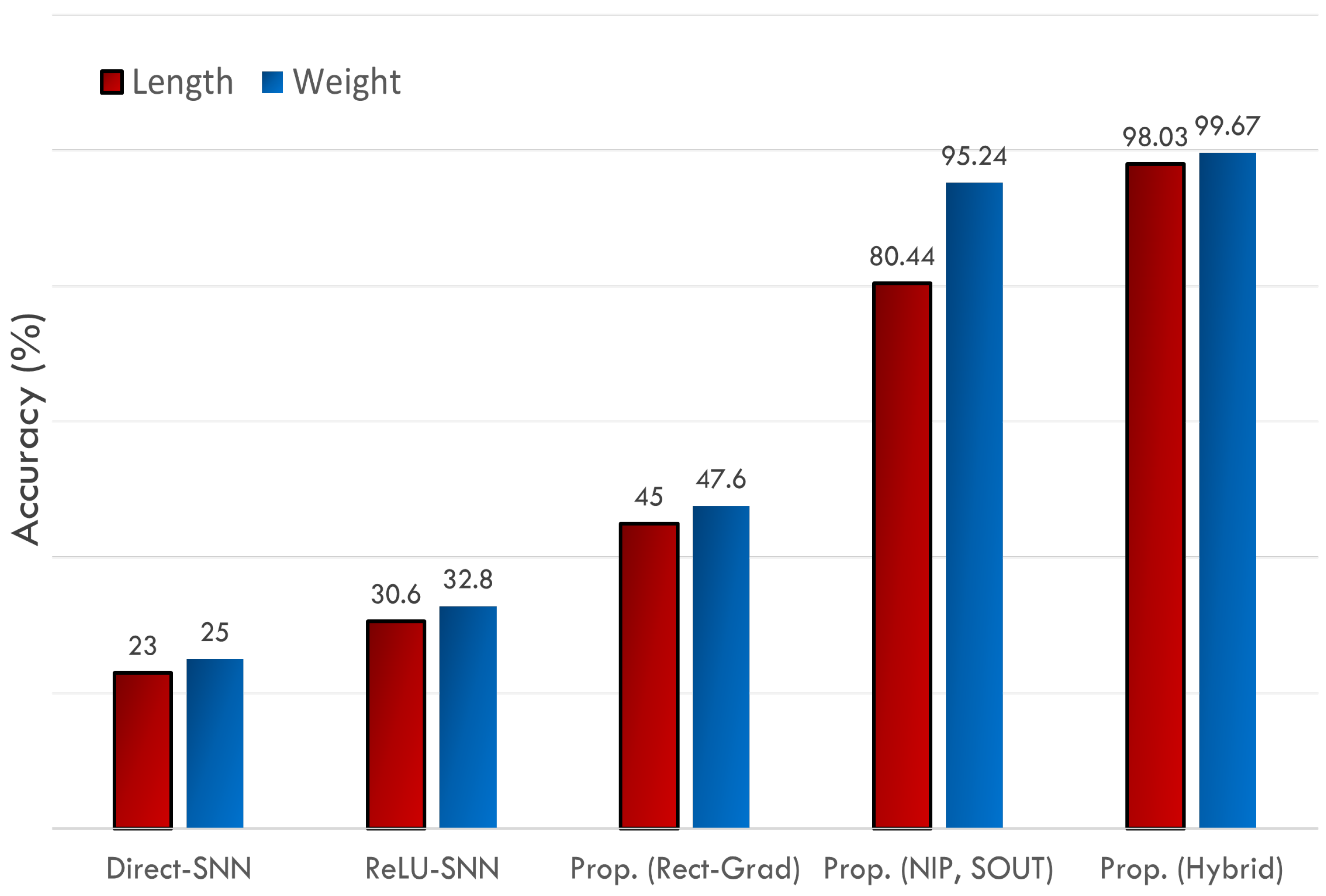
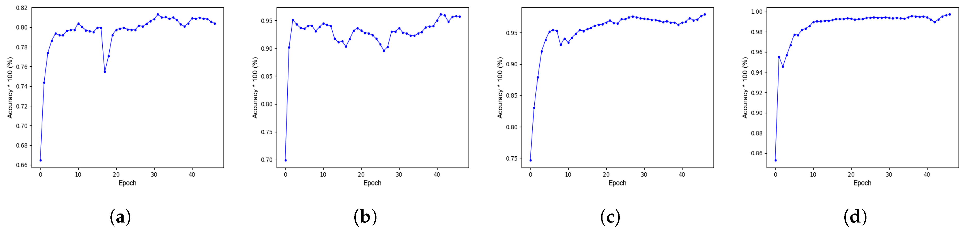
    All the layers use spikes in the forward pass and surrogate gradient (sigmoidal gradient [15]) in the backward pass. The network achieves very low accuracy since there is only one time step for which we have to train the network.
  • ReLU-SNN Conversion (ReLU-SNN) [19].
    The network is trained using ReLU function, and the trained network is then converted into an SNN. No weight-threshold normalization is applied since the purpose is to devise an algorithm that is hardware-efficient if on-chip learning is required. Normalization processes can never be efficient for on-chip learning [9]. For better accuracy, the inputs are not converted into spikes since this results in a loss of accuracy [19].
  • Rectangular Straight-Through Estimator (Rect-STE) [17].
    The network uses spikes in the forward pass, and the rectangular-shaped surrogate gradient in the backward pass, as in [17]. For achieving high accuracy, full-resolution inputs are used and no conversion to spikes takes place.
  • Proposed Algorithm (Normalized Inputs, Spiking Outputs).
    The proposed algorithm, as mentioned in Section 2, is applied with full-resolution inputs but spiking outputs.
  • Proposed Algorithm (Normalized Inputs, Full-Resolution Outputs).
    The proposed algorithm, as described in Section 2, is applied with full-resolution inputs and outputs (logits).
The results are presented in Figure 14. All schemes other than the proposed one yield poor results. Let us discuss the underlying causes. The DST, ReLU-SNN, and Rect-STE are strongly dependent on a large time period since they all use spikes at both the input and the output layers. Though the use of spikes at the input layer is quite hardware-efficient, it results in a degradation of accuracy due to the loss incurred in the conversion process. As a result, good accuracy cannot be obtained in a single time step. The ReLU-SNN scheme depends strongly on weight-threshold balancing too [18]. For the proposed scheme, the use of spikes at the output layer results in a lower accuracy than the case where logits (voltage as such) are used at the output layer. The simple reason is that the conversion of voltage into 1-bit spikes even at the output layer reduces the dynamic range and precision, resulting in visible loss of accuracy. Moreover, as explained in the coming sections, the use of raw voltage instead of converted spikes at the output layer does not decrease hardware efficiency at all.
As mentioned earlier, the use of spikes at both the input and output layers for a single time step does not produce good results. This is evident even from Figure 15a, which shows the evolution of training accuracy with the number of training epochs: the fluctuation is very high and there is no such thing as convergence. Similarly, the use of rectangular, flat surrogate gradient results in a very poor accuracy. In fact, no convergence is achieved since the gradient is completely flat and can result in gradient vanishing/explosion. The rectangular gradient does not change its shape and fails to fit for complex data. The sigmoidal gradient, on the other hand, does change its shape around the threshold and results in better learning.
The use of full-resolution inputs and outputs, instead of spikes, preserves the data content and produces excellent results. The results obtained using the proposed algorithm for fish length and weight estimation are shown in Figure 16c and Figure 16d, respectively. As shown in the figures, the network learning is quite smooth. However, if spikes are used even at the output layer, the accuracy degrades and network accuracy keeps fluctuating. This is shown in Figure 16a,b.

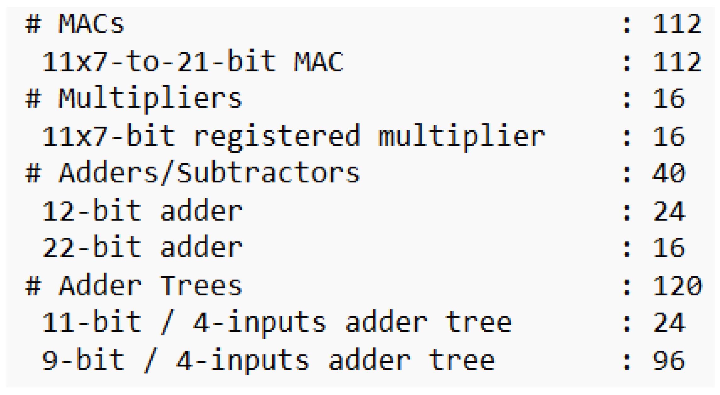
3.3. Hardware Efficiency Evaluation and Comparisons

SpikoPoniC is fully parallel and can process a single sample in a single clock cycle. The maximum attainable clock frequency is 84.23 MHz to 117.33 MHz, depending on the type of implementation and hardware synthesizer settings, as will be discussed later. SpikoPoniC can process more than 84 million samples in a second. A comparison between the FPGA and CPU implementations is given in Figure 17, which shows that the FPGA system is at least 3369 times faster than the CPU implementation. In Figure 17, the throughput is given in terms of millions of samples per second (MSPS). This shows the potential of neurormophic systems and provides a great incentive to SAS developers. For the SpikoPoniC, the results have been obtained with and without using DSP48 elements. At the given frequencies, the DSP implementation consumes about 1.975 watts, of which the leakage power is around 1.577 watts; the non-DSP implementation consumes about 2.302 watts, of which the leakage power is around 1.582 watts.
A comparison between the fully ANN implementation and the proposed SNN (hybrid) implementation for the same test topology (30-5-5-2) under the same test conditions is shown in Figure 18. As shown in Figure 18, the proposed implementation is far better than the ANN implementation in terms of latency (speed) and cost (amount of FPGA resources occupied). Compared with the proposed technique, the fully ANN implementation consumes approximately 27% more registers, 45% look-up tables, and 28% more time. The disparity will grow as the network becomes deeper and larger. The purpose of this figure is to give a glimpse into the disparity between the proposed implementation and the fully ANN implementation. The network accuracy, however, remains (more or less) the same. For example, in the finalized network, discussed in Table 4, the proposed scheme incurs less than 1% loss, compared to the actual ANN scheme using rectified linear units (ReLUs) at all the layers in the context of fish length estimation. For fish weight estimation, there is no difference at all between the proposed scheme and the ANN-based scheme. There is a reason why we chose 30-5-5-2 topology for ANN-SNN hardware efficiency comparison: the available hardware platform is a low-end model of Virtex 6 (xc6vlx75t-ff784) which has approximately 93,000 slice registers and about 46,000 look-up tables only. A large, fully parallel ANN design cannot fit on such a small platform, given the limited amount of resources. The ANN implementation for a large topology, say 8-16-16-8, is unable to fit on the given platform, though an SNN implementation for the same topology is possible. This simply proves that the SNN implementation is more efficient on hardware than the ANN one.
Figure 19 shows the number of adders and multipliers required by the proposed implementation. The cost and throughput comparisons are given in Table 4.
For the SpikoPoniC, the results have been obtained with and without using DSP48 elements. In both the cases, SpikoPoniC shows superior performance. Though the systems presented in Table 4 are quite hardware-efficient, they suffer from one or both of the following problems: the systems are not made specifically for aquaponics, or the systems are quite costly because they are based on ANNs. For example, the system in [33] has been developed for diagnosing epilepsy. Moreover, the system uses parallel sigmoidal neurons, which are quite costly to be used on hardware. The system predicts epilepsy with 95.14% accuracy. The hardware system [34] uses hardware-aware sigmoidal and swish neurons to predict cancer with high accuracy. The system in [56] implements a network with radial basis functions just to demonstrate the efficiency of slope-based Gaussian approximation; no dataset is used to evaluate performance. The system in [22] uses ReLU at all the network layers to to improve classification accuracy. However, it uses extremely small weights and biases, which might not be enough for obtaining a reasonable accuracy on aquaponics data. Furthermore, the system does not use any aquaponics data for system evaluation. Therefore, how it will perform on aquaponics data remains dubious.
Though the inference engine in [9] achieves a very high throughput and is cost effective, it uses spikes at all the layers. Therefore, it cannot be used for the SAS under consideration, as mentioned earlier. The data under consideration requires full resolution inputs and outputs; otherwise, it produces a very low accuracy. The work in [35] uses a small (toy) dataset with 25 binary input pixels and one neuron for binary (X and O) classification; two samples are used for training. The authors do not mention the system throughput explicitly. However, it is safe to assume that the maximum TP is far less than 1.9 × 10 6 samples per second. This is because the maximum operating frequency of the system is around 189 MHz, and the time period requires one to compute a sample is 100 ms. Moreover, the discretization step is 0.001. There is another metric used to compare these works: processing time per second (PTPS), represented in microseconds ( μ s). PTPS is the amount of time required to infer/process a given input sample. The smaller the PTPS value, the faster the system.
Table 4. Hardware cost and throughput comparisons.
SystemApplicationTopologyAccur.Regs.LuTsDSPsPlatformTPPTPS
( × 10 6 )( μ s)
 [33]Epilepsy Det.5-12-395.14%11412,960116Cyclone IV500.02
[34]Cancer Det.30-5-298.23%9832654234Virtex 663.50.0157
[22]Digit Class.64-20-1094.28%467730,6540Virtex 693.20.0107
[35]Bin. Class.25-5-189%102311,339-Virtex 6 < < 1.89>0.53
[57]None5-5-2-18983124154Virtex 5--
[56]None--790119514Spartan 3100.1
Prop. D S P Aquaponics8-16-16-898.85%10913749128Virtex 684.230.012
Prop. N O D S P Aquaponics8-16-16-898.85%425918,2830Virtex 6117.330.008

4. Conclusions

This article presents a novel training methodology to train and implement a spiking neural neural network on a neuromorphic system for smart aquaponics. The article also presents a novel surrogate gradient for SNN training that promises both flexibility and hardware efficiency.
The purpose of developing this system is the low-cost, real-time estimation of fish size, which in turn will help devise efficient smart aquaponic systems and make appropriate feeding decisions. The hardware inference engine is capable of classifying more than 84 million samples in a second. The system is trained using 150,000 samples and can predict fish length with 98.03% accuracy and fish weight with 99.67% accuracy. The design occupies only 1100 slice registers and 3749 look-up tables. The engine is about 3369 times faster than a typical GPC and is far less costly than the implementation that uses an ANN for the same job. The ANN implementation is 45% costlier than the proposed implementation with less than 1% degradation in accuracy. The system consumes about XYZ milliwatts at the maximum possible frequency, i.e., 84.23 MHz. All these results have been obtained on a low-end Virtex 6 FPGA. The maximum temperature at which the device can operate is 85 degrees celsius.
Therefore, it may safely be concluded that the proposed scheme is suitable for DL-based smart aquaponics. The scheme gives a roadmap on how to use SNNs for Aquaponics 4.0 industrial applications. In future, the same technique can be modified to be extended to spiking convolutional neural networks for better classification. Another possible improvement is to use a higher number of input features to obtain better results. A larger number of sensors can be used to collect data for application at the input side.

Author Contributions

Conceptualization, A.S. and M.A.I.; methodology, A.S.; software, A.S. and J.S.; validation, A.S. and J.S.; formal analysis, A.S.; investigation, A.S.; resources, M.A.I.; writing—original draft preparation, A.S.; writing—review and editing, A.S., M.I.V. and M.A.I.; visualization, A.S. and M.A.I.; supervision, M.I.V., M.A.I. and S.H.P.; project administration, M.I.V., M.A.I. and K.J.H.; and funding acquisition, K.J.H. and M.I.V. All authors have read and agreed to the published version of the manuscript.

Funding

The authors would like to acknowledge the financial support from the following organizations: Zuhai UM Science and Technology Research Institute, via the projects of the ZUMRI-Lingyange Semiconductor Joint Lab (CP-031-2022); the Lingyange Semiconductor Incorporated, Zhuhai (CP-017-2022); and the Blue Ocean Smart System (Nanjing) Limited (CP-003-2023).

Institutional Review Board Statement

This study does not involve humans or animals. There are no ethical concerns regarding this study.

Data Availability Statement

All the datasets used for the evaluation of the proposed scheme are available publicly. The relevant references have already been mentioned in the bibliography.

Conflicts of Interest

The authors declare no competing interests.

Abbreviations

The following abbreviations are used in this manuscript:
ANNArtificial neural network
ASICApplication-specific integrated circuit
DLDeep learning
FPGAField programmable gate array
GPCGeneral-purpose computer
SASSmart aquaponic system
SNNSpiking neural network

References

  1. Calone, R.; Orsini, F. Aquaponics: A Promising Tool for Environmentally Friendly Farming. Front. Young Minds 2022, 10, 707801. [Google Scholar] [CrossRef]
  2. Taha, M.F.; ElMasry, G.; Gouda, M.; Zhou, L.; Liang, N.; Abdalla, A.; Rousseau, D.; Qiu, Z. Recent Advances of Smart Systems and Internet of Things (IoT) for Aquaponics Automation: A Comprehensive Overview. Chemosensors 2022, 10, 303. [Google Scholar] [CrossRef]
  3. Dhal, S.B.; Jungbluth, K.; Lin, R.; Sabahi, S.P.; Bagavathiannan, M.; Braga-Neto, U.; Kalafatis, S. A machine-learning-based IoT system for optimizing nutrient supply in commercial aquaponic operations. Sensors 2022, 22, 3510. [Google Scholar] [CrossRef]
  4. Lu, H.; Ma, X. Hybrid decision tree-based machine learning models for short-term water quality prediction. Chemosphere 2020, 249, 126169. [Google Scholar] [CrossRef]
  5. Jalal, A.; Salman, A.; Mian, A.; Shortis, M.; Shafait, F. Fish detection and species classification in underwater environments using deep learning with temporal information. Ecol. Inform. 2020, 57, 101088. [Google Scholar] [CrossRef]
  6. Hasan, N.; Ibrahim, S.; Aqilah Azlan, A. Fish diseases detection using convolutional neural network (CNN). Int. J. Nonlinear Anal. Appl. 2022, 13, 1977–1984. [Google Scholar]
  7. Ubina, N.; Cheng, S.C.; Chang, C.C.; Chen, H.Y. Evaluating fish feeding intensity in aquaculture with convolutional neural networks. Aquac. Eng. 2021, 94, 102178. [Google Scholar] [CrossRef]
  8. Merolla, P.A.; Arthur, J.V.; Alvarez-Icaza, R.; Cassidy, A.S.; Sawada, J.; Akopyan, F.; Jackson, B.L.; Imam, N.; Guo, C.; Nakamura, Y.; et al. A million spiking-neuron integrated circuit with a scalable communication network and interface. Science 2014, 345, 668–673. [Google Scholar] [CrossRef]
  9. Siddique, A.; Vai, M.I.; Pun, S.H. A low cost neuromorphic learning engine based on a high performance supervised SNN learning algorithm. Sci. Rep. 2023, 13, 6280. [Google Scholar] [CrossRef]
  10. Kim, S.; Park, S.; Na, B.; Yoon, S. Spiking-YOLO: Spiking neural network for energy-efficient object detection. In Proceedings of the AAAI Conference on Artificial Intelligence, New York, NY, USA, 7–12 February 2020; Volume 34, pp. 11270–11277. [Google Scholar]
  11. Maass, W.; Papadimitriou, C.H.; Vempala, S.; Legenstein, R. Brain computation: A computer science perspective. Comput. Softw. Sci. 2019, 10000, 184–199. [Google Scholar]
  12. Izhikevich, E.M. Which model to use for cortical spiking neurons? IEEE Trans. Neural Netw. 2004, 15, 1063–1070. [Google Scholar] [CrossRef]
  13. Izhikevich, E.M. Simple model of spiking neurons. IEEE Trans. Neural Netw. 2003, 14, 1569–1572. [Google Scholar] [CrossRef]
  14. Han, J.; Li, Z.; Zheng, W.; Zhang, Y. Hardware implementation of spiking neural networks on FPGA. Tsinghua Sci. Technol. 2020, 25, 479–486. [Google Scholar] [CrossRef]
  15. Wu, Y.; Deng, L.; Li, G.; Zhu, J.; Shi, L. Spatio-temporal backpropagation for training high-performance spiking neural networks. Front. Neurosci. 2018, 12, 331. [Google Scholar] [CrossRef]
  16. Qiao, G.; Hu, S.; Chen, T.; Rong, L.; Ning, N.; Yu, Q.; Liu, Y. STBNN: Hardware-friendly spatio-temporal binary neural network with high pattern recognition accuracy. Neurocomputing 2020, 409, 351–360. [Google Scholar] [CrossRef]
  17. Yin, S.; Venkataramanaiah, S.K.; Chen, G.K.; Krishnamurthy, R.; Cao, Y.; Chakrabarti, C.; Seo, J. Algorithm and hardware design of discrete-time spiking neural networks based on back propagation with binary activations. In Proceedings of the 2017 IEEE Biomedical Circuits and Systems Conference (BioCAS), Torino, Italy, 19–21 October 2017; pp. 1–5. [Google Scholar] [CrossRef]
  18. Diehl, P.U.; Neil, D.; Binas, J.; Cook, M.; Liu, S.C.; Pfeiffer, M. Fast-classifying, high-accuracy spiking deep networks through weight and threshold balancing. In Proceedings of the 2015 International Joint Conference on Neural Networks (IJCNN), Killarney, Ireland, 12–17 July 2015; pp. 1–8. [Google Scholar]
  19. Rueckauer, B.; Lungu, I.A.; Hu, Y.; Pfeiffer, M.; Liu, S.C. Conversion of continuous-valued deep networks to efficient event-driven networks for image classification. Front. Neurosci. 2017, 11, 682. [Google Scholar] [CrossRef]
  20. Azghadi, M.R.; Lammie, C.; Eshraghian, J.K.; Payvand, M.; Donati, E.; Linares-Barranco, B.; Indiveri, G. Hardware implementation of deep network accelerators towards healthcare and biomedical applications. IEEE Trans. Biomed. Circuits Syst. 2020, 14, 1138–1159. [Google Scholar] [CrossRef]
  21. Ortega-Zamorano, F.; Jerez, J.M.; Urda Muñoz, D.; Luque-Baena, R.M.; Franco, L. Efficient Implementation of the Backpropagation Algorithm in FPGAs and Microcontrollers. IEEE Trans. Neural Netw. Learn. Syst. 2016, 27, 1840–1850. [Google Scholar] [CrossRef]
  22. Siddique, A.; Iqbal, M.A.; Aleem, M.; Islam, M.A. A 218 GOPS neural network accelerator based on a novel cost-efficient surrogate gradient scheme for pattern classification. Microprocess. Microsyst. 2023, 99, 104831. [Google Scholar] [CrossRef]
  23. Junior, A.d.S.O.; Sant’Ana, D.A.; Pache, M.C.B.; Garcia, V.; de Moares Weber, V.A.; Astolfi, G.; de Lima Weber, F.; Menezes, G.V.; Menezes, G.K.; Albuquerque, P.L.F.; et al. Fingerlings mass estimation: A comparison between deep and shallow learning algorithms. Smart Agric. Technol. 2021, 1, 100020. [Google Scholar] [CrossRef]
  24. Ren, Q.; Zhang, L.; Wei, Y.; Li, D. A method for predicting dissolved oxygen in aquaculture water in an aquaponics system. Comput. Electron. Agric. 2018, 151, 384–391. [Google Scholar] [CrossRef]
  25. Diehl, P.U.; Cook, M. Unsupervised learning of digit recognition using spike-timing-dependent plasticity. Front. Comput. Neurosci. 2015, 9, 99. [Google Scholar] [CrossRef] [PubMed]
  26. Saunders, D.J.; Siegelmann, H.T.; Kozma, R. STDP learning of image patches with convolutional spiking neural networks. In Proceedings of the 2018 International Joint Conference on Neural Networks (IJCNN), Rio de Janeiro, Brazil, 8–13 July 2018; pp. 1–7. [Google Scholar]
  27. Vicente-Sola, A.; Manna, D.L.; Kirkland, P.; Di Caterina, G.; Bihl, T. Keys to accurate feature extraction using residual spiking neural networks. Neuromorphic Comput. Eng. 2022, 2, 044001. [Google Scholar] [CrossRef]
  28. Deng, S.; Gu, S. Optimal conversion of conventional artificial neural networks to spiking neural networks. arXiv 2021, arXiv:2103.00476. [Google Scholar]
  29. Fang, W.; Yu, Z.; Chen, Y.; Huang, T.; Masquelier, T.; Tian, Y. Deep residual learning in spiking neural networks. Adv. Neural Inf. Process. Syst. 2021, 34, 21056–21069. [Google Scholar]
  30. Zhang, W.; Li, P. Temporal spike sequence learning via backpropagation for deep spiking neural networks. Adv. Neural Inf. Process. Syst. 2020, 33, 12022–12033. [Google Scholar]
  31. Tavanaei, A.; Maida, A. BP-STDP: Approximating backpropagation using spike timing dependent plasticity. Neurocomputing 2019, 330, 39–47. [Google Scholar] [CrossRef]
  32. Tavanaei, A.; Kirby, Z.; Maida, A.S. Training spiking convnets by stdp and gradient descent. In Proceedings of the 2018 International Joint Conference on Neural Networks (IJCNN), Rio de Janeiro, Brazil, 8–13 July 2018; pp. 1–8. [Google Scholar]
  33. Sarić, R.; Jokić, D.; Beganović, N.; Pokvić, L.G.; Badnjević, A. FPGA-based real-time epileptic seizure classification using Artificial Neural Network. Biomed. Signal Process. Control 2020, 62, 102106. [Google Scholar] [CrossRef]
  34. Siddique, A.; Iqbal, M.A.; Aleem, M.; Lin, J.C.W. A high-performance, hardware-based deep learning system for disease diagnosis. PeerJ Comput. Sci. 2022, 8, e1034. [Google Scholar] [CrossRef]
  35. Farsa, E.Z.; Ahmadi, A.; Maleki, M.A.; Gholami, M.; Rad, H.N. A low-cost high-speed neuromorphic hardware based on spiking neural network. IEEE Trans. Circuits Syst. II Express Briefs 2019, 66, 1582–1586. [Google Scholar] [CrossRef]
  36. Sun, C.; Sun, H.; Xu, J.; Han, J.; Wang, X.; Wang, X.; Chen, Q.; Fu, Y.; Li, L. An Energy Efficient STDP-Based SNN Architecture With On-Chip Learning. IEEE Trans. Circuits Syst. I Regul. Pap. 2022, 69, 5147–5158. [Google Scholar] [CrossRef]
  37. Li, S.; Zhang, Z.; Mao, R.; Xiao, J.; Chang, L.; Zhou, J. A Fast and Energy-Efficient SNN Processor With Adaptive Clock/Event-Driven Computation Scheme and Online Learning. IEEE Trans. Circuits Syst. I Regul. Pap. 2021, 68, 1543–1552. [Google Scholar] [CrossRef]
  38. Siddique, A.; Vai, M.I.; Pun, S.H. A low-cost, high-throughput neuromorphic computer for online SNN learning. Clust. Comput. 2023, 1–18. [Google Scholar] [CrossRef]
  39. Zhang, G.; Li, B.; Wu, J.; Wang, R.; Lan, Y.; Sun, L.; Lei, S.; Li, H.; Chen, Y. A low-cost and high-speed hardware implementation of spiking neural network. Neurocomputing 2020, 382, 106–115. [Google Scholar] [CrossRef]
  40. Heidarpur, M.; Ahmadi, A.; Ahmadi, M.; Azghadi, M.R. CORDIC-SNN: On-FPGA STDP learning with izhikevich neurons. IEEE Trans. Circuits Syst. I Regul. Pap. 2019, 66, 2651–2661. [Google Scholar] [CrossRef]
  41. Lammie, C.; Hamilton, T.; Azghadi, M.R. Unsupervised character recognition with a simplified FPGA neuromorphic system. In Proceedings of the 2018 IEEE International Symposium on Circuits and Systems (ISCAS), Florence, Italy, 27–30 May 2018; pp. 1–5. [Google Scholar]
  42. Ma, D.; Shen, J.; Gu, Z.; Zhang, M.; Zhu, X.; Xu, X.; Xu, Q.; Shen, Y.; Pan, G. Darwin: A neuromorphic hardware co-processor based on spiking neural networks. J. Syst. Archit. 2017, 77, 43–51. [Google Scholar] [CrossRef]
  43. Neil, D.; Liu, S.C. Minitaur, an event-driven FPGA-based spiking network accelerator. IEEE Trans. Very Large Scale Integr. (VLSI) Syst. 2014, 22, 2621–2628. [Google Scholar] [CrossRef]
  44. Chowdhury, S.S.; Lee, C.; Roy, K. Towards Understanding the Effect of Leak in Spiking Neural Networks. arXiv 2020, arXiv:2006.08761. [Google Scholar] [CrossRef]
  45. Zhang, M.; Vassiliadis, S.; Delgado-Frias, J.G. Sigmoid generators for neural computing using piecewise approximations. IEEE Trans. Comput. 1996, 45, 1045–1049. [Google Scholar] [CrossRef]
  46. Wuraola, A.; Patel, N.; Nguang, S.K. Efficient activation functions for embedded inference engines. Neurocomputing 2021, 442, 73–88. [Google Scholar] [CrossRef]
  47. Esser, S.K.; Appuswamy, R.; Merolla, P.; Arthur, J.V.; Modha, D.S. Backpropagation for energy-efficient neuromorphic computing. Adv. Neural Inf. Process. Syst. 2015, 28, 1117–1125. [Google Scholar]
  48. Kingma, D.P.; Ba, J. Adam: A method for stochastic optimization. arXiv 2014, arXiv:1412.6980. [Google Scholar]
  49. Xilinx. Virtex-6 Family Overview. Available online: https://www.digikey.com/htmldatasheets/production/738648/0/0/1/virtex-6-fpga-family%20overview.html (accessed on 9 October 2023).
  50. Collins Udanor. Sensor Based Aquaponics Fish Pond Datasets. Available online: https://www.kaggle.com/datasets/ogbuokiriblessing/sensor-based-aquaponics-fish-pond-datasets?resource=download (accessed on 5 May 2023).
  51. Zheng, A. Evaluating Machine Learning Models: A Beginner’s Guide to Key Concepts and Pitfalls. 2015. Available online: https://www.oreilly.com/content/evaluating-machine-learning-models/ (accessed on 9 October 2023).
  52. Taha, M.F.; Abdalla, A.; ElMasry, G.; Gouda, M.; Zhou, L.; Zhao, N.; Liang, N.; Niu, Z.; Hassanein, A.; Al-Rejaie, S.; et al. Using deep convolutional neural network for image-based diagnosis of nutrient deficiencies in plants grown in aquaponics. Chemosensors 2022, 10, 45. [Google Scholar] [CrossRef]
  53. Monkman, G.G.; Hyder, K.; Kaiser, M.J.; Vidal, F.P. Using machine vision to estimate fish length from images using regional convolutional neural networks. Methods Ecol. Evol. 2019, 10, 2045–2056. [Google Scholar] [CrossRef]
  54. Yadav, A.; Thakur, U.; Saxena, R.; Pal, V.; Bhateja, V.; Lin, J.C.W. AFD-Net: Apple Foliar Disease multi classification using deep learning on plant pathology dataset. Plant Soil 2022, 477, 595–611. [Google Scholar] [CrossRef]
  55. Álvarez-Ellacuría, A.; Palmer, M.; Catalán, I.A.; Lisani, J.L. Image-based, unsupervised estimation of fish size from commercial landings using deep learning. ICES J. Mar. Sci. 2020, 77, 1330–1339. [Google Scholar] [CrossRef]
  56. Shymkovych, V.; Telenyk, S.; Kravets, P. Hardware implementation of radial-basis neural networks with Gaussian activation functions on FPGA. Neural Comput. Appl. 2021, 33, 9467–9479. [Google Scholar] [CrossRef]
  57. Tiwari, V.; Khare, N. Hardware implementation of neural network with Sigmoidal activation functions using CORDIC. Microprocess. Microsyst. 2015, 39, 373–381. [Google Scholar] [CrossRef]
Figure 1. A real-world aquaponic system [1].
Agriculture 13 02057 g001
Figure 2. A typical smart aquaponic system using deep learning for feedback.
Agriculture 13 02057 g002
Figure 3. Flexibility–efficiency relationship between various computing platforms.
Agriculture 13 02057 g003
Figure 4. Proposed system: features and components.
Agriculture 13 02057 g004
Figure 5. Spiking activation function and its non-differentiable derivative.
Agriculture 13 02057 g005
Figure 6. Structure of the proposed NN.
Agriculture 13 02057 g006
Figure 7. A comparison between original Sigmoid derivative and ZS derivative.
Agriculture 13 02057 g007
Figure 8. Impact of changing threshold on the shape of the proposed surrogate gradient.
Agriculture 13 02057 g008
Figure 9. SpikoPoniC: top-level view.
Agriculture 13 02057 g009
Figure 10. Internal Structure of an HL1 EDC.
Agriculture 13 02057 g010
Figure 11. Internal structure of the HL2 EDCs.
Agriculture 13 02057 g011
Figure 12. Internal structure of the output-layer EDCs.
Agriculture 13 02057 g012
Figure 13. Per-epoch CPU processing time.
Agriculture 13 02057 g013
Figure 14. Accuracy comparison between various algorithms.
Agriculture 13 02057 g014
Figure 15. Accuracy results for some hardware-efficient schemes. (a) Fully spiking network. (b) Direct SNN training using the rectangular surrogate gradient.
Agriculture 13 02057 g015
Figure 16. Accuracy as a function of epochs, obtained for various conditions and scenarios. (a) Normalized inputs (NIP), spiking outputs (SOUT) for fish length estimation. (b) NIP, SOUT for fish weight estimation (c) Proposed scheme for length estimation. (d) Proposed scheme for weight estimation.
Agriculture 13 02057 g016
Figure 17. Hardware efficiency comparison between the CPU and the FPGA implementation.
Agriculture 13 02057 g017
Figure 18. Speed and cost disparity between the traditional ANN and the proposed SNN implementation.
Agriculture 13 02057 g018
Figure 19. Advanced hardware description language (HDL) synthesis.
Agriculture 13 02057 g019
Table 1. Hardware efficiency comparison between various SG implementations.
Parameters#Adds.#Mults.#Div.#Exp.#Cmp.FlexibilitySig-MSE
Rectangular 00001NoneHigh (cond.)
Sigmoid’ 21110None0
Gaussian μ = 0 , σ = 1 02010NoneN.A.
LogSQNL’ [46] 20001None0.41%
Zhang Sigmoid’ a = 1 , V t h = f x d 20001None0.013%
ProposedGeneral30001Absolute≤0.013%
Table 2. Hyper-parameter values and test conditions.
ParameterValue
#TimeSteps1
Learning Rate ( η )Default (0.001)
Batch SizeDefault (32)
OptimizerAdam
Loss FunctionCross Entropy
Leak ( λ )0
Output CodingOne Hot
Test Samples20%
#Epochs47
Table 3. Accuracy comparisons—smart aquaponic systems.
AccuracyApplication
 [6]94.44%Fish disease detection
[23]67.08%Fingerling weight estimation
[7]95%Feeding intensity estimation
[52]96.50%Plant detection
[53]97.80%Fish length estimation
[54]92.60%Plant detection
[54]98.70%Plant detection
[55]87%Fish size estimation
Prop.99.67%Fish weight estimation
Prop.98.03%Fish length estimation
Disclaimer/Publisher’s Note: The statements, opinions and data contained in all publications are solely those of the individual author(s) and contributor(s) and not of MDPI and/or the editor(s). MDPI and/or the editor(s) disclaim responsibility for any injury to people or property resulting from any ideas, methods, instructions or products referred to in the content.

