Modeling of Path Loss for Radio Wave Propagation in Wireless Sensor Networks in Cassava Crops Using Machine Learning

Abstract

Modeling radio signal propagation remains one of the most critical tasks in the planning of wireless communication systems, including wireless sensor networks (WSN). Despite the existence of a considerable number of propagation models, the studies aimed at characterizing the attenuation in the wireless channel are still numerous and relevant. These studies are used in the design and planning of wireless networks deployed in various environments, including those with abundant vegetation. This paper analyzes the performance of three vegetation propagation models, ITU-R, FITU-R, and COST-235, and compares them with path loss measurements conducted in a cassava field in Sincelejo, Colombia. Additionally, we applied four machine learning techniques: linear regression (LR), k-nearest neighbors (K-NN), support vector machine (SVM), and random forest (RF), aiming to enhance prediction accuracy levels. The results show that vegetation models based on traditional approaches are not able to adequately characterize attenuation, while models obtained by machine learning using RF, K-NN, and SVM can predict path loss in cassava with RMSE and MAE values below 5 dB.

1. Introduction

Agriculture is an activity of great relevance in several countries, and in many of them, it is considered a priority within their national security policies because of its importance in sustaining the population [1]. Like other industrial sectors, agriculture has undergone a significant evolution in the last two decades, transitioning from a model based on variable monitoring to one of greater autonomy and automation in cultivation. This evolution can encompass the entire production chain, from planting to the final marketing stage [2]. In this regard, precision agriculture (PA) is one of the most significant concepts in the modern agricultural industry, owing to the adoption of management strategies that enable the collection, processing, and analysis of data. All of this is aimed at enhancing the sustainability of production in the cultivation fields [3]. To achieve this, it makes use of different electronic tools and information and communication technologies (ICT), including machine learning (ML) and wireless sensor networks (WSN), which have been increasingly used in the agricultural sector in recent years [4,5].

The implementation of WSNs in agriculture allows farmers to remotely monitor large areas of the plantation, providing information that improves decision-making and optimizes the economic performance of the activity [6]. However, the efficient transmission of the data obtained depends to a large extent on the correct deployment of the motes in the field [7], also allowing infrastructure costs not to increase because of a higher-than-required node usage or, on the contrary, inefficient coverage in the field because of a lower number of motes than needed [8]. Hence, it is necessary to efficiently model the radio signal losses caused by the path and the environment in which the WSN infrastructure is deployed [9]. Based on the above, WSN planning demands the utilization of suitable propagation models that optimize the deployment of sensor nodes in the field. Each scenario with vegetation presence (e.g., crop fields) possesses unique propagation characteristics that impact radio signal attenuation. In addition to frequency and distance, which are generally considered the main attenuating factors of wireless signals, other factors stand out, such as plant height and the presence of leaves [10].

Various radio wave propagation models have been developed for use in crop environments or where vegetation is present. Examples include those based on the MED (exponential decay model), among which stand out the ITU-R (recommended by the International Telecommunication Union), the FITU-R (ITU-R adjusted), and COST-235 (Cooperation in Science and Technology 235). Despite their recognition and widespread use, their implementation can produce results with high levels of error [5,11].

1.1. Background

Cassava (Manihot esculenta) is nowadays considered a very relevant product to ensure food sustainability. It is grown in more than 100 countries and is reputed to be an excellent and inexpensive source of nutrition [12]. Additionally, it serves as input in the industrial production of starch, alcohol, and fermented beverages [13]. Regarding the implementation of ICTs and electronic tools, there are not many specific developments for this type of cultivation. In [14], they implemented an agronomic variable monitoring system using WSN in a municipality located in the northern region of Colombia, while other studies focused on leaf disease detection through deep learning [15] or deep neural networks [16]; however, only in [17] do they utilize sensors and the Internet of Things (IoT) as part of a comprehensive solution aimed at PA.

Regarding radio wave propagation, the systematic literature review does not show any evidence of comparative studies or the development of propagation models in cassava plantations. However, these investigations have been conducted in a wide variety of crops; such is the case with corn [6], rice [18], sugarcane [19], banana [20], oil palm [21], citrus [22], and various greenhouse products like cucumber [23] and tomato [8].

In relation to the techniques used in the development of propagation models, there is a growing trend in the use of ML, which is one of the most representative and powerful subfields of artificial intelligence. ML can identify patterns and detect correlations between variables in a large dataset [24]. Some examples applied in research related to characterizing behavior using these types of techniques in vegetation-present environments have considered settings with a predominance of grasslands [19], forests [25], or greenhouse tomato crops [26].

1.2. Motivation and Objectives

This paper presents the results of a radio channel measurement campaign in a cassava crop on a farm near the city of Sincelejo, Sucre, Colombia. Based on the data collected, traditional vegetation models were compared to assess their effectiveness in cassava plantations. As mentioned in the previous section, there are no prior records of similar studies in this type of cultivation. Only [14] obtained received signal strength indicator (RSSI) values but did not characterize the attenuation caused by the plants. Given the above and considering the significance of cassava cultivation, it is necessary to understand the radio signal propagation behavior in these plantations, which will facilitate the future implementation of AP-oriented technologies. The main contributions of this research are as follows:

• We have analyzed the effectiveness of widely recognized vegetation propagation models based on measurements in a real scenario, leaving aside the simulations chosen by some studies;
• We present the results of the modeling of radio wave propagation in cassava crops obtained by ML from data collected in a cassava crop.

The rest of the paper is organized as follows: Section 2 presents the methodology and materials used in obtaining and analyzing the data; Section 3 shows the comparative analysis between different models and the results of the ML propagation modeling; finally, Section 4 contains the discussion.

2. Materials and Methods

This section first presents the vegetation loss models considered in the comparative analysis to determine their effectiveness in predicting attenuation in cassava crops. Below, we describe the testing environment, as well as the tools used in both the measurement and evaluation of the results. Finally, we present an overview of the ML techniques used in propagation modeling.

2.1. Vegetation Propagation Models

There are a large number of models of radio wave propagation. They can be obtained empirically, stochastically, or deterministically. When transceiver equipment is in scenarios with significant vegetation or foliage presence (e.g., forests, crops, or gardens), it is important to consider their effect on attenuation. Additionally, there are significant differences in the arrangement of signal-obstructing elements in various environments, as well as their physical and geometrical characteristics, preventing the use of a generalized method for predicting losses [27]. However, there are recognized and widely used models for estimating attenuation caused by vegetation.

The COST-235 model is derived from the MED and is one of the most widely used models to characterize the signal attenuation caused by bushes in radio propagation. One of its main features is to consider the presence or absence of leaves on plants. The equation for this model is given in Equation (1) [28]:

$${PL}_{COST-235}\left(dB\right)=\left\{\begin{array}{c}15.6\times f^{-0.009}\times d^{0.26} on the leaves\\ 26.6\times f^{0.2}\times d^{0.5} out of the leaves\end{array}\right.$$

(1)

where f is the operating frequency given in MHz, and d is the distance between the transmitting antenna (Tx) and the receiving antenna (Rx) in meters. A relevant condition of this model is that it can be used for distances of up to 200 m [29]. Like the COST-235 model, the ITU-R model is derived from the MED and is widely used to model radio channel losses in vegetated environments. It is suggested to use this when antennas are located near bushes and a significant part of the signal propagates through the foliage [30]. Equation (2) expresses the losses of this model [31].

$${PL}_{ITU-R}\left(dB\right)=0.2\times f^{0.3}\times d^{0.6}$$

(2)

where f is the frequency in MHz, and d is the distance in meters. In this model, the distance between Tx and Rx should not exceed 400 m [31]. A modification of the ITU-R model is the ITUF-R model, derived from measurements in the 11.2 GHz to 20 GHz range. It takes into account the presence of leaves in the bush [32]. Equation (3) shows this [33]:

$${PL}_{FITU-R}\left(dB\right)=\left\{\begin{array}{c}0.39\times f^{0.39}\times d^{0.25} on the leaves\\ 0.37\times f^{0.18}\times d^{0.59} out of the leaves\end{array}\right.$$

(3)

where f is expressed in MHz and d in meters. Like ITU-R, the adjusted model considers a maximum distance of 400 m between Tx and Rx. Another model widely used in this type of study is free space path loss (FSPL). This is not a vegetative model, and it assumes ideal propagation. Equation (4) allows the calculation of free space losses [34].

$$FSPL\left(dB\right)=32.44+20\log d+20\log f$$

(4)

where distance is expressed in kilometers and frequency in Megahertz.

2.2. Measuring Equipment and Methodology

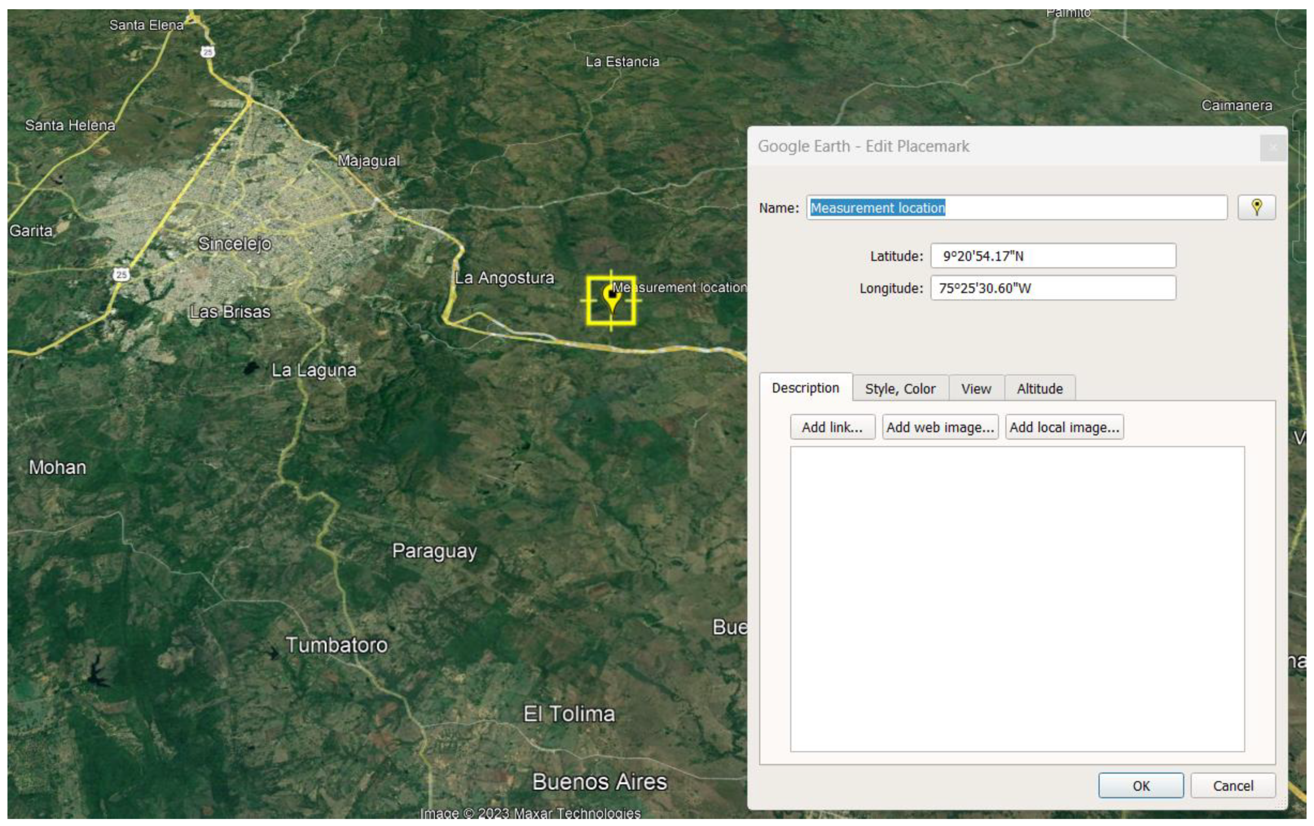
To analyze the propagation characteristics of the wireless channel, RSSI data were collected in a bitter cassava crop, which is mainly used as a raw material for starch production. The measurements were taken on a farm in the rural area of Sincelejo, capital of the department of Sucre, one of the largest producers in Colombia. The measurements were conducted on sunny days during the second planting period (August to March) at coordinates 9°2″53″ N latitude and 75°25″33″ W longitude (see Figure 1).

The cassava bushes were planted in a commonly used arrangement for this type of crop, with 120 cm between rows and 93 cm between plants. Figure 2 depicts the positioning of bushes in the selected cultivation. The measurement campaign was carried out using Digi Xbee XK3-Z8S-WZM transceiver modules operating on the IEEE 802.15.4 standard, capable of functioning as both Tx and Rx in the 2400 MHz band. The antennas at both ends are omnidirectional, which are commonly used in WSN deployments in agricultural environments [8]. The system parameters are presented in

Table 1. System parameters.

Parameter	Value
Frequency	2400 MHz
Antenna gain	2.1 dBi
Transmission power	8 dBm
Receiver sensitivity	−103 dBm
Antenna type	Omnidirectional

.

Data were collected and stored during three stages of bush growth. In each round, the Tx and Rx antennas were adjusted to heights of 80 cm, 130 cm, and 180 cm, with no obstructions other than the crop itself. The transmitting antenna was positioned at a fixed point, and the receiver was moved in 5 m increments, with equal antenna heights at each step. At each measurement point, 20 RSSI values were obtained and averaged, and additionally, tests were conducted with the transmission of 100 packets at intervals of 1000 ms. Because the spaces between rows of plants are commonly used as pathways by the individuals responsible for the plantation, the nodes were positioned along the rows of bushes. The receiver was moved until it reached the maximum distance between the rows of the crop, which in this case was 50 m, or until packet losses were recorded. The information obtained was stored on a computer connected to the transmitter module via USB. Figure 3a,b show a diagram of the applied set-up and the arrangement of the equipment in the culture.

Since the geographical area where the measurements were taken has limited mobile phone coverage by the operators providing service in the region, it was decided not to upload the data to any cloud platform. Instead, the data were backed up and isolated on an external memory stick, thus ensuring data protection.

2.3. Machine Learning Techniques

In machine learning, there are mainly two learning methods: supervised and unsupervised. The former requires initial data to detect patterns, while the latter learns the variable space without the use of labeled data [35]. In this research, we calculate the radio signal loss between a transmitter and a receiver in a cassava crop using a supervised approach with techniques that determine the attenuation from a set of measurements with varying values of distance, plant height, and antenna height.

One of the simplest and most widely used methods in supervised learning is linear regression (LR), where the prediction is made from the weighted sum of the input features and a constant called the intercept, as shown in Equation (5).

$$y={\beta }_0+{\beta }_1{x}_1+{\beta }_2{x}_2+\dots +{\beta }_n{x}_n,$$

(5)

where $y$ is the variable to predict, ${\beta }_i$ are the model parameters, $x_i$ is the i-th value of the features, and n is the number of features. The goal when training an LR model in ML is to find a value beta that minimizes the error [36]. Another advantage of LR is that models using this technique are less likely to overfit the data. However, as a drawback, it exhibits high sensitivity to outliers.

Support vector machine (SVM) is another regression technique widely used in ML but more advanced than LR. In SVM, the goal is to fit a hyperplane in a high-dimensional space that maximizes the distance to the nearest training data points of any class [37]. The hyperplane in the feature space can be described as the linear function shown in Equation (6) [38].

$$f\left(x\right)=w^{T}x+b,$$

(6)

where w corresponds to the vector determining the direction of the hyperplane, x is the input feature vector, and b is the bias term. The prediction function is presented in Equation (7).

$$f\left(x\right)=\sum _{i=1}^N\left(a_i-a_i^{*}\right)K\left(x_i, x\right)+b,$$

(7)

where $a_i$ and $a_i^{\mathrm{*}}$ are the Lagrange multipliers, $K$ represents the kernel used in the mapping, and i represents the sample number. Unlike other regression techniques, SVM is less sensitive to outliers in the data [39] but is dependent on the kernel used and data scaling [38]. Due to its advantages and effectiveness, SVM is a supervised learning technique successfully used in predicting path loss in various scenarios [40].

K-nearest neighbors (K-NN) is a technique that can be used in both regression and classification problems. It makes predictions on test vectors based on the learning obtained from training vectors [41]. K-NN uses distance functions as metrics to calculate the mean of the numerical target of the k-nearest neighbors. Equations (8)–(10) show the distance functions used in K-NN [42].

$$Euclidean: D=\sqrt{\sum _{i=1}^k{\left(x_i-y_i\right)}^2,}$$

(8)

$$Manhattan: D=\sum _{}^{}\left|x_i-y_i\right|,$$

(9)

$$Minkowski: D={\left(\sqrt{\sum _{i=1}^k{\left(\left|x_i-y_i\right|\right)}^q}\right)}^{\raisebox{1ex}{$1$}\!\left/ \!\raisebox{-1ex}{$q$}\right.}, q\ge 1,$$

(10)

where x is the measured value, and y is the predicted value. Although K-NN is a method that can yield good results when fitting the data, the computational effort increases as the size of the data used grows [42].

The fourth technique considered in this research is random forest (RF). It is a nonparametric approach used in regression and classification tasks and was developed as an improvement over decision trees [43]. Instead of using a single tree, random forest (RF) creates a ‘forest’ of random trees, each trained on a random sample of the data and a random selection of features. The predictions from all the trees are used to generate a final prediction [40,44]. Each new prediction at a point x with RF is obtained by taking the mean value of the predictions of each tree, ${\widehat{f}}_1$ … ${\widehat{f}}_{N_{Tree}}$, as shown in Equation (11) [45].

$${\widehat{f}}_{RF}\left(x\right)=\frac{1}{N_{Tree}}\sum _{\begin{array}{c}K=1\\ \end{array}}^{N_{Tree}}{\widehat{f}}_K\left(x\right),$$

(11)

These techniques, along with others in the field of ML, can be considered valid alternatives when modeling radio wave propagation in different scenarios. However, since no validation method allows the best one to be selected in advance, it is common practice to try different algorithms to see which one performs better for a given problem [41]. Therefore, due to the amount of data and variables used in the training process, as well as the ease of implementation, interpretation, and computational efficiency, the following algorithms have been chosen for this research: LR, SVM, K-NN, and RF.

3. Results

3.1. Comparison of Models

We evaluated the effectiveness of the vegetative models presented in Section 2.1 by comparing them with results obtained from the measurement campaign. Since it is preferable to monitor the crop from the beginning of the planting process, measurements were taken at three different stages of average plant growth (50 cm, 150 cm, and 190 cm). The obtained RSSI values indicate that the radio signal range was greater when the antennas were configured at heights of 180 cm for plant sizes of 50 cm and 150 cm, as they exhibited line-of-sight (LoS) conditions. However, during the stage of maximum bush growth and with the same configuration of experimental conditions applied in the first two measurement stages, the best coverage was achieved with antennas placed 80 cm above ground level. The path loss was calculated from the RSSI measurements at each measurement point using Equation (12).

$$PL\left(dB\right)=P_{Tx}+G_{Tx}+G_{Rx}-P_{Rx},$$

(12)

where P_Tx is the transmission power, G_Tx and G_Rx are the gains of the transmitter and receiver antennas, respectively, and P_Rx is the received power at the receiver determined from the RSSI. Since the vegetative models only consider the loss caused by foliage and not the total loss along the link, the analysis was complemented with the free space path loss (FSPL) model to calculate the total attenuation along the path [46,47]. Figure 4a–c depict the behavior of the measured losses concerning the measurement distance in each of the three stages of cultivation where measurements were taken, along with the estimations obtained using the vegetative models.

Additionally, the root mean square error (RMSE) was calculated, which is one of the most used tools for evaluating the effectiveness of radio wave propagation models. This is presented in Equation (13).

$$RMSE=\sqrt{\frac{1}{N}\times \sum _{i=1}^N{\left(x_i-{\widehat{x}}_i\right)}^2,}$$

(13)

where $x_i$ and ${\widehat{x}}_i$ are the measured and predicted values, respectively, and N corresponds to the number of samples. In this case, the higher the RMSE value, the lower the ability of the models to accurately predict actual crop losses.

Figure 4a–c, along with the obtained RMSE, indicate that in all measurement stages and for each antenna height configuration, the FSPL+FITU-R combination underestimated the measurements, reaching minimum RMSE values of 19.99 and maximum values of 29.86. For FSPL+ITU-R, it underestimated the losses in stages 1 and 3, but the RMSE decreased to values of 8.72 and 19.05, respectively. Meanwhile, in stage 2, it overestimated the measurements when the antennas were placed at 80 cm and 130 cm above the ground and underestimated them at 190 cm, giving an RMSE of 15.21. Finally, FSPL+COST-235 exhibited the best performance in stages 1 and 3, achieving the lowest error values in estimating the losses. It showed a trend of losses with values higher than the measurements and RMSE of 6.81 and 6.39, respectively. However, in stage 2, the estimation error increased, reaching a value of 17.4. These results show that the propagation and the range of the modules are affected by the modifications of the different experimental conditions that have been proposed. Furthermore, the vegetative models considered in this study do not estimate cassava crop losses with error levels considered acceptable. Therefore, it is necessary to adjust or develop a model for this specific environment.

3.2. New Model

In this study, we calculated the loss of radio signals between a transmitter and a receiver in a cassava crop using a supervised approach with algorithms that determine attenuation based on a series of measurements at different distances, plant heights, and antenna heights. The correlation matrix with the contribution of each attribute considered in the study is shown in Figure 5. It is observed that losses in cassava crops are highly affected by clearing losses (considering frequency and distance), followed by cassava bush height and antenna height.

In the proposed methodology, we selected 70% of the dataset for training and 30% for testing, applying this procedure with the evaluated techniques LR, K-NN, SVM, and RF. In the case of K-NN, the used kernel was optimal with k-neighbors equal to 16, while in SVM, the implemented kernel is a radial basis function, with data scaling. Regarding RF, we adjusted the number of trees to 20. Taking into account the evaluation metrics used in similar studies [38,48,49,50], in this work, we have considered the RMSE presented in Section 3, as well as the mean absolute error (MAE) and the coefficient of determination (referred to as R²), calculated using Equations (14) and (15), respectively.

$$MAE=\frac{1}{n}\sum _{i=1}^n{x}_i-{\widehat{x}}_i,$$

(14)

$$R^2=\frac{{\sum }_{i=1}^n{\left(x_i-\overline{x}\right)}^2}{{\sum }_{i=1}^n{\left({\widehat{x}}_i-\overline{x}\right)}^2},$$

(15)

where $x_i$, $\overline{x,}$ and ${\widehat{x}}_i$ are the measured values, mean of the values, and predicted values, respectively. Additionally, n represents the number of samples. In the case of RMSE and MAE, the models exhibit a better fit of the data as they tend toward zero, while in the case of R², it indicates that it is capable of accurately representing the data as it tends toward 1.

The performance of the models obtained from the use of LR, K-NN, SVM, and RF with the training and testing dataset is presented in

Table 2. Performance comparison of ML models.

Model	RMSE	MAE	R2
LR	8.81	7.29	0.4650
K-NN	2.62	1.76	0.9575
SVM	2.66	1.85	0.9507
RF	2.51	1.78	0.9604

. The results of the metrics indicate that the models obtained from RF, K-NN, and SVM predict path losses in the studied crop with low levels of error, significantly outperforming the vegetative models UIT-R, FITU-R, and COST-235. However, when using LR as an algorithm in ML, the error values increase considerably, making it the technique with the poorest performance.

Further analysis of the results reveals that RF offers the best performance (RMSE = 2.51, MAE = 1.78, and R² = 0.9604). The evaluation metrics demonstrate that K-NN can perform regression based on the training data, with minimal variation compared to the results obtained with RF. As for the SVM using the radial basis function, it is evident that it is also capable of accurate path loss predictions in the study scenario, keeping the RMSE and MAE values below 5 dB and an R² slightly above 95%. 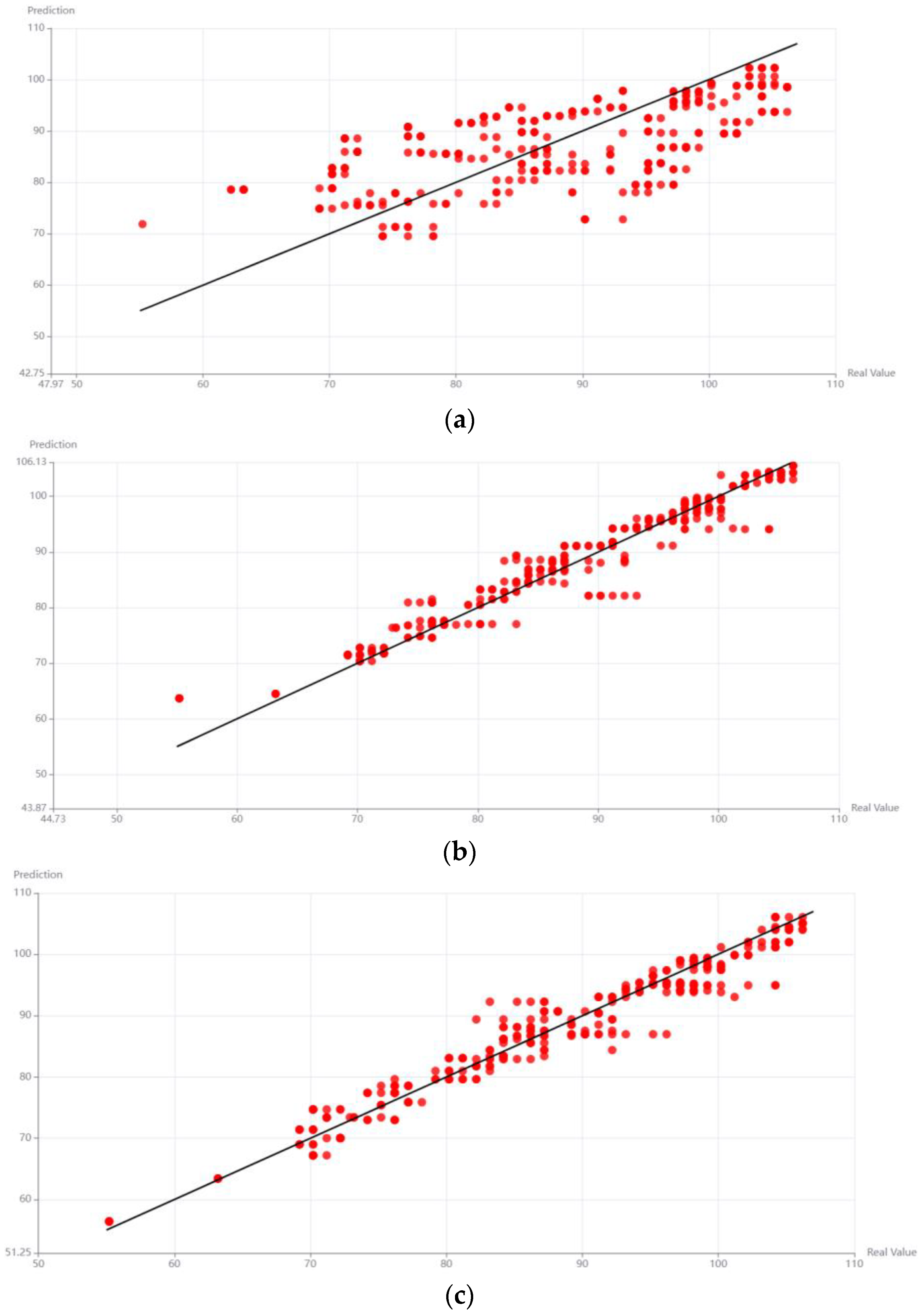In addition, Figure 6a–d show the scatter plots of the values, showing the difference between the expected prediction and the results obtained with the models. Black lines represent ideal predictions for each model, while red dots represent predicted path loss values. In the case of LR, the predictor exhibits a negative bias when the path loss values exceed 94 dB and a positive bias around 85 dB. Regarding K-NN, SVM, and RF, it demonstrates a bias very close to zero but becomes positive for path loss values around 88 dB.

Although the evaluation metrics indicate that RF gives better results than SVM, they are not significantly different. However, since SVM has proven to be a superior method compared to other supervised learning techniques [47], it could be considered a preferable alternative in the modeling of WSN systems in crops, as it is less computationally demanding than RF. Regarding LR, it is a simple method that generally yields good results. Nevertheless, in this study, it turned out to be the least performing one with RMSE or MAE values too high, and given the goodness of fit below 70%, its application in modeling path losses in the studied crop is not considered useful.

4. Discussion

In this paper, we compare three vegetative propagation models (ITU-R, FITU-R, and COST-235) with path loss data from a cassava crop. For this purpose, we carried out measurements at three stages of crop growth and under different conditions of distance and height of the transmitting and receiving antennas. The results demonstrate that none of the considered vegetative models could estimate the losses with an acceptable level of error. On the contrary, the RMSE values were above 10 dB in most of the experimental conditions.

Furthermore, in this study, we departed from the traditional approach of modeling losses from a physics perspective. On the contrary, we have embraced a more contemporary orientation based on machine learning (ML) by employing LR, K-NN SVM, and RF techniques within a training–testing method. From this approach, loss prediction is substantially improved. The use of RF, K-NN, and SVM allowed for a reduction in errors, achieving RMSE values below 3 dB and MAE values below 2 dB. Furthermore, the R² results obtained demonstrate that ML models can characterize losses with a high level of accuracy. However, it is important to note that not all ML techniques applied were successful, as LR did not yield satisfactory evaluation metrics (RMSE = 8.81, MAE = 7.29, and R² = 0.4650). Despite the favorable outcomes, it is crucial to consider additional factors when selecting an ML technique to predict path losses in cassava crops—for instance, the volume of data, computational requirements, and the performance of predictions across the entire range of experimental choices.

5. Conclusions

Though the results achieved through ML usage are satisfactory, it is important to emphasize the study’s limitations, particularly the omission of additional factors that significantly influence radio signal attenuation. For instance, our experimentation was conducted in the 2400 MHz band and was not extended to other frequencies. Another factor to consider is that changes in environmental conditions (such as bushes of different varieties or changes in the arrangement of plants in the crop) can significantly affect the results, which is inherent in empirical propagation models.

Despite its advantages, ML does not define the variables that should be used in model generation; these are left to the researchers’ discretion. Furthermore, there is no standardized methodology that outlines the conditions for data collection and model development. Therefore, a profound understanding of propagation matters, and the conditions under which measurements should be conducted remains essential, ensuring the proper correlation between the study’s aspects and the acquired data.

To extend the results, it is recommended that future work extends the dataset. An alternative is to expand measurements throughout the entire process of bush growth. In addition, experiments should be carried out in other ISM frequency bands commonly used for WSN deployment (e.g., the 900 MHz band). It would be equally relevant to consider variables related to the shrub, such as stem thickness and leaf dimensions, as well as climatic factors, such as rainfall and humidity. The study could also be extended by analyzing data from other crops considered important for food sustainability, such as maize, rice, potatoes, or fruits. Future studies could also involve mixed crop or foliage scenarios in rural environments, such as gardens or parks.

For future work, they might consider using other ML techniques, such as lasso regression or neural networks, so that their results help to improve the analysis. Other regression techniques, such as quadratic or cubic regression, could also be further evaluated to see if they improve levels of fit and decrease error metrics. Furthermore, it is feasible to extend the study to other crops of importance for food sustainability, such as rice or potatoes. Furthermore, future research should address strengthening the security of the data collected during the measurement process to preserve their integrity and reduce vulnerability to potential cyberattacks.

References

- Beckman, J.; Countryman, A.M. The Importance of Agriculture in the Economy: Impacts from COVID-19. Am. J. Agric. Econ. 2021, 103, 1595–1611. [Google Scholar] [CrossRef] [PubMed]
- Arrubla-Hoyos, W.; Ojeda-Beltrán, A.; Solano-Barliza, A.; Rambauth-Ibarra, G.; Barrios-Ulloa, A.; Cama-Pinto, D.; Arrabal-Campos, F.M.; Martínez-Lao, J.A.; Cama-Pinto, A.; Manzano-Agugliaro, F. Precision Agriculture and Sensor Systems Applications in Colombia through 5G Networks. Sensors 2022, 22, 7295. [Google Scholar] [CrossRef] [PubMed]
- International Society of Precision Agriculture Precision AG Definition. Available online: https://www.ispag.org/about/definition (accessed on 3 April 2023).
- Zhang, C.; Lu, Y. Study on artificial intelligence: The state of the art and future prospects. J. Ind. Inf. Integr. 2021, 23, 100224. [Google Scholar] [CrossRef]
- Barrios-Ulloa, A.; Ariza-Colpas, P.P.; Sánchez-Moreno, H.; Quintero-Linero, A.P.; De la Hoz-Franco, E. Modeling Radio Wave Propagation for Wireless Sensor Networks in Vegetated Environments: A Systematic Literature Review. Sensors 2022, 22, 5285. [Google Scholar] [CrossRef]
- Sander-Frigau, M.; Zhang, T.; Lim, C.Y.; Zhang, H.; Kamal, A.E.; Somani, A.K.; Hey, S.; Schnable, P. A Measurement Study of TVWS Wireless Channels in Crop Farms. In Proceedings of the 2021 IEEE 18th International Conference on Mobile Ad Hoc and Smart Systems (MASS), Denver, CO, USA, 4–7 October 2021; pp. 344–354. [Google Scholar] [CrossRef]
- Pal, P.; Sharma, R.P.; Tripathi, S.; Kumar, C.; Ramesh, D. 2.4 GHz RF Received Signal Strength Based Node Separation in WSN Monitoring Infrastructure for Millet and Rice Vegetation. IEEE Sens. J. 2021, 21, 18298–18306. [Google Scholar] [CrossRef]
- Cama-Pinto, D.; Damas, M.; Holgado-Terriza, J.A.; Gómez-Mula, F.; Cama-Pinto, A. Path loss determination using linear and cubic regression inside a classic tomato greenhouse. Int. J. Environ. Res. Public Health 2019, 16, 1744. [Google Scholar] [CrossRef]
- Ganev, Z. Log-normal shadowing model for outdoor propagation between sensor nodes. In Proceedings of the 2018 20th International Symposium on Electrical Apparatus and Technologies (SIELA), Bourgas, Bulgaria, 3–6 June 2018; pp. 9–12. [Google Scholar]
- Miao, Y.; Zhao, C.; Wu, H. Non-uniform clustering routing protocol of wheat farmland based on effective energy consumption. Int. J. Agric. Biol. Eng. 2021, 14, 163–170. [Google Scholar] [CrossRef]
- Navarro, A.; Guevara, D.; Florez, G.A. An Adjusted Propagation Model for Wireless Sensor Networks in Corn Fields. In Proceedings of the 020 XXXIIIrd General Assembly and Scientific Symposium of the International Union of Radio Science, Rome, Italy, 29 August–5 September 2020; pp. 1–3. [Google Scholar]
- FAO. Save and Grow: Cassava a Guide to Sustainable Production Intensification. Available online: https://www.fao.org/publications/card/en/c/c3ef3b0e-492e-5ea8-816c-8d1e3b86d66b/ (accessed on 4 April 2023).
- OECD-FAO Agricultural Outlook 2020–2029. Available online: https://www.oecd-ilibrary.org/agriculture-and-food/oecd-fao-agricultural-outlook-2020-2029_1112c23b-en (accessed on 4 April 2023).
- Caicedo-Ortiz, J.G.; De-la-Hoz-Franco, E.; Morales Ortega, R.; Piñeres-Espitia, G.; Combita-Niño, H.; Estévez, F.; Cama-Pinto, A. Monitoring system for agronomic variables based in WSN technology on cassava crops. Comput. Electron. Agric. 2018, 145, 275–281. [Google Scholar] [CrossRef]
- Manick; Srivastava, J. Cassava Leaf Disease Detection Using Deep Learning. In Proceedings of the 2022 IEEE International IOT, Electronics and Mechatronics Conference (IEMTRONICS), Toronto, ON, Canada, 1–4 June 2022. [Google Scholar] [CrossRef]
- Maryum, A.; Akram, M.U.; Salam, A.A. Cassava Leaf Disease Classification using Deep Neural Networks. In Proceedings of the 2021 IEEE 18th International Conference on Smart Communities: Improving Quality of Life Using ICT, IoT and AI (HONET), Karachi, Pakistan, 11–13 October 2021; pp. 32–37. [Google Scholar] [CrossRef]
- Chen, C.C.; Ba, J.Y.; Li, T.J.; Chan, C.C.K.; Wang, K.C.; Liu, Z. EfficientNet: A low-bandwidth IoT image sensor framework for cassava leaf disease classification. Sens. Mater. 2021, 33, 4031–4044. [Google Scholar] [CrossRef]
- Gao, Z.; Li, W.; Zhu, Y.; Tian, Y.; Pang, F.; Cao, W.; Ni, J. Wireless channel propagation characteristics and modeling research in rice field sensor networks. Sensors 2018, 18, 3116. [Google Scholar] [CrossRef]
- Pal, P.; Sharma, R.P.; Tripathi, S.; Kumar, C.; Ramesh, D. Machine Learning Regression for RF Path Loss Estimation Over Grass Vegetation in IoWSN Monitoring Infrastructure. IEEE Trans. Ind. Inform. 2022, 18, 6981–6990. [Google Scholar] [CrossRef]
- Phokharatkul, P.; Phaiboon, S. Path Loss Model for the Bananas and Weeds Environment Based on Grey System Theory. In Proceedings of the 2021 Photonics & Electromagnetics Research Symposium (PIERS), Hangzhou, China, 21–25 November 2021; pp. 413–418. [Google Scholar] [CrossRef]
- Anzum, R.; Hadi Habaebi, M.; Islam, R.; Hakim, G.P.N. Modeling and Quantifying Palm Trees Foliage Loss using LoRa Radio Links for Smart Agriculture Applications. In Proceedings of the 2021 IEEE 7th International Conference on Smart Instrumentation, Measurement and Applications (ICSIMA), Bandung, Indonesia, 23–25 August 2021; pp. 105–110. [Google Scholar] [CrossRef]
- Juan-Llacer, L.; Molina-Garcia-Pardo, J.M.; Sibille, A.; Torrico, S.A.; Rubiola, L.M.; Martinez-Ingles, M.T.; Rodriguez, J.V.; Pascual-Garcia, J. Path Loss Measurements and Modelling in a Citrus Plantation in the 1800 MHz, 3.5 GHz and 28 GHz in LoS. In Proceedings of the 2022 16th European Conference on Antennas and Propagation (EuCAP), Madrid, Spain, 27 March–1 April 2022. [Google Scholar] [CrossRef]
- Wu, H.; Zhu, H.; Han, X.; Xu, W. Layout optimization for greenhouse WSN based on path loss analysis. Comput. Syst. Sci. Eng. 2021, 37, 89–104. [Google Scholar] [CrossRef]
- Kale, A.; Nguyen, T.; Harris, F.C.; Li, C.; Zhang, J.; Ma, X. Provenance documentation to enable explainable and trustworthy AI: A literature review. Data Intell. 2023, 5, 139–162. [Google Scholar] [CrossRef]
- Oroza, C.A.; Zhang, Z.; Watteyne, T.; Glaser, S.D. A Machine-Learning-Based Connectivity Model for Complex Terrain Large-Scale Low-Power Wireless Deployments. IEEE Trans. Cogn. Commun. Netw. 2017, 3, 576–584. [Google Scholar] [CrossRef]
- Kochhar, A.; Kumar, N.; Arora, U. Signal Assessment Using ML for Evaluation of WSN Framework in greenhouse monitoring. Int. J. Sensors Wirel. Commun. Control 2022, 12, 669–679. [Google Scholar] [CrossRef]
- ITU-R. ITU-R Recommendation P.833-7 Attenuation in Vegetation; ITU-R: Geneva, Switzerland, 2012; Volume 7. [Google Scholar]
- Olasupo, T.O.; Otero, C.E. The Impacts of Node Orientation on Radio Propagation Models for Airborne-Deployed Sensor Networks in Large-Scale Tree Vegetation Terrains. IEEE Trans. Syst. Man Cybern. Syst. 2020, 50, 256–269. [Google Scholar] [CrossRef]
- Sabri, N.; Mohammed, S.S.; Fouad, S.; Syed, A.A.; Al-Dhief, F.T.; Raheemah, A. Investigation of Empirical Wave Propagation Models in Precision Agriculture. MATEC Web Conf. 2018, 150, 06020. [Google Scholar] [CrossRef]
- Raheemah, A.; Sabri, N.; Salim, M.S.; Ehkan, P.; Ahmad, R.B. New empirical path loss model for wireless sensor networks in mango greenhouses. Comput. Electron. Agric. 2016, 127, 553–560. [Google Scholar] [CrossRef]
- Anzum, R.; Habaebi, M.H.; Islam, M.R.; Hakim, G.P.N.; Khandaker, M.U.; Osman, H.; Alamri, S.; AbdElrahim, E. A Multiwall Path-Loss Prediction Model Using 433 MHz LoRa-WAN Frequency to Characterize Foliage’s Influence in a Malaysian Palm Oil Plantation Environment. Sensors 2022, 22, 5397. [Google Scholar] [CrossRef]
- Dogan, H. A new empirical propagation model depending on volumetric density in citrus orchards for wireless sensor network applications at sub-6 GHz frequency region. Int. J. RF Microw. Comput. Eng. 2021, 31, e22778. [Google Scholar] [CrossRef]
- Shaik, M.; Kabanni, A.; Nazeema, N. Millimeter wave propagation measurments in forest for 5G Wireless sensor communications. In Proceedings of the 2016 16th Mediterranean Microwave Symposium (MMS), Abu Dhabi, United Arab Emirates, 14–16 November 2016; pp. 1–4. [Google Scholar] [CrossRef]
- Olasupo, T.O.; Alsayyari, A.; Otero, C.E.; Olasupo, K.O.; Kostanic, I. Empirical path loss models for low power wireless sensor nodes deployed on the ground in different terrains. In Proceedings of the 2017 IEEE Jordan Conference on Applied Electrical Engineering and Computing Technologies (AEECT), Aqaba, Jordan, 11–13 October 2017; pp. 1–8. [Google Scholar]
- Burkov, A. The Hundred-Page Machine Learning; Burkov, A., Ed.; Andriy Burkov: Quebec City, QC, Canada, 2019; ISBN 978-1-9995795-1-7. [Google Scholar]
- Géron, A. Hands-on Machine Learning with Scikit-Learn, Keras, and TensorFlow, 2nd ed.; Tache, N., Ed.; O’Reilly Media: Sebastopol, CA, USA, 2019; ISBN 1098125975. [Google Scholar]
- Zhang, J.; Liu, L.; Fan, Y.; Zhuang, L.; Zhou, T.; Piao, Z. Wireless Channel Propagation Scenarios Identification: A Perspective of Machine Learning. IEEE Access 2020, 8, 47797–47806. [Google Scholar] [CrossRef]
- Zhang, Y.; Wen, J.; Yang, G.; He, Z.; Wang, J. Path loss prediction based on machine learning: Principle, method, and data expansion. Appl. Sci. 2019, 9, 1908. [Google Scholar] [CrossRef]
- Theobald, O. Machine Learning for Absolute Beginners; Independently published, 2017; ISBN 978-1520951409.
- Moraitis, N.; Tsipi, L.; Vouyioukas, D.; Gkioni, A.; Louvros, S. Performance evaluation of machine learning methods for path loss prediction in rural environment at 3.7 GHz. Wirel. Netw. 2021, 27, 4169–4188. [Google Scholar] [CrossRef]
- Vergos, G.; Sotiroudis, S.P.; Athanasiadou, G.; Tsoulos, G.V.; Goudos, S.K. Comparing Machine Learning Methods for Air-to-Ground Path Loss Prediction. In Proceedings of the 2021 10th International Conference on Modern Circuits and Systems Technologies, MOCAST, Thessaloniki, Greece, 5–7 July 2021; pp. 1–4. [Google Scholar]
- Elmezughi, M.K.; Salih, O.; Afullo, T.J.; Duffy, K.J. Comparative Analysis of Major Machine-Learning-Based Path Loss Models for Enclosed Indoor Channels. Sensors 2022, 22, 4967. [Google Scholar] [CrossRef] [PubMed]
- Breiman, L. Random Forest. Mach Learn 2001, 45, 5–32. [Google Scholar] [CrossRef]
- Probst, P.; Wright, M.N.; Boulesteix, A.L. Hyperparameters and tuning strategies for random forest. Wiley Interdiscip. Rev. Data Min. Knowl. Discov. 2019, 9, e1301. [Google Scholar] [CrossRef]
- Antoniadis, A.; Lambert-Lacroix, S.; Poggi, J.-M. Random forests for global sensitivity analysis: A selective review. Reliab. Eng. Syst. Safe 2021, 206, 107312. [Google Scholar] [CrossRef]
- Cama-Pinto, D.; Damas, M.; Holgado-Terriza, J.A.; Arrabal-Campos, F.M.; Gómez-Mula, F.; Lao, J.A.M.; Cama-Pinto, A. Empirical model of radio wave propagation in the presence of vegetation inside greenhouses using regularized regressions. Sensors 2020, 20, 6621. [Google Scholar] [CrossRef]
- Vougioukas, S.; Anastassiu, H.T.; Regen, C.; Zude, M. Influence of foliage on radio path losses (PLs) for Wireless Sensor Network (WSN) planning in orchards. Biosyst. Eng. 2013, 114, 454–465. [Google Scholar] [CrossRef]
- Nagao, T.; Hayashi, T. Fine-Tuning for Propagation Modeling of Different Frequencies with Few Data. In Proceedings of the 2022 IEEE 96th Vehicular Technology Conference (VTC2022-Fall), London, UK, 26–29 September 2022; pp. 1–5. [Google Scholar] [CrossRef]
- Goudos, S.K.; Athanasiadou, G.; Tsoulos, G.V.; Rekkas, V. Modelling Ray Tracing Propagation Data Using Different Machine Learning Algorithms. In Proceedings of the 2020 14th European Conference on Antennas and Propagation (EuCAP), Copenhagen, Denmark, 15–20 March 2020. [Google Scholar]
- Jo, H.S.; Park, C.; Lee, E.; Choi, H.K.; Park, J. Path loss prediction based on machine learning techniques: Principal component analysis, artificial neural network and gaussian process. Sensors 2020, 20, 1927. [Google Scholar] [CrossRef]