Estimation of Error Variance in Genomic Selection for Ultrahigh Dimensional Data

Abstract

Estimation of error variance in the case of genomic selection is a necessary step to measure the accuracy of the genomic selection model. For genomic selection, whole-genome high-density marker data is used where the number of markers is always larger than the sample size. This makes it difficult to estimate the error variance because the ordinary least square estimation technique cannot be used in the case of datasets where the number of parameters is greater than the number of individuals (i.e., p > n). In this article, two existing methods, viz. Refitted Cross Validation (RCV) and kfold-RCV, were suggested for such cases. Moreover, by considering the limitations of the above methods, two new methods, viz. Bootstrap-RCV and Ensemble method, have been proposed. Furthermore, an R package “varEst” has been developed, which contains four different functions to implement these error variance estimation methods in the case of Least Absolute Shrinkage and Selection Operator (LASSO), Least Squares Regression (LSR) and Sparse Additive Models (SpAM). The performances of the algorithms have been evaluated using simulated and real datasets.

1. Introduction

Genomic Selection (GS) is an advanced form of marker-assisted selection used in the breeding of animals and plants. GS was first described by Meuwissen et al. in 2001 [1]. GS increases genetic gain by reducing the duration of the breeding cycle. Moreover, in GS, there is no need to have information about the exact location of the associated gene. Markers from the whole genome are used in GS to estimate the breeding value, which is known as Genomic Estimated Breeding Value (GEBV), used for the selection of individuals. So, GS deals with millions of markers all over the genome, and this leads to a statistical issue known as p > n problem, where p is the number of variables (markers) and n is the sample size (number of individuals).

There are several statistical models available to estimate the GEBV in the case of GS. However, the performance of these models needs to be evaluated properly. For that, we need to estimate the error variance of each model. However, error variance estimation is a difficult problem in additive models when p > n. Standard least squares estimation techniques cannot be applied in this case. Poor estimation of error variance of a genomic selection model also leads to poor estimation of the GEBV in GS. In order to resolve this problem, several variance estimators have been proposed but mostly all suffer large biases in finite samples. Fan et al. proposed the Refitted Cross Validation (RCV) method in 2012 to overcome the downward bias of the Least Absolute Shrinkage and Selection Operator (LASSO) estimator for the estimation of error variance [2]. They have also mentioned a modification of the RCV method called k-fold RCV where the dataset is divided into k numbers of subgroups instead of two groups as in the case of RCV. Other error variance estimation methods include the oracle estimator, residual sum of squares-based estimators [2], cross-validation based estimators [2], Smoothly Clipped Absolute Deviation Penalty (SCAD) estimator [3], scaled sparse linear regression estimators [4] and method of moments estimators [5]. Chen et al. (2018) have proposed an estimator for error variance in an ultrahigh dimensional sparse additive model by effectively integrating sure independence screening and Refitted Cross Validation techniques [6]. Yu and Bien have proposed the natural LASSO estimator and organic LASSO estimator for the error variance estimation in the high dimensional linear model [7]. A ridge regression and random matrix theory-based novel estimator of error variance has been proposed by Liu et al. [8]. A residual-based efficient estimator for error variance has been developed by Li et al., 2020 [9].

However, hardly any review is available related to the application of these methods in variance estimation for genomic selection. In this article, it is probably the first time we have used the algorithm of RCV method and k-fold RCV method proposed by Fan et al. in 2012 in genomic selection for variance estimation. Moreover, we have extended the work done by Fan et al. and developed a new algorithm for variance estimation called “bootstrap RCV”. It has been observed that sometimes particularly in big data, such as genotypic data, RCV method suffers from a computational problem. In order to resolve this problem, we have developed a new computationally efficient algorithm based on the Ensemble approach. Performances of these algorithms have been tested using simulated data for different genetic architectures (different heritability and epistasis level). All these algorithms are implemented in R to develop an R package “varEst” [10] for estimating the error variance of Genomic Selection models.

2. Materials and Methods

2.1. Simulated Dataset

For this study, 24 genomic datasets, including both genotype and phenotype data, were simulated. There were 10 true features known as Quantitative Trait Loci (QTLs) in the datasets. An R package QTL Bayesian interval mapping (“qtlbim”) [11,12] was used to simulate the genome with 10 chromosomes. The package qtlbim follows Cockerham’s model for simulating quantitative trait loci with epistasis [13]. The Cockerham’s model for quantitative trait controlled by two epistatic genes A and B, from a sample of size n of an F2 population, the trait value of the $k$th individual with genotype $ij$ can be described as follows:

$$y_{ijk}=G_{ij}+{\epsilon }_{ijk}=\mu +a_1{x}_1+d_1{z}_1+a_2{x}_2+d_2{z}_2+i_{aa}{w}_{aa}+i_{ad}{w}_{ad}+i_{da}{w}_{da}+i_{dd}{w}_{dd}+{\epsilon }_{ijk}$$

where $G_{ij}$ denotes the genotypic value of the genotype $ij$, $\mu$ is the mean, $a_1$ is the additive effect of locus A, $d_1$ is the dominance effect of locus A, $a_2$ is the additive effect of locus B, $d_2$ is the dominance effect of locus B, $i_{aa}$ is additive × additive effect of loci A and B, $i_{ad}$ is additive × dominance effect of loci A and B, $i_{da}$ is dominance × additive effect of loci A and B, $i_{dd}$ is dominance × dominance effect of loci A and B. The coded variables are defined as

$$x_1=\{\begin{array}{c} 1 if A is AA\\ 0 if A is Aa\\ -1 if A is aa\end{array} x_2=\{\begin{array}{c} 1 if B is BB\\ 0 if B is Bb\\ -1 if B is bb\end{array}$$

$$z_1=\{\begin{array}{c}\raisebox{1ex}{$1$}\!\left/ \!\raisebox{-1ex}{$2$}\right. if A is Aa\\ -\raisebox{1ex}{$1$}\!\left/ \!\raisebox{-1ex}{$2$}\right. otherwise\end{array}{z}_2=\{\begin{array}{c}\raisebox{1ex}{$1$}\!\left/ \!\raisebox{-1ex}{$2$}\right. if B is Bb\\ -\raisebox{1ex}{$1$}\!\left/ \!\raisebox{-1ex}{$2$}\right. otherwise\end{array}$$

$$w_{aa}=x_1\times x_2 w_{ad}=x_1\times z_2 w_{da}=z_1\times x_2 w_{dd}=z_1\times z_2$$

and ${\epsilon }_{ijk}$ is residual of the $k$th individual with genotype $ij$.

The genome contains 1000 markers, equally spaced over the chromosomes, and each chromosome has 100 markers. The phenotypic values are normally distributed and generated on the basis of 10 QTLs (true features). There are two categories of datasets, one of which is additive in nature and does not contain any epistatic effect, and the other category contains both additive and epistatic effects. So, the additive datasets have 10 QTLs, one each in every chromosome, whereas non-additive datasets have one pair of QTLs in 5 of the 10 chromosomes, the rest of the 5 chromosomes do not contain any QTL. In this way, 24 different datasets with different genetic architecture (i.e., with different levels of narrow-sense heritability (0.1, 0.2, 0.3, 0.5, 0.7 and 0.9) and epistatic effects, i.e., additive × additive effect (0, 5, 10 and 15)) are generated with genotypic and phenotypic information for F2 population. Each dataset contains 200 individuals and 1000 biallelic markers. A total of 500 replicates were simulated for each genetic architecture to predict phenotype (GEBV).

2.2. Real Dataset

We have two real datasets for this study, one is for wheat, and another is maize data [14]. Wheat lines were genotyped by Triticarte Pty. Ltd. (Canberra, Australia) using 1447 Diversity Array Technology. This data set includes 599 lines observed for trait grain yield (GY) for four mega environments. However, for our convenience, we have just considered GY for the first mega environment. The final number of DArT markers after editing was 1279; hence the same has been used in this study. The second dataset, which is the maize dataset, is generated by CIMMYT’s Global Maize Program. It originally included 300 maize lines with 1148 SNP markers. Here also, the trait under study is GY, evaluated under drought and watered conditions. After some editing, 264 maize lines with 1135 SNPs markers were available for the final study. The editing was done to improve the quality of the data by removing missing genotypes and outliers.

2.3. Methods for Error Variance Estimation

In this section, details of the algorithm for Refitted Cross Validation (RCV) and k-fold Refitted Cross Validation (k-RCV) method of error variance estimation in genomic selection are described.

2.3.1. Refitted Cross Validation (RCV)

The Refitted Cross Validation method is originally given by Fan et al. in 2012 for error variance estimation in ultrahigh dimensional regression [2]. A sample of size n is assumed and split randomly into two groups. In the first stage, the most relevant variables were selected with the help of an ultrahigh dimensional variable selection method from those two datasets separately. This step results in two small sets of important variables (markers). Here, in this study, we have applied SpAM [15], LASSO [16] and Linear Least Squares Regression as feature selection methods. The second stage involves the re-estimation of the regression coefficient β and variance σ² with the help of the ordinary least squares regression method. For this purpose, the variables selected from the first dataset are considered to estimate the variance from the second dataset and vice-versa. Finally, the average of those two variances, which we get from the second stage, is considered the final estimator of σ² (Figure 1). So, in the second stage, refitting is done to reduce the effect of spurious variables in the datasets, and also it takes care of the p > n problem in the high dimensional genomic datasets. The algorithm of the RCV method has been described below:

• Consider a dataset $\left(X_{n\times p},Y_{n\times 1}\right)$. We denote it as $S$;
• $S$ is divided into two groups randomly, each subsample having size of n/2;

  $$S=\left\{S^{\left(1\right)},S^{\left(2\right)}\right\}$$

  where $S^{\left(1\right)}=\left(X_{\left(n/2\right)\times p}^{\left(1\right)},Y_{\left(n/2\right)\times 1}^{\left(1\right)}\right)$ and $S^{\left(2\right)}=\left(X_{\left(n/2\right)\times p}^{\left(2\right)},Y_{\left(n/2\right)\times 1}^{\left(2\right)}\right)$.
• Variable selection has been performed on $S^{\left(1\right)}$ using SpAM or LASSO or Least Squares Regression and let $M^{\left(1\right)}$ is a set of selected variables from subsample $S^{\left(1\right)}$;
• Using only the selected variables i.e., $M^{\left(1\right)}$, error variance is estimated through $S^{\left(2\right)}$ with ordinary least squares estimation;

  $${{\widehat{\sigma }}^{\left(2\right)}}^2=\frac{Y^{{\left(2\right)}^T}\left(I_{\frac{n}{2}}-P_{M^{\left(1\right)}}^{\left(2\right)}\right)Y^{\left(2\right)}}{\frac{n}{2}-\left|M^{\left(1\right)}\right|}$$

  where $P_{M^{\left(1\right)}}^{\left(2\right)}=X_{M^{\left(1\right)}}^{\left(2\right)}{\left(X_{M^{\left(1\right)}}^{\left(2\right)}{}^T{X}_{M^{\left(1\right)}}^{\left(2\right)}\right)}^{-1}{X}_{M^{\left(1\right)}}^{\left(2\right)}{}^T$.
• In the next stage, variable selection has been performed on $S^{\left(2\right)}$ using Sparse Additive Models (SpAM) or LASSO or Least Squares Regression and $M^{\left(2\right)}$ is a set of selected variables from subsample $S^{\left(2\right)}$;
• Using only the selected variables i.e., $M^{\left(2\right)}$, variance is estimated in $S^{\left(1\right)}$ with ordinary least squares estimation;

  $${{\widehat{\sigma }}^{\left(1\right)}}^2=\frac{Y^{{\left(1\right)}^T}\left(I_{\frac{n}{2}}-P_{M^{\left(2\right)}}^{\left(1\right)}\right)Y^{\left(1\right)}}{\frac{n}{2}-\left|M^{\left(2\right)}\right|}$$

  where $P_{M^{\left(2\right)}}^{\left(1\right)}=X_{M^{\left(2\right)}}^{\left(1\right)}{\left({X_{M^{\left(2\right)}}^{\left(1\right)}}^T{X}_{M^{\left(2\right)}}^{\left(1\right)}\right)}^{-1}{X_{M^{\left(2\right)}}^{\left(1\right)}}^T$.
• The final estimator of variance is

  $${\widehat{\sigma }}_{RCV}^2=\frac{{{\widehat{\sigma }}^{\left(1\right)}}^2+{{\widehat{\sigma }}^{\left(2\right)}}^2}{2}$$

Let error variance estimator of SpAM, LASSO and Least Squares Regression is represented by ${\widehat{\sigma }}_{Sp}^2$, ${\widehat{\sigma }}_{LASSO}^2$ and ${\widehat{\sigma }}_{LSR}^2$, respectively. In the above algorithm, ${\widehat{\sigma }}_{RCV}^2$ represents ${\widehat{\sigma }}_{Sp}^2$, ${\widehat{\sigma }}_{LASSO}^2$ and ${\widehat{\sigma }}_{LSR}^2$. This means all the three variances from three models (${\sigma }_{Sp}^2$, ${\widehat{\sigma }}_{LASSO}^2$ and ${\widehat{\sigma }}_{LSR}^2$) will be obtained by following the above algorithm of RCV.

2.3.2. k-Fold Refitted Cross Validation (k-RCV)

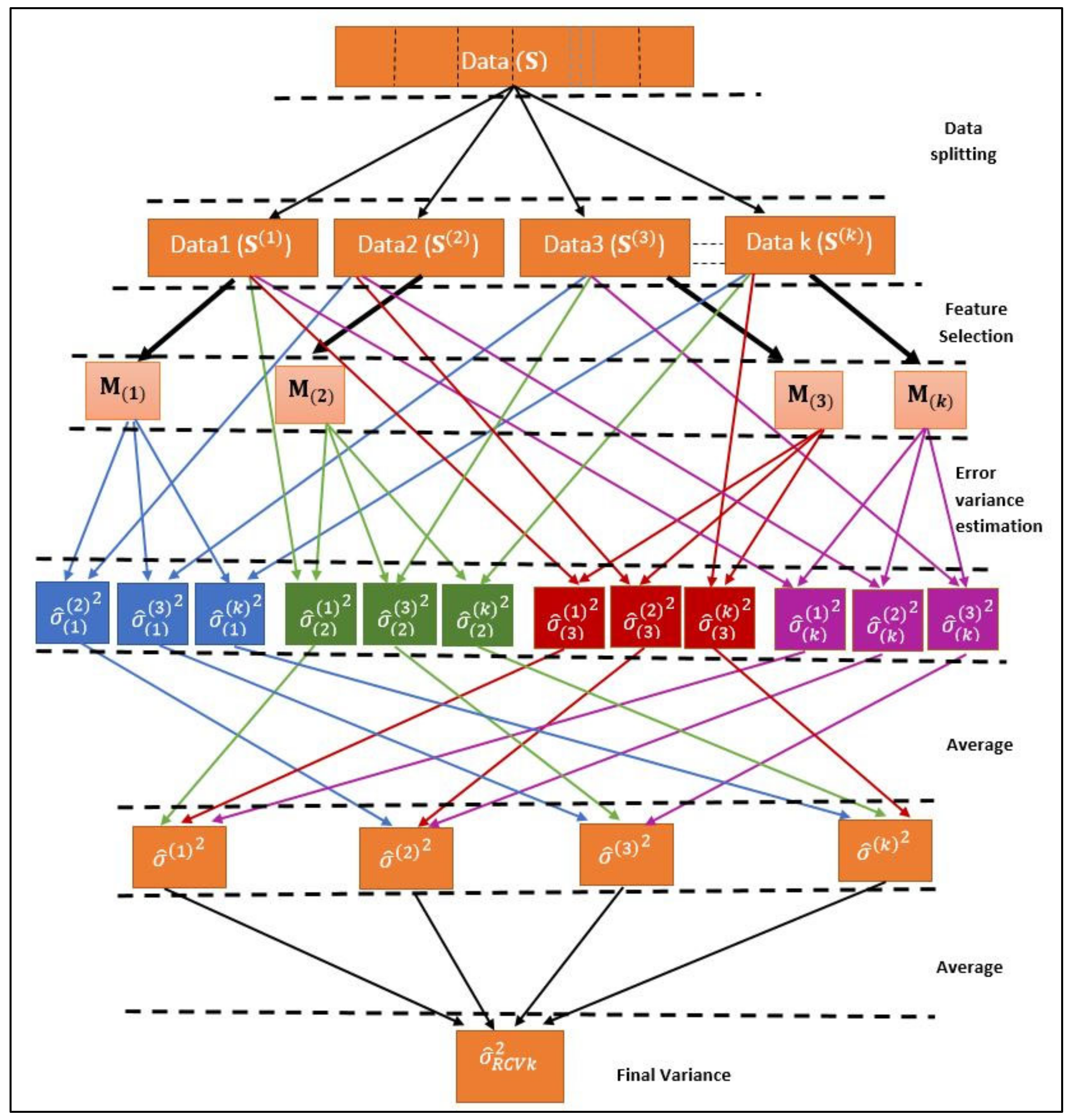
k-fold RCV is an extended version of the original RCV method [2]. In this case, the data is divided into k equal size groups instead of 2 groups. Variables are selected from one group and variance is estimated from rest of the k-1 groups. Likewise, all the groups are covered and, in the end, the average value of all the variances from each group is the final error variance (Figure 2). The algorithm is described below.

• Consider a dataset $\left(X_{n\times p},Y_{n\times 1}\right)$;
• The dataset is divided into k groups of size $m\times p$ so that $mk=n$. The new datasets are denoted as $S^{\left(i\right)}=\left(X_{m\times p}^{\left(i\right)},Y_{m\times 1}^{\left(i\right)}\right)$, $i=1,2,\dots ,k$;
• Let $S=\left\{S^{\left(i\right)}\right\}$,$i=1,2,\dots ,k$, and $S^{\left(i\right)}$ denotes the ith subsample;
• $S_{\left(i\right)}=S-S^{\left(i\right)}$, i.e., $S_{\left(i\right)}$ is a subset of $S$ excluding $i$th subsample;
• Variable selection has been done on all subsamples of set $S_{\left(i\right)}$;
• $V_{\left(i\right)}$ is a set of selected variables on subsample $S_{\left(i\right)}$, written as $V_{\left(i\right)}=\left\{M_{\left(r\right)}\right\}$, $i,r=1,2,\dots ,k$ and $r\ne i$, where $M_{\left(r\right)}$ is set of selected variables from subsamples $S^{\left(i\right)}$, ($i\ne r$);
• Now, the ordinary least squares method is used to estimate variance in $S^{\left(i\right)}$ using only the selected variables $V_{\left(i\right)}$. Thus, we get $k-1$ variances i.e., one each from $S^{\left(i\right)}$, $i=1,2,\dots ,k$−1.

  $${{\widehat{\sigma }}_{\left(r\right)}^{\left(i\right)}}^2=\frac{{Y^{\left(i\right)}}^T\left(I_{\frac{n}{k}}-P_{M_{\left(r\right)}}^{\left(i\right)}\right)Y^{\left(i\right)}}{\frac{n}{k}-\left|M_{\left(r\right)}\right|}$$

  where $P_{M_{\left(r\right)}}^{\left(i\right)}=X_{M_{\left(r\right)}}^{\left(i\right)}{\left({X_{M_{\left(r\right)}}^{\left(i\right)}}^T{X}_{M_{\left(r\right)}}^{\left(i\right)}\right)}^{-1}{X_{M_{\left(r\right)}}^{\left(i\right)}}^T$

  $${{\widehat{\sigma }}^{\left(i\right)}}^2=\frac{1}{k-1}{\displaystyle \sum }_{r=1}^{k-1}{{\widehat{\sigma }}_{\left(r\right)}^{\left(i\right)}}^2$$
• So, the final estimator of variance is

  $${\widehat{\sigma }}_{RCVk}^2=\frac{1}{k}{\displaystyle \sum }_{i=1}^k{{\widehat{\sigma }}^{\left(i\right)}}^2$$

Variables are selected in step v with the help of three feature selection methods separately using SpAM, LASSO and Least Squares Regression models. Let error variance estimator of SpAM, LASSO and Least Squares Regression is represented by ${\widehat{\sigma }}_{Sp}^2$, ${\widehat{\sigma }}_{LASSO}^2$ and ${\widehat{\sigma }}_{LSR}^2$ respectively. In the above algorithm, ${\widehat{\sigma }}_{RCVk}^2$ represents ${\sigma }_{Sp}^2$, ${\widehat{\sigma }}_{LASSO}^2$ and ${\widehat{\sigma }}_{LSR}^2$ This means all the three variances from three models (${\sigma }_{Sp}^2$, ${\widehat{\sigma }}_{LASSO}^2$ and ${\widehat{\sigma }}_{LSR}^2$) will be obtained by following above algorithm of k-RCV.

2.3.3. Proposed Algorithm for Error Variance Estimation

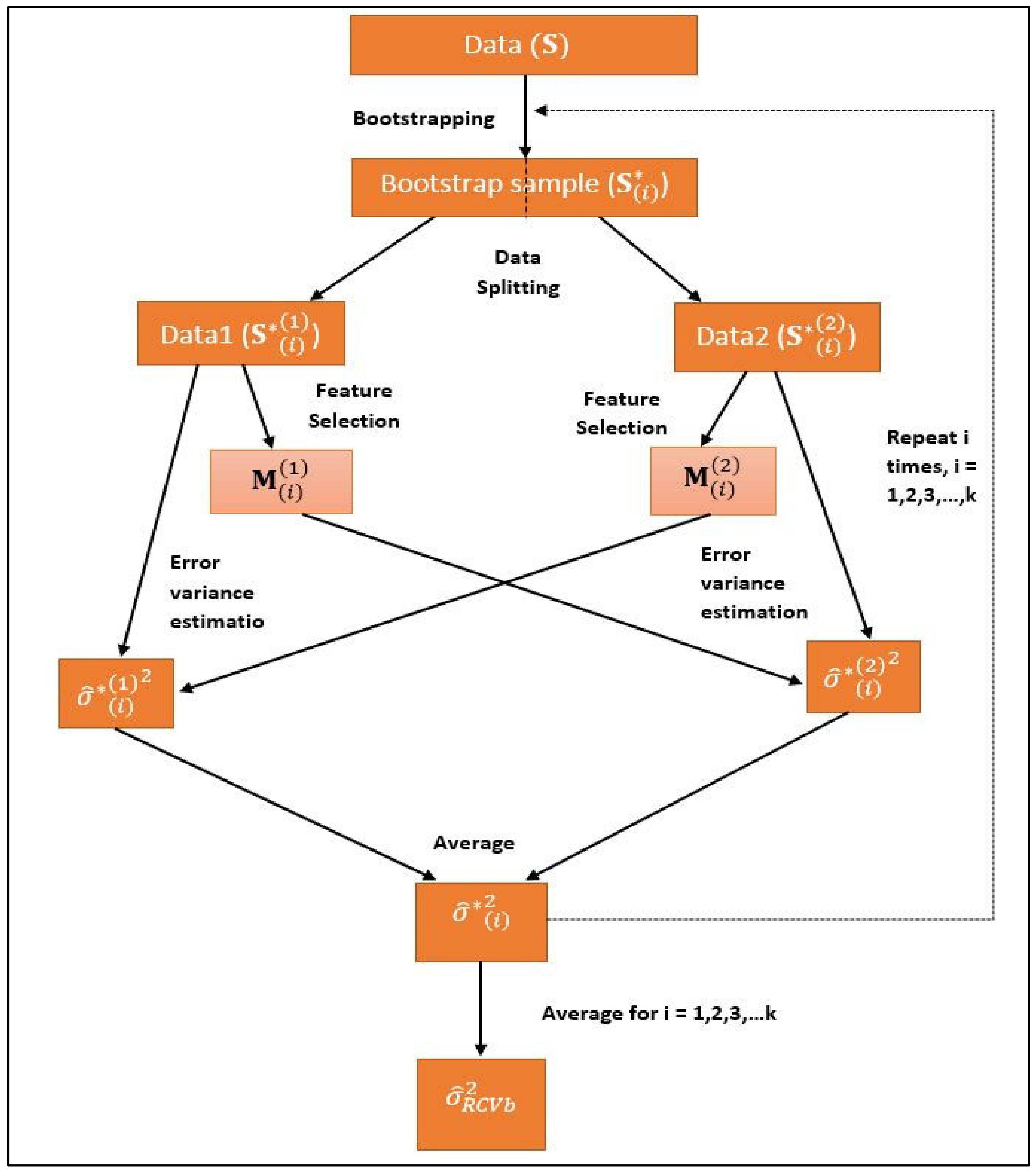
Bootstrap with RCV

In this method, bootstrap samples are taken from the original datasets and then RCV method is applied to each of these bootstrap samples (Figure 3). The algorithm for this method can be written as:

• Consider a dataset $\left(X_{n\times p},Y_{n\times 1}\right)$. We denote it as $S$;
• A bootstrap sample is selected by drawing a sample of size n by simple random sampling with replacement from the actual dataset $S$. The bootstrap sample is denoted by $S_{\left(i\right)}^{*}=\left(X^{*}{}_{n\times p}^{\left(i\right)},Y^{*}{}_{n\times 1}^{\left(i\right)}\right)$, $i=1,2,\dots ,k$. Thus, k numbers of bootstrap samples each of size n have been drawn, $S^{*}=\left\{S_{\left(i\right)}^{*}\right\}$;
• Now each $S_{\left(i\right)}^{*}$ is divided into two groups randomly, each subsample having size of n/2;

  $$S_{\left(i\right)}^{*}=\left\{S^{*}{}_{\left(i\right)}^{\left(1\right)},S^{*}{}_{\left(i\right)}^{\left(2\right)}\right\}$$

  where $S^{*}{}_{\left(i\right)}^{\left(1\right)}=\left(X^{*}{}_{\left(n/2\right)\times p}^{\left(1\right)},Y^{*}{}_{\left(n/2\right)\times 1}^{\left(1\right)}\right)$ and $S^{*}{}_{\left(i\right)}^{\left(2\right)}=\left(X^{*}{}_{\left(n/2\right)\times p}^{\left(2\right)},Y^{*}{}_{\left(n/2\right)\times 1}^{\left(2\right)}\right)$
• Variable selection has been performed on $S^{*}{}_{\left(i\right)}^{\left(1\right)}$ and $M_{\left(i\right)}^{\left(1\right)}$ is a set of selected variables from subsample $S^{*}{}_{\left(i\right)}^{\left(1\right)}$;
• Using only the selected variables variance is estimated in $S^{*}{}_{\left(i\right)}^{\left(2\right)}$ with ordinary least squares estimation;

  $${\widehat{\sigma }}^{*}{{}_{\left(i\right)}^{\left(1\right)}}^2=\frac{{Y^{*\left(2\right)}}^T\left(I_{\frac{n}{2}}-P_{M_{\left(i\right)}^{\left(1\right)}}^{\left(2\right)}\right)Y^{*\left(2\right)}}{\frac{n}{2}-\left|M_{\left(i\right)}^{\left(1\right)}\right|}$$

  where $P_{M_{\left(i\right)}^{\left(1\right)}}^{\left(2\right)}=X_{M_{\left(i\right)}^{\left(1\right)}}^{*\left(2\right)}{\left({X_{M_{\left(i\right)}^{\left(1\right)}}^{*\left(2\right)}}^T{X}_{M_{\left(i\right)}^{\left(1\right)}}^{*\left(2\right)}\right)}^{-1}{X_{M_{\left(i\right)}^{\left(1\right)}}^{*\left(2\right)}}^T$.
• In the next stage, variable selection has been performed on $S^{*}{}_{\left(i\right)}^{\left(2\right)}$ and $M_{\left(i\right)}^{\left(2\right)}$ is a set of selected variables from subsample $S^{*}{}_{\left(i\right)}^{\left(2\right)}$;
• Using only the selected variables variance is estimated in $S^{*}{}_{\left(i\right)}^{\left(1\right)}$ with ordinary least squares estimation;

  $${\widehat{\sigma }}^{*}{{}_{\left(i\right)}^{\left(2\right)}}^2=\frac{{Y^{*\left(1\right)}}^T\left(I_{\frac{n}{2}}-P_{M_{\left(i\right)}^{\left(1\right)}}^{\left(1\right)}\right)Y^{*\left(1\right)}}{\frac{n}{2}-\left|M_{\left(i\right)}^{\left(2\right)}\right|}$$

  where $P_{M_{\left(i\right)}^{\left(2\right)}}^{\left(1\right)}=X_{M_{\left(i\right)}^{\left(2\right)}}^{*\left(1\right)}{\left({X_{M_{\left(i\right)}^{\left(2\right)}}^{*\left(1\right)}}^T{X}_{M_{\left(i\right)}^{\left(2\right)}}^{*\left(1\right)}\right)}^{-1}{X_{M_{\left(i\right)}^{\left(2\right)}}^{*\left(1\right)}}^T$
• For $S_{\left(i\right)}^{*}$,we get the estimator of variance as

  $${\widehat{\sigma }}^{*}{}_{\left(i\right)}^2=\frac{{\widehat{\sigma }}^{*}{{}_{\left(i\right)}^{\left(1\right)}}^2+{\widehat{\sigma }}^{*}{{}_{\left(i\right)}^{\left(2\right)}}^2}{2}$$
• The final estimator of variance is

  $${\widehat{\sigma }}_{RCVb}^2=\frac{1}{k}{\displaystyle \sum }_{i=1}^k{\widehat{\sigma }}^{*}{}_{\left(i\right)}^2$$

Variable selection is performed with the help of three feature selection methods separately using SpAM, LASSO and Least Squares Regression models. Let error variance estimator of SpAM, LASSO and Least Squares Regression is represented by ${\widehat{\sigma }}_{Sp}^2$, ${\widehat{\sigma }}_{LASSO}^2$ and ${\widehat{\sigma }}_{LSR}^2$, respectively. In the above algorithm, ${\widehat{\sigma }}_{RCVb}^2$ represents ${\sigma }_{Sp}^2$, ${\widehat{\sigma }}_{LASSO}^2$ and ${\widehat{\sigma }}_{LSR}^2$. This means all the three variances from three models (${\sigma }_{Sp}^2$, ${\widehat{\sigma }}_{LASSO}^2$ and ${\widehat{\sigma }}_{LSR}^2$) will be obtained by following the above algorithm of bootstrap-RCV.

Ensemble Method

In this method, both bootstrapping and simple random sampling without replacement are combined to estimate error variance. Variables are selected from the original datasets, and all possible samples of a particular size are taken from the selected variables set with simple random sampling without replacement. With these samples of selected variables, error variance is estimated from bootstrap samples of the original datasets using the Least Squares Regression method. Finally, the average of all the estimated variances is considered the final estimate of the error variance (Figure 4). The algorithm is as follows:

• Consider a dataset $\left(X_{n\times p},Y_{n\times 1}\right)$. We denote it as $S$;
• A bootstrap sample is selected by drawing a sample of size n by simple random sampling with replacement from the actual dataset $S$. The bootstrap sample is denoted by $S_{\left(i\right)}^{*}=\left(X^{*}{}_{n\times p}^{\left(i\right)},Y^{*}{}_{n\times 1}^{\left(i\right)}\right)$, $i=1,2,\dots ,k$. Thus, k numbers of bootstrap samples each of size n have been drawn, $S^{*}=\left\{S_{\left(i\right)}^{*}\right\}$;
• Variable selection has been performed on $S$ and $M^{\left(1\right)}$ is a set of selected variables from $S$;
• All possible subsamples of size ($\left|M^{\left(1\right)}\right|/2)$ is drawn from $M^{\left(1\right)}$ by simple random sampling without replacement. The subsamples of these selected variables are denoted by ${M^{\left(r\right)}}^{\prime }$, $r=1,2,\dots ,L$;
• Using only the subsample of selected variables, i.e., ${M^{\left(r\right)}}^{\prime }$, variance is estimated in $S_{\left(i\right)}^{*}$ with ordinary least squares estimation;

  $${{\widehat{\sigma }}_{\left(i\right)}^{\left(r\right)}}^2=\frac{{Y^{*\left(i\right)}}^T\left(I_n-P_{{M^{\left(r\right)}}^{\prime }}^{\left(i\right)}\right)Y^{*\left(i\right)}}{n-\left|{M^{\left(r\right)}}^{\prime }\right|}$$

  where $P_{{M^{\left(r\right)}}^{\prime }}^{\left(i\right)}=X_{{M^{\left(r\right)}}^{\prime }}^{*\left(i\right)}{\left({X_{{M^{\left(r\right)}}^{\prime }}^{*\left(i\right)}}^T{X}_{{M^{\left(r\right)}}^{\prime }}^{*\left(i\right)}\right)}^{-1}{X_{{M^{\left(r\right)}}^{\prime }}^{*\left(i\right)}}^T$
• The estimated variance for all ${M^{\left(r\right)}}^{\prime }$ is

  $${{\widehat{\sigma }}_{\left(i\right)}}^2=\frac{1}{L}{\displaystyle \sum }_{r=1}^L{{\widehat{\sigma }}_{\left(i\right)}^{\left(r\right)}}^2$$
• The final estimator of variance is

  $${\widehat{\sigma }}_{ensemble}^2=\frac{1}{k}{\displaystyle \sum }_{i=1}^k{{\widehat{\sigma }}_{\left(i\right)}}^2$$

Variables are selected with the help of three feature selection methods separately using SpAM, LASSO and Least Squares Regression models. Let error variance estimator of SpAM, LASSO and Least Squares Regression is represented by ${\widehat{\sigma }}_{Sp}^2$, ${\widehat{\sigma }}_{LASSO}^2$ and ${\widehat{\sigma }}_{LSR}^2$, respectively. In the above algorithm, ${\widehat{\sigma }}_{ensemble}^2$ represents ${\sigma }_{Sp}^2$, ${\widehat{\sigma }}_{LASSO}^2$ and ${\widehat{\sigma }}_{LSR}^2$. This means all the three variances from the three models (${\sigma }_{Sp}^2$, ${\widehat{\sigma }}_{LASSO}^2$ and ${\widehat{\sigma }}_{LSR}^2$) will be obtained by following the above algorithm of the Ensemble method.

2.4. Development of R Package “varEst” for Implementation of the Proposed Algorithms

The objective of “varEst” package is to estimate the error variance of fitted genomic selection models from ultrahigh dimensional genomic datasets. “varEst” contains four different functions for variance estimation, viz. rcv, krcv, bsrcv and ensemble (

Table 1. Available functions in package “varEst”.

Function Name	Output
rcv	Error variance ( ${\widehat{\sigma }}_{RCV}^2$ )
krcv	Error variance ( ${\widehat{\sigma }}_{RCVk}^2$ )
bsrcv	Error variance ( ${\widehat{\sigma }}_{RCVb}^2$ )
ensemble	Error variance ( ${\widehat{\sigma }}_{ensemble}^2$ )

), which are based on four different algorithms, viz. Refitted Cross Validation (RCV), k-fold Refitted Cross Validation (k-RCV), Bootstrap with RCV and Ensemble method, respectively. In each function, there are options to choose the variable selection method among SpAM (“spam”), Least Squares Regression (“lsr”) and LASSO (“lasso”). The package “varEst” is available on CRAN at https://CRAN.R-project.org/package=varEst (accessed on 10 January 2022) for installation and use.

2.5. Application in Simulated and Real Dataset

From these simulated data sets, the GEBV was estimated using statistical models, viz. SpAM, LASSO and Linear Least Squares Regression using R. In the case of SpAM, the samQL function of the SAM package [17] was used to select 10 highly significant markers as we knew the number of true features (QTL) was 10 in each dataset. These significant markers were used for the prediction of the GEBV of the testing dataset with the help of the predict function using the SpAM fitted model on the training dataset. In order to implement the LASSO method, the glmnet function of the glmnet package [18] in R is used with default parameter values. Markers with non-zero coefficients are chosen as selected features, and among the non-zero coefficients, we can choose highly significant 10 markers on the basis of their coefficient value. In order to fit the Linear Least Squares Regression model, the approach of Meuwissen et al. (2001) was followed because, in datasets, we have more markers than the number of individuals. So, according to this approach, the simple linear regression model was fitted for each of the markers and QTL separately, i.e., we have fitted 1010 simple linear regression models. Then 100 of those markers and QTLs with the most significant p-values were selected. Further, a final linear regression model was fitted with these 100 markers simultaneously using the lm function in the stats package in R [19]. Then, from the final fitted model, 10 highly significant markers/QTLs are chosen as the final selected features. Finally, phenotypic values were predicted for testing the data set by using available marker data and estimated regression coefficient of marker effects.

In the next step, error variance was estimated for each model using four estimation methods, viz, RCV, k-RCV, bs-RCV and Ensemble. For that purpose, R functions have been used from the package “varEst” for all four methods. Moreover, the true value of error variance was estimated as we already know the true features from the simulated datasets. So, using only the true features (QTLs), the error variance was estimated with the ordinary least squares regression method. Then, the performances of the methods were compared among themselves to find the better method that could minimize the difference between the error variance estimated by the suggested methods and the true error variance.

Likewise, all four methods (viz. RCV, k-RCV, bootstrap RCV and Ensemble) have been applied in real datasets for estimation of error variance of estimating GEBV with SpAM, LASSO and Least Squares Regression.

3. Results and Discussion

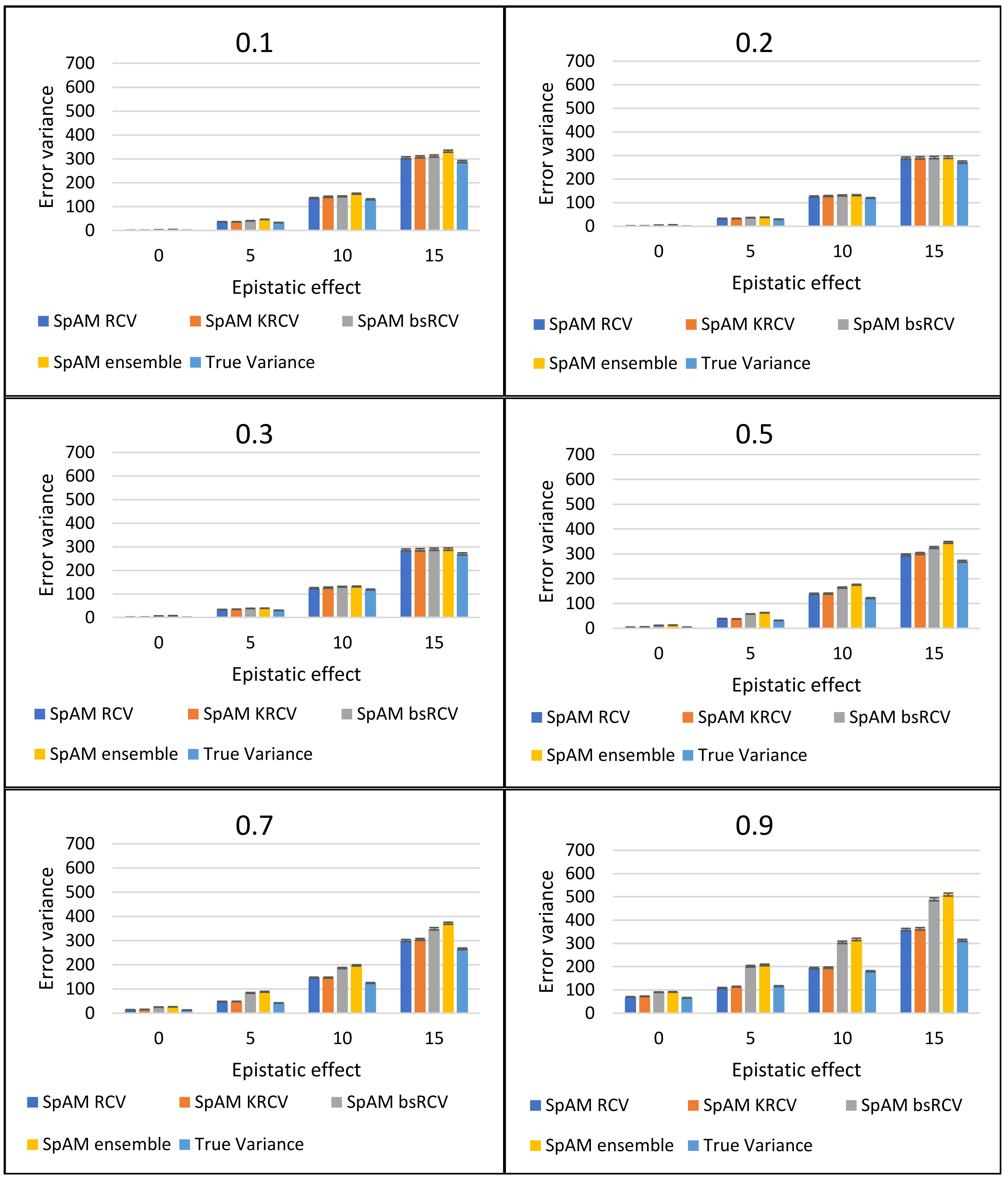
In this article, one R package called “varEst” for error variance estimation methods, viz. RCV, k-RCV, bootstrap RCV and Ensemble method has been developed. These methods have been compared on the basis of their performances in ultra-high dimensional simulated genomic datasets as well as real datasets, and the performance is evaluated for SpAM, LASSO and Least Squares Regression models. The estimated error variances from the simulated datasets are compared with the calculated true error variance of the respective datasets. The true error variance has been estimated by ordinary least squares estimate after incorporating only the true features (which is 10 QTLs in this case) into the model. The performance of SpAM is represented graphically in Figure 5. The comparison between the four error variance estimation method using SpAM as the variable (marker) selection method is shown in Figure 5. It can be observed that in a low heritability level, the Ensemble method performs better than the other three methods, whereas, in the case of higher heritability, the RCV method gives the error variance closer to the true value. It can also be observed that the error variances increase with the increase in epistatic effect in the datasets. This may be due to the fact that when the epistatic effect is present in the datasets, the additive or linear models like SpAM, LASSO, and Least Squares Regression cannot select the most relevant features (markers) from the datasets and leads to increased error variance.

In Figure 6, the performance of the four error variance estimation methods using LASSO as variable (marker) selection method are compared. It can be noticed from Figure 6 that the performances of all the error variance estimation methods have performed similar and the error variances in this case are almost same as the true error variance except in high heritability scenario (i.e., 0.7 and 0.9). Moreover, the error variances tend to increase when epistatic effect increases in the datasets.

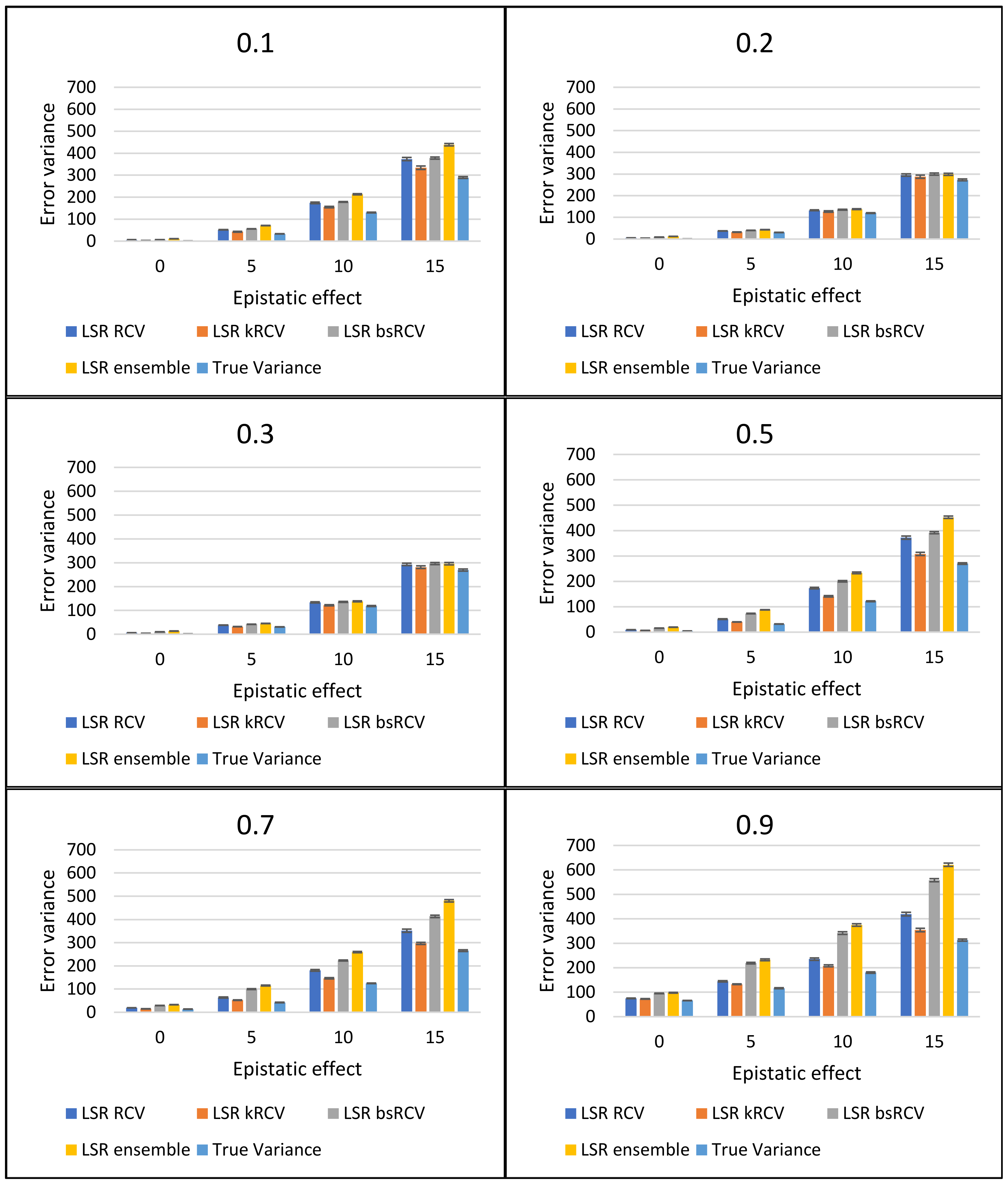
Figure 7 shows the comparative performances of RCV, k-RCV, Bootstrap RCV and Ensemble method where Least Squares Regression is used as the variable selection method in the datasets. It is observed that the k-RCV method gives the lowest value of error variance which is closer to the true variance, whereas, in case of SpAM and LASSO, the lowest value of error variance is estimated by RCV method. Like the previous cases, in this case also the error variances increase with the increase in epistatic effects in the datasets. It is also evident from the results that the error variance of LASSO is lowest among the three models, i.e., SpAM, LASSO and LSR. Though the error variance estimated by ensemble method is higher than the value of error variance estimated by RCV-based methods, the trend it follows in different genetic architectures is similar to that of RCV-based methods.

In the case of real datasets, the results are shown in

Table 2. Error variance estimation in maize dataset.

	SpAM	LASSO	LSR
RCV	-	1.4324	-
kRCV	-	1.4298	-
bsRCV	-	1.3548	-
Ensemble	1.8288	1.6590	2.5848

Note: RCV: Refitted Cross Validation, kRCV: kfold Refitted Cross Validation, bsRCV: Bootstrap RCV, LSR: Least Squares Regression, LASSO: Least Absolute Shrinkage and Selection Operator, SpAM: Sparse Additive Models.

and

Table 3. Error variance estimation in wheat dataset.

	SpAM	LASSO	LSR
RCV	0.7884	0.7965	0.7993
kRCV	-	0.7328	-
bsRCV	0.8470	0.8392	0.8319
Ensemble	1.0004	0.9993	0.9996

Note: RCV: Refitted Cross Validation, kRCV: kfold Refitted Cross Validation, bsRCV: Bootstrap RCV, LSR: Least Squares Regression, LASSO: Least Absolute Shrinkage and Selection Operator, SpAM: Sparse Additive Models.

. In real datasets, error variance could not be estimated with all the methods, such as SpAM and LSR, whereas LASSO gives results for all four methods. Basically, the problem arises in RCV and RCV-based methods due to data splitting, which is the fundamental step in the case of RCV. Here, data splitting refers to dividing the whole dataset into two or k numbers of subsets so that the sample size (i.e., n) is reduced, but the number of the predictor variable (i.e., the number of markers (p) in this case) remains same in each subset (Fan et al., 2012). In the case of genomic selection, the data we are dealing with is marker data which is categorical in nature (i.e., having values 1, 2 and 3 in our study). It has been observed that after data splitting, a singularity issue arises in matrix operations on those new subsets having a small sample size. This is because, in most cases, two or more columns become identical to each other or have the same genotype value as the number of individuals, i.e., the sample size has been reduced by data splitting. However, we can observe that the Ensemble method performs well in the case of SpAM, LASSO and also LSR in real datasets. So, we can infer that the Ensemble method can handle the shortcomings of RCV and RCV-based methods and gives an error variance estimate for all three genomic selection models. All the R scripts for data simulation and four error variance estimation methods and their results are available as Supplementary files (Script S1–S7).

Here, we have proposed four error variance estimation methods for genomic selection. There are several statistical models available for genomic selection. Some models perform well in additive genetic architecture, whereas some of them perform better in the presence of the epistatic effect. However, in the practical situation, we do not know what level of epistatic effect and additive effect is present in the data. The performances of genomic selection models are largely dependent on the genetic architecture of the data. So, it is necessary to know which statistical model to use for a particular data or particular trait. Here comes the applicability of the error variance estimation of a model. For a particular trait, we can estimate the error variance of available genomic selection models, and we can choose the model with the lowest error variance. Estimation of error variance is also helpful to know whether to use linear or non-linear genomic selection models.

4. Conclusions

In this study, four algorithms for error variance estimation in genomic selection for ultrahigh dimensional data have been suggested. These algorithms are implemented in an R package “varEst” which is made available in CRAN for free public access. The performances of the four functions available in “varEst” are evaluated based on both simulated and real datasets. From the performances of these functions, it is evident that the proposed Ensemble method can eliminate some of the shortcomings of RCV and RCV-based methods in the case of real datasets. This approach is suitable when the sample size is small. In a small sample size, using RCV and RCV-based methods are not suitable as these methods involve data splitting. The performance of the error variance estimation methods also depends on the variable selection accuracy of the genomic selection models. The models that can select more accurate variables or markers, the less is the error variance of the model. Thus, the estimation of error variance is also useful for assessing the genomic selection models.

References

- Meuwissen, T.H.E.; Hayes, B.J.; Goddard, M.E. Prediction of total genetic value using genome-wide dense marker maps. Genetics 2001, 157, 1819. [Google Scholar] [CrossRef] [PubMed]
- Fan, J.; Guo, S.; Hao, N. Variance estimation using refitted cross-validation in ultrahigh dimensional regression. J. R. Stat. Soc. Ser. B. 2012, 74, 37–65. [Google Scholar] [CrossRef] [PubMed] [Green Version]
- Fan, J.; Li, R. Variable Selection via Nonconcave Penalized Likelihood and its Oracle Properties. J. Am. Stat. Assoc. 2001, 96, 1348–1360. [Google Scholar] [CrossRef]
- Städler, N.; Bühlmann, P.; Geer, S.; Städler, N.; Bühlmann, P.; Geer, S. ℓ1-penalization for mixture regression models. TEST 2010, 19, 209–256. [Google Scholar] [CrossRef] [Green Version]
- Dicker, L.H. Variance estimation in high-dimensional linear models. Biometrika 2014, 101, 269–284. [Google Scholar] [CrossRef]
- Chen, Z.; Fan, J.; Li, R. Error Variance Estimation in Ultrahigh-Dimensional Additive Models. J. Am. Stat. Assoc. 2018, 113, 315–327. [Google Scholar] [CrossRef] [PubMed]
- Yu, G.; Bien, J. Estimating the error variance in a high-dimensional linear model. Biometrika 2019, 106, 533–546. [Google Scholar] [CrossRef]
- Liu, X.; Zheng, S.; Feng, X. Estimation of error variance via ridge regression. Biometrika 2020, 107, 481–488. [Google Scholar] [CrossRef]
- Li, Z.; Lin, W. Efficient error variance estimation in non-parametric regression. Aust. N. Z. J. Stat. 2020, 62, 467–484. [Google Scholar] [CrossRef]
- Guha Majumdar, S.; Rai, A.; Mishra, D.C. varEst: Variance Estimation, Version 0.1.0; R Package; 2019. Available online: https://CRAN.R-project.org/package=varEst (accessed on 10 January 2022).
- Yandell, B.S.; Mehta, T.; Banerjee, S.; Shriner, D.; Venkataraman, R.; Moon, J.Y.; Neely, W.W.; Wu, H.; von Smith, R.; Yi, N. R/qtlbim: QTL with Bayesian Interval Mapping in experimental crosses. Bioinformatics 2007, 23, 641–643. [Google Scholar] [CrossRef] [PubMed] [Green Version]
- Yandell, B.; Nengjun, Y.; Mehta, T.; Banerjee, S.; Shriner, D.; Venkataraman, R.; Moon, J.; Neely, W.; Wu, H.; Smith, R. qtlbim: QTL Bayesian Interval Mapping, Version 2.0.5; R Package; 2012. Available online: https://pages.stat.wisc.edu/~yandell/qtl/software/qtlbim/ (accessed on 10 January 2022).
- Kao, C.H.; Zeng, Z.B. Modeling epistasis of quantitative trait loci using Cockerham’s model. Genetics 2002, 160, 1243. [Google Scholar] [CrossRef] [PubMed]
- Crossa, J.; De Los Campos, G.; Pérez, P.; Gianola, D.; Burgueño, J.; Araus, J.L.; Makumbi, D.; Singh, R.P.; Dreisigacker, S.; Yan, J.; et al. Prediction of Genetic Values of Quantitative Traits in Plant Breeding Using Pedigree and Molecular Markers. Genetics 2010, 186, 713. [Google Scholar] [CrossRef] [PubMed] [Green Version]
- Ravikumar, P.; Lafferty, J.; Liu, H.; Wasserman, L. Sparse additive models. J. R. Stat. Soc. Ser. B 2009, 71, 1009–1030. [Google Scholar] [CrossRef]
- Tibshirani, R. Regression Shrinkage and Selection Via the Lasso. J. R. Stat. Soc. Ser. B 1996, 58, 267–288. [Google Scholar] [CrossRef]
- Zhao, T.; Li, X.; Liu, H.; Roeder, K. SAM: Sparse Additive Modelling, Version 1.0.5; R Package; 2014. Available online: https://CRAN.R-project.org/package=SAM (accessed on 10 January 2022).
- Friedman, J.; Hastie, T.; Tibshirani, R. Regularization Paths for Generalized Linear Models via Coordinate Descent. J. Stat. Softw. 2010, 33, 1–22. [Google Scholar] [CrossRef] [PubMed] [Green Version]
- R Core Team. R: A Language and Environment for Statistical Computing; R Foundation for Statistical Computing: Vienna, Austria, 2019. [Google Scholar]