Genomic Prediction of Wheat Grain Yield Using Machine Learning

Abstract

Genomic Prediction (GP) is a powerful approach for inferring complex phenotypes from genetic markers. GP is critical for improving grain yield, particularly for staple crops such as wheat and rice, which are crucial to feeding the world. While machine learning (ML) models have recently started to be applied in GP, it is often unclear what are the best algorithms and how their results are affected by the feature selection (FS) methods. Here, we compared ML and deep learning (DL) algorithms with classical Bayesian approaches, across a range of different FS methods, for their performance in predicting wheat grain yield (in three datasets). Model performance was generally more affected by the prediction algorithm than the FS method. Among all models, the best performance was obtained for tree-based ML methods (random forests and gradient boosting) and for classical Bayesian methods. However, the latter was prone to fitting problems. This issue was also observed for models developed with features selected by BayesA, the only Bayesian FS method used here. Nonetheless, the three other FS methods led to models with no fitting problem but similar performance. Thus, our results indicate that the choice of prediction algorithm is more important than the choice of FS method for developing highly predictive models. Moreover, we concluded that random forests and gradient boosting algorithms generate highly predictive and robust wheat grain yield GP models.

1. Introduction

Genomic Prediction (GP) is a methodology used to predict phenotypic values from genotypic data generated using high-throughput genotyping technologies, such as genotype-by-sequencing [1]. This observed genotype is typically recorded as single nucleotide polymorphisms (SNPs) relative to a reference genome. GP is potentially useful not only for understanding the basic genetic architecture of genomes but also for increasing the genetic performance of crops and livestock. In fact, GP is having a substantial impact on plant and animal breeding [2,3,4] because of its ability to unveil complex traits such as yield or disease/pest resistance directly from genotypes.

In GP modelling, the typical approach to choose the best method for single or multi-trait problems is to apply and compare different computational methods, namely from statistics, machine, and deep learning [5,6,7]. Bayesian and GBLUP approaches are the most commonly used methods in GP [8,9,10,11]. However, nowadays, machine and deep learning methods are being shown as a good alternative for GP in terms of accuracy, computational time, and cost. The most commonly used methods are random forests (RF) and gradient boosting (GB) for machine learning [12,13] and multilayer perceptron (mlp) and convolutional neural network for deep learning [14,15].

When developing a GP workflow, two of the most critical decisions are the choice of feature selection (FS) method and predictive model. Furthermore, a major challenge in developing a GP model is the ‘curse of dimensionality’ [16], as the number of genetic markers (p) is generally much greater than the number of genotyped/phenotyped individuals (n), i.e., $p>>n$. FS [17] and dimensionality reduction (DR) [18] approaches can be applied to overcome the marker dimensionality problem. Both approaches aim to reduce the high number of features in a dataset. FS identifies a subset of markers from the original data set without changing them, and DR transforms the original feature space into a lower dimension space, which may lead to some data loss. FS has three general approaches: filter, wrapper, and embedded, with multiple methods being available for each one. GP predictive models are based on Bayesian, machine learning (ML) or deep learning (DL) methods. Despite the importance of selecting both the FS method and the predictive model, there are limited studies. Refs. [19,20] have explored the interaction between these two steps of the GP workflow. Moreover, the performance of statistical and ML methods for GP is also highly dependent on the dataset, as shown by Refs. [21,22].

Crop yield and specifically wheat yield are important for food security. However, it faces multiple threats, including climate change, reductions in water availability, soil fertility, and land degradation. Genomics and GP are expected to be central in allowing crop yield to be maintained/increased, despite these challenges, and to respond to the 50% increase in food demand by 2050, as the global population reaches 9.7 billion [23]. Indeed, GP can help in reducing the time and cost of extensive phenotyping evaluation and in accelerating the genetic gain, during breeding programs, for key traits such as wheat yield. In order to help breeders and researchers to define their GP workflows, we evaluated the interaction between 4 FS methods and 12 predictive models, across 3 datasets in which the predicted phenotype is wheat yield. Our results revealed that the choice of prediction method is more relevant than the FS method choice. Moreover, we show that ML tree-based methods, RF, and GB are highly predictive and are the least sensitive to factors such as different FS methods, datasets, or over/under-fitting issues.

2. Materials and Methods

2.1. Dataset Description

We used a subset of the genomic and phenotypic data published by Ref. [24] to investigate the relationship between wheat genotype and the grain yield phenotype. Briefly, the datasets used in this paper consist of the following three populations: an F5 biparental population in which grain yield was measured in Pullman (WA, USA) in 2017 (501 lines; referred to as dataset1) and two double haploid biparental populations with the phenotype measured during 2018 in Pullman (759 lines; dataset2) and Lind (447 wheat lines; dataset3; WA, USA). A set of 11,089 high-quality SNPs were used for analysis. Phenotypic data is adjusted yield (measured in t/ha), calculated using an Augmented Complete Block Design from measurements obtained by harvesting whole plots.

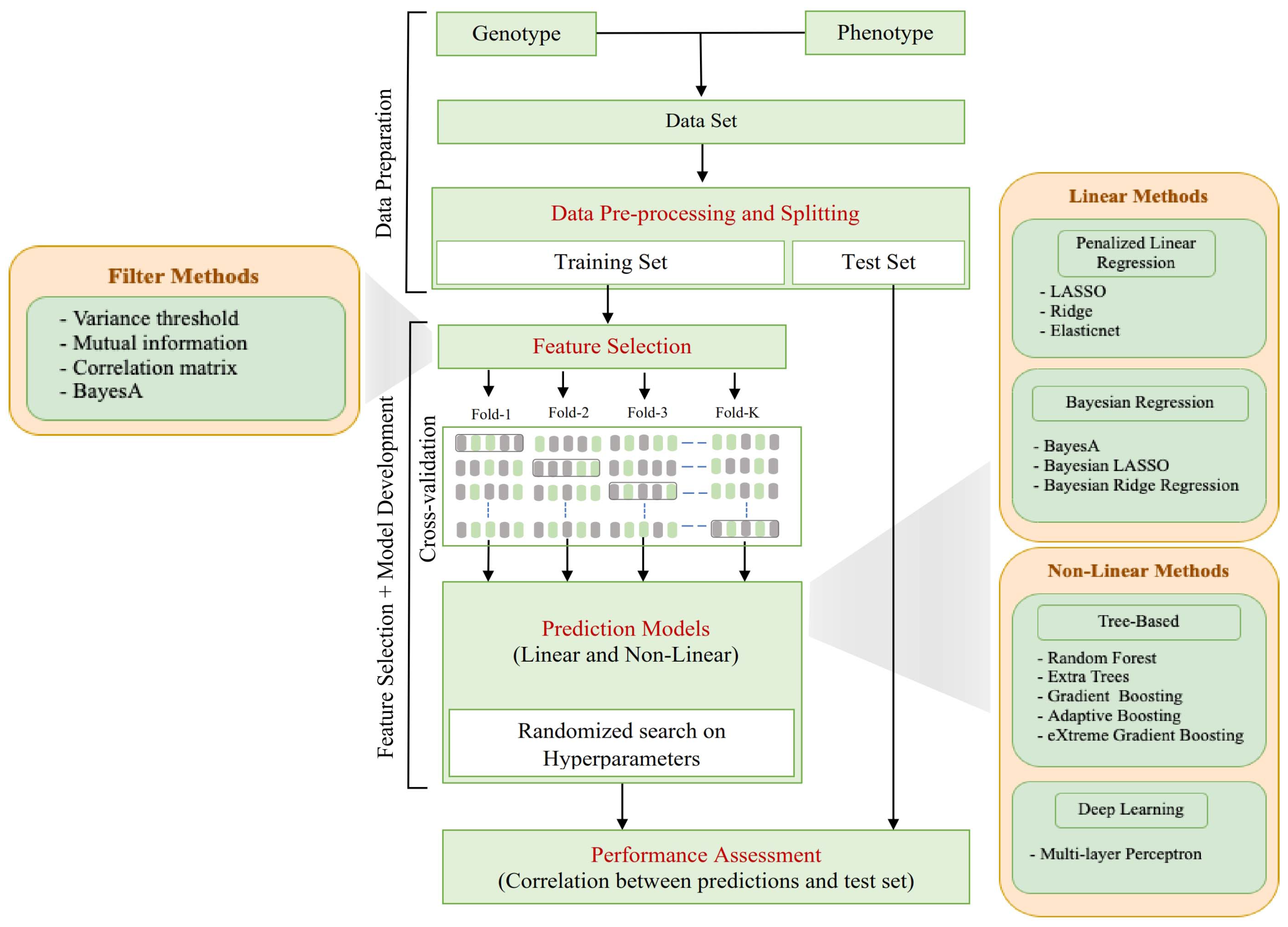
2.2. Computational Pipeline Overview

The computational pipeline can be subdivided into four main steps: (i) data pre-processing and splitting; (ii) FS; (iii) building prediction models; (iv) performance assessment, as explained in Section 2.3, Section 2.4, Section 2.5, and Section 2.6, respectively. Each of these steps were applied independently to each of the datasets described above. The framework of our study is presented in Figure 1.

2.3. Data Pre-Preprocessing and Splitting

Firstly, we accessed genotypic (input variables) and phenotypic (response variable) data using the pandas library [25], and pre-processed the data by checking for missing values using isnull function [26]. We then generated random partitions using the train_test_split helper function [27], selecting 80% of the data for training and 20% for testing for dataset1 and dataset2. For dataset3, we split into 70%/30% for training/testing. The data splitting was based on the best fitting for each dataset. After data splitting, we implemented FS approaches, as explained in Section 2.4.

2.4. Feature Selection

To investigate the best FS approach for GP of wheat grain yield, we implemented four filter methods typically used after data pre-processing: variance threshold (VT), mutual information (MI), correlation matrix (Corr_Matrix), and BayesA [28]. FS was conducted on the training data only because it increases prediction accuracy and reduces the over-fitting problem [29]. We used the sklearn FS library [30] to implement VT and MI methods. The VT algorithm only works on predictors but not response variables, filtering out all low-variance features ([31]). It drops the features whose variance does not meet the defined threshold, which was equal to 0.75 for dataset1 and dataset3 and 0.90 for dataset2. The Corr_Matrix used a Pearson’s correlation based on a heuristic function to determine significant features and was implemented using the $corr$ function of the pandas library. It generates a correlation matrix and removes the features with correlation greater than the threshold, which was set to 0.80 for the three datasets [32].

Unlike previous approaches, MI depends on non-parametric methods based on entropy assessment from k-nearest neighbors distances [33,34]. In particular, it measures how much information is communicated on average in one feature in relation to another. We selected the top 10% features for each dataset. Finally, BayesA is an approach often used for FS in GP studies [21]. It is an adaptive variable shrinkage method that uses t-scaled prior and a point mass at 0 to select informative features [35,36]. In our experiments, we draw the top 5500 features (50% of total features) in each dataset, selected by BayesA method, which was implemented using R based BGLR library [37]. In order to decide the best thresholds and top feature sets for (VT and Corr_Matrix) and BayesA, respectively, we generated feature sets on different threshold and feature set values, trained the models on those feature sets, and explored the best threshold for each dataset.

2.5. Prediction Models

We chose 12 regression methods, categorized them into linear and non-linear, and belonging to 4 computational families. In the linear category, we selected three classical benchmark approaches (i.e., Bayesian regression family), which we considered as baseline models, and three approaches from the penalized regression family. In the non-linear category, we studied five approaches from the tree-based family and one from the DL family. We trained a collection of 12 models per dataset, using the feature (SNP) sets selected by each FS method. Thus, we performed a total of 144 experiments (12 predictive methods × 4 FS methods × 3 datasets).

We used k-fold cross-validation (CV) re-sampling strategy to validate the models. Hence, the training data were randomly partitioned into k equally sized data subsets [38]. Random search is a method widely used over a set of parameters, in which each setting is sampled from a distribution over possible settings [39]. Therewith, a set of k − 1 data points are used for training and the remaining partition for validation. Afterward, we used a 4-fold randomized search CV on the k−1 training data points to select the optimized set of hyper-parameters [40]. Each model was trained using the optimized hyper-parameter set. The prediction models were implemented using Python [41] and R languages [42], so we denoted model names with ‘py’ or ‘r’. The different models were implemented with the following tools:

1.

Tree-based: Random Forests (RF_py), extraTrees_py, Gradient Boosting (GB_py) and adaboost_py with the scikit-learn ensemble library [30,43], and eXtreme gradient boosting (Xgboost_py) with XGBoost library [44];

2.

Penalized linear regression: LASSO_py, ridge_py, and elasticnet_py with the scikit-learn linear model library [30];

3.

Deep learning: Multilayer Perceptron (mlp_py) with Keras library [45];

4.

Bayesian Methods: BayesA_r, Bayesian Ridge Regression (BRR_r), and Bayesian LASSO (BL_r) were implemented with the BGLR R library [36].

Details about each prediction model and optimized hyper-parameters are described in the Supplemental Materials, Section S1.

2.6. Performance Assessment

The predictive ability of the models was compared using Pearson’s correlation coefficient (R) as a performance metric [46]. This performance metric was used for model selection on the 4-fold CV and to validate the robustness of our results by regressing the real against the predicted values on the test dataset. R is the most commonly used metric for GP problems, and it is typically defined as:

$$R=\frac{\sum (x-\overline{x})(y-\overline{y})}{\sqrt{\sum {(x-\overline{x})}^2\sum {(y-\overline{y})}^2}},$$

(1)

where x and y are the real and predicted variables, respectively. The calculation of the p-value relies on the assumption that each dataset is normally distributed. Similar to other correlation coefficients, R varies between −1 and +1, with 0 implying no correlation.

Test R values were also used as the dependent variable in linear mixed effects models, which were fitted with the nlme [47] R package, in order to assess the effect of the FS methods and the prediction models on R. In these models, each dataset was fitted as a random effect and each model was minimized following stepwise deletion of the least significant terms, with log-likelihood ratio (${\chi }^2$) tests being used to evaluate the change in model deviance, keeping only significant terms.

3. Results and Discussion

3.1. Feature Selection Methods Vary Widely in the Number and Identity of the Selected SNPs

The GP framework requires selecting the most appropriate FS method after data processing. We tested four FS methods that showed a broad variation in selected SNP numbers.

VT and Corr_Matrix methods chose a variable number of SNPs depending on the dataset. The number of SNPs selected by the VT and Corr_Matrix methods varied from 2417 (22%) to 4700 (42%) and from 3169 (29%) to 4714 (42%), respectively (

Table 1. List of selected features by each feature selection method per dataset.

Feature Selection	Dataset1	Dataset2	Dataset3
VT	3235	2417	4700
MI	1109
Corr_Matrix	4714	3835	3169
BayesA	5500

). Conversely, MI and BayesA selected SNPs were fixed at 1109 (10% of all SNPs) and 5500 (50%), respectively. Among all methods, the selected SNPs identity showed broad variation across populations, as seen in Supplemental Figures S1–S12.

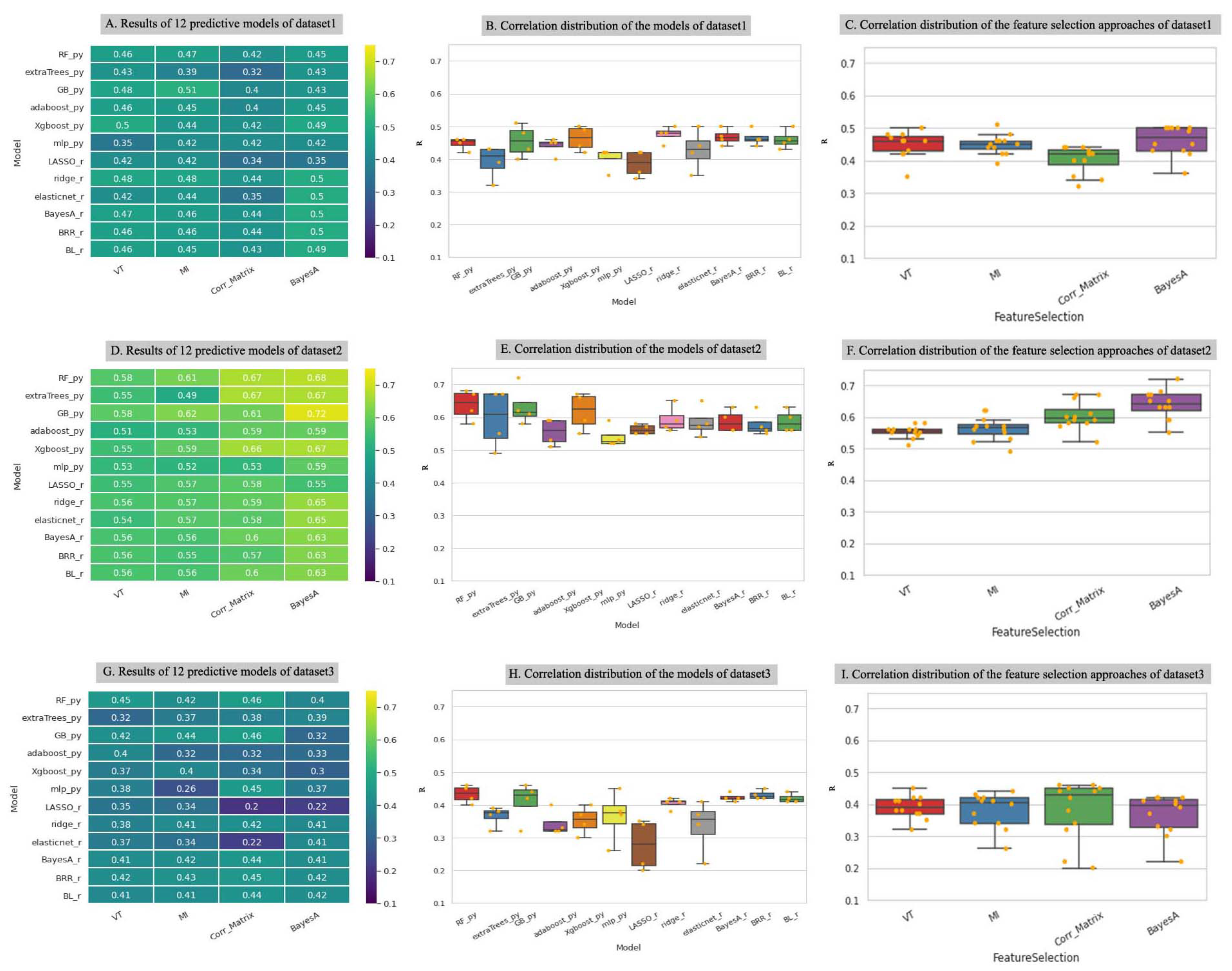
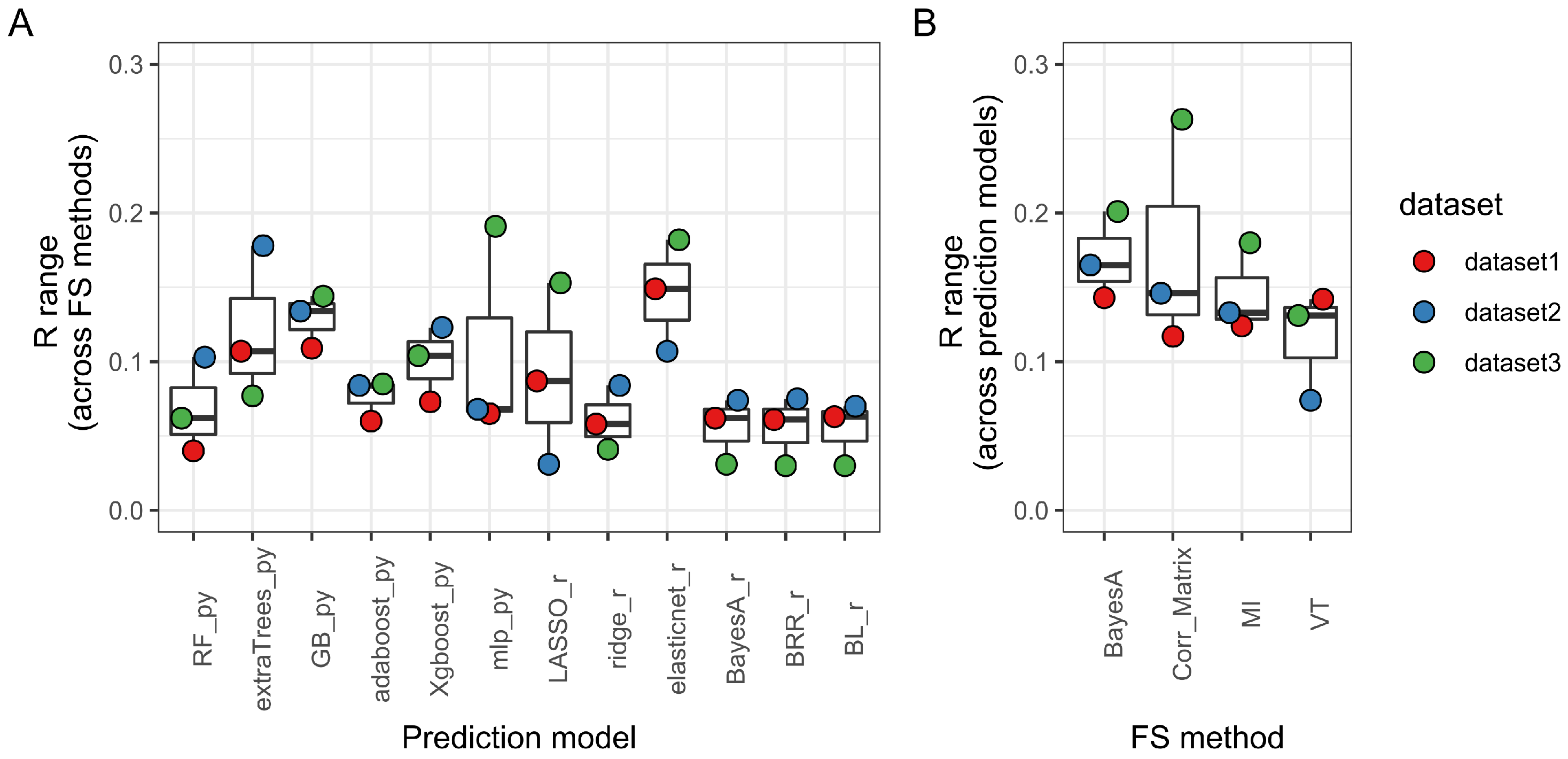
3.2. Prediction Method Is the Main Determinant of Model Performance

To assess the performance of the prediction models on the test data and its dependence on the FS method and dataset, we analyzed the statistical association between predicted and real continuous variables by accessing the performance (R) values. Across all datasets (Figure 2A,D,G), R varied between 0.20 and 0.72. The best performance was obtained for dataset2 (R between 0.49 and 0.72), which was expected as it is the largest dataset with the most wheat lines. Dataset1 analysis revealed intermediate performance (0.32 $<R<$ 0.51), and dataset3 analysis resulted in poor performance models (0.20 $<R<$0.46). Notably, dataset3 has the smallest number of wheat lines, thus highlighting the importance of sample size for prediction accuracy.

Next, we used a simple linear mixed model to better understand whether the performance (R) variation is more affected by the choice of prediction model or FS method, while controlling for the effect of the dataset size. Our results show that model performance is not significantly affected by the interaction between FS method and prediction model (${\chi }_{33}^2$ = 38.7; p = 0.23). Conversely, the choice of FS method showed only a borderline significant effect (${\chi }_3^2$ = 8.1; p = 0.04), while the prediction model choice displayed a stronger effect (${\chi }_{11}^2$ = 55.2; p< 0.0001) when analysed individually. Therewith, the prediction model affected the median R values more than the FS method (Figure 2B,C,E,F,H,I). Furthermore, R ranged dependently within each dataset on the prediction model rather than on the FS method (Figure 3). The R range across FS methods per prediction model (Figure 3A) was generally smaller than that estimated across the prediction models for a given FS method (Figure 3B). Taken together, these results suggest that both across and within the same FS approach, the prediction model choice dramatically affects the prediction accuracy.

Across all datasets, the best prediction model - FS combinations were: GB_py with MI (dataset1), GB_py with BayesA (dataset2), and GB_py or RF_py with Corr_Matrix (dataset3) (Figure 2A,D,G). This indicates that while GB_py generally led to the best prediction model, the best FS was variable, reinforcing the idea that the FS method has a minor effect on the predictability of the final model than the prediction method. Moreover, we considered optimal models those with a difference of R≤ 0.05 relative to the best model for each dataset. Within this R range, GB and RF generated at least one optimal model across all datasets. This is followed by Xgboost, ridge, elasticnet, BayesA, BRR, and BL that were in the optimal range for two datasets (dataset1 and dataset3 in all cases), and by three prediction methods that were optimal in a single dataset: adaboost (dataset1), extraTrees (dataset2), and mlp (dataset3). Interestingly, LASSO was the only method that never provided predictability within this optimal range, displaying the poorest performance for all models. This indicates that models from all four families studied here can have performances on par with the best model, but it depends on the dataset size.

Focusing on GB_py and RF_py, the results showed that the best prediction models used features selected by the same FS method, depending on the dataset (dataset1: MI; dataset2: BayesA; dataset3: Corr_Matrix). Notably, GB_py was more variable than RF_py, even though GB_py could have higher performance. The difference between the highest and lowest R values for GB_py ranged between 0.11 and 0.14 (across the three datasets), whereas this ranged between 0.05 and 0.10 for RF_py (Figure 2A,D,G). Therefore, RF_py showed to be a robust model, corroborating our previous observation that RF_py had a smaller variation among FS methods (Figure 2C,F,I). The ridge regression and three Bayesian methods had robustness similar to RF_py, with the difference between the highest and lowest R values ranging between 0.03 and 0.09. Additionally, their prediction performances placed them within the optimal model range, except for dataset2, thus suggesting a stronger dependence on the dataset than GB_py or RF_py (Figure 2A,D,G). Altogether, our results suggest that RF_py and GB_py are the most robust approaches for GP in the analyzed datasets, with the choice of FS method having limited importance.

The prediction performance superiority of RF_py and GB_py observed here is likely because these models are able to learn more complex non-linear decision boundaries in the data and handle a large number of covariates and interactions with high accuracy. This is in line with previous studies showing that RF_py and GB_py can be highly predictive, with model performance being at least on par with classical Bayesian methods [21,48]. Moreover, regarding DL methods, we found that the prediction performance of mlp_py models was generally poorer than what we observed for Bayesian prediction models (Figure 2A,D,G). A similar conclusion was made in a recent review on this topic [49]. This may be because DL-based methods require sufficiently large training data, which is not the case of the present datasets. Therefore, we concluded that RF_py and GB_py have the highest predictive abilities over other tree-based, mlp, penalized, and Bayesian methods to solve GP problems.

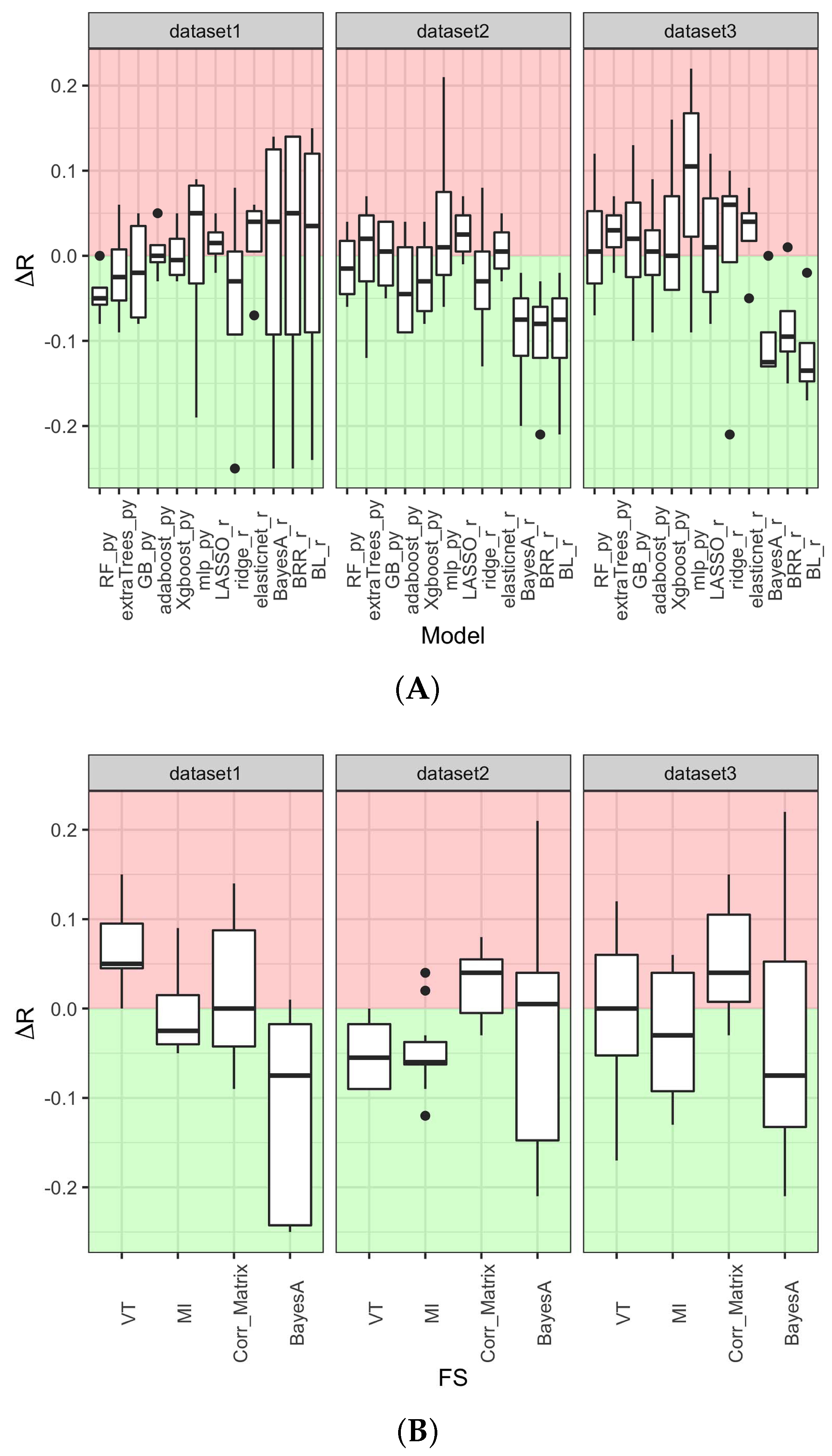
3.3. Machine Learning Tree-Based Prediction Methods Maximize Model Performance While Minimizing Over- and Under-Fitting Issues

We recorded the R-scores of the models on the training and testing datasets to understand the bias-variance trade-off [50] and see how well the models generalized to the test data. Overall, the difference in R ($\Delta R$) between test and training ranged between −0.25 and 0.22 (Figure 4). Variation in $\Delta R$ was visible both across the FS and prediction models. Regarding FS methods, models built with BayesA or MI features generally tended to under-fit, whereas the opposite occurred for Corr_Matrix. However, the range of $\Delta R$ values was substantially greater for BayesA (−0.25 to 0.22) than for Corr_Matrix (−0.09 to 0.15) or MI (−0.13 to 0.09). Conversely, the tendency for over/under-fitting for models built with VT-selected features largely depended on the dataset. Interestingly, regarding the prediction models, our results show that mlp_py ($\Delta R$: −0.19 to 0.22) and the Bayesian models ($\Delta R$: −0.25 to 0.14 for BayesA_r; −0.24 to 0.15 for BL_r; −0.25 to 0.14 for BRR_r) displayed the highest absolute and variation $\Delta R$ values, both across datasets and FS methods, regarding the prediction models.

Furthermore, the Bayesian methods tended to overfit dataset1, but underfit dataset2 and dataset3, while mlp generally showed a tendency for over-fitting, particularly on dataset3 (which is the smallest one). All tree-based methods (Xgboost_py, adaboost_py, GB_py, RF_py and extraTrees_py) and two linear methods (elasticnet_r, LASSO_r) showed a less evident tendency for over- or under-fitting (i.e., absolute $\Delta R$ ≤ 0.05). Absolute $\Delta R$ ≤ 0.05 was only observed for dataset3 for the set of models with the highest R values obtained with the test dataset, with under-fitting for RF_py and over-fitting for GB_py (Figure 2. In both cases, replacing Corr_Matrix by VT or MI would yield similarly predictive models (Figure 2G,H,I), while minimizing over- and under-fitting issues.

4. Conclusions

Machine Learning (ML) has a critical role in turning high-throughput measurements into specialized prediction models, including for the GP field [51]. We designed this study to analyse the interaction between FS and prediction methods by implementing 12 linear and non-linear methods along with 4 FS approaches. Our comparative study of the FS methods suggests that variance threshold, mutual information, and correlation matrix FS methods show more consistent results than the BayesA method. However, the choice of the prediction model has the highest impact on prediction accuracy. In this regard, our results indicate that tree-based methods achieved the highest performance (particularly GB and RF), which is also found in Ref. [48] and are the least sensitive to the choice of FS method. Moreover, among the more conventional Bayesian approaches for GP, BayesA, Bayesian ridge regression, and Bayesian LASSO had the highest performance. Nevertheless, these were not superior to the tree-based ML methods and seemed prone to over- or under-fitting issues. Thus, our results indicate that tree-based models, particularly RF and GB, are robust ML approaches for GP, across different factors (performance, robustness to FS, datasets and over- or under-fitting).

References

1. Hayes, B.; Goddard, M.; Goddard, M. Prediction of total genetic value using genome-wide dense marker maps. Genetics 2001, 157, 1819–1829. [Google Scholar] [CrossRef]
2. Bernardo, R. Molecular markers and selection for complex traits in plants: Learning from the last 20 years. Crop Sci. 2008, 48, 1649–1664. [Google Scholar] [CrossRef]
3. Scheben, A.; Yuan, Y.; Edwards, D. Advances in genomics for adapting crops to climate change. Curr. Plant Biol. 2016, 6, 2–10. [Google Scholar] [CrossRef]
4. Xu, Y.; Liu, X.; Fu, J.; Wang, H.; Wang, J.; Huang, C.; Prasanna, B.M.; Olsen, M.S.; Wang, G.; Zhang, A. Enhancing genetic gain through genomic selection: From livestock to plants. Plant Commun. 2020, 1, 100005. [Google Scholar] [CrossRef] [PubMed]
5. González-Camacho, J.M.; Ornella, L.; Pérez-Rodríguez, P.; Gianola, D.; Dreisigacker, S.; Crossa, J. Applications of machine learning methods to genomic selection in breeding wheat for rust resistance. Plant Genome 2018, 11, 170104. [Google Scholar] [CrossRef]
6. Sandhu, K.S.; Patil, S.S.; Aoun, M.; Carter, A.H. Multi-Trait Multi-Environment Genomic Prediction for End-Use Quality Traits in Winter Wheat. Front. Genet. 2022, 13, 831020. [Google Scholar] [CrossRef]
7. Farooq, M.; van Dijk, A.D.; Nijveen, H.; Mansoor, S.; de Ridder, D. Genomic prediction in plants: Opportunities for machine learning-based approaches. F1000Research 2022. [Google Scholar] [CrossRef]
8. Crossa, J.; Campos, G.D.L.; Pérez, P.; Gianola, D.; Burgueno, J.; Araus, J.L.; Makumbi, D.; Singh, R.P.; Dreisigacker, S.; Yan, J.; et al. Prediction of genetic values of quantitative traits in plant breeding using pedigree and molecular markers. Genetics 2010, 186, 713–724. [Google Scholar] [CrossRef]
9. Habier, D.; Fernando, R.L.; Kizilkaya, K.; Garrick, D.J. Extension of the bayesian alphabet for genomic selection. BMC Bioinform. 2011, 12, 186. [Google Scholar] [CrossRef]
10. Saini, D.K.; Chopra, Y.; Singh, J.; Sandhu, K.S.; Kumar, A.; Bazzer, S.; Srivastava, P. Comprehensive evaluation of mapping complex traits in wheat using genome-wide association studies. Mol. Breed. 2022, 42, 1–52. [Google Scholar] [CrossRef]
11. Meher, P.K.; Rustgi, S.; Kumar, A. Performance of Bayesian and BLUP alphabets for genomic prediction: Analysis, comparison and results. Heredity 2022, 128, 519–530. [Google Scholar] [CrossRef] [PubMed]
12. Sandhu, K.; Patil, S.S.; Pumphrey, M.; Carter, A. Multitrait machine-and deep-learning models for genomic selection using spectral information in a wheat breeding program. Plant Genome 2021, 14, e20119. [Google Scholar] [CrossRef] [PubMed]
13. Montesinos-López, O.A.; Gonzalez, H.N.; Montesinos-López, A.; Daza-Torres, M.; Lillemo, M.; Montesinos-López, J.C.; Crossa, J. Comparing gradient boosting machine and Bayesian threshold BLUP for genome-based prediction of categorical traits in wheat breeding. Plant Genome 2022, e20214. [Google Scholar] [CrossRef] [PubMed]
14. Sandhu, K.S.; Aoun, M.; Morris, C.F.; Carter, A.H. Genomic selection for end-use quality and processing traits in soft white winter wheat breeding program with machine and deep learning models. Biology 2021, 10, 689. [Google Scholar] [CrossRef] [PubMed]
15. Sandhu, K.S.; Lozada, D.N.; Zhang, Z.; Pumphrey, M.O.; Carter, A.H. Deep learning for predicting complex traits in spring wheat breeding program. Front. Plant Sci. 2021, 11, 613325. [Google Scholar] [CrossRef] [PubMed]
16. Bellman, R.E. Adaptive Control Processes: A Guided Tour; Princeton University Press: Princeton, NJ, USA, 2015; Volume 2045. [Google Scholar]
17. Chandrashekar, G.; Sahin, F. A survey on feature selection methods. Comput. Electr. Eng. 2014, 40, 16–28. [Google Scholar] [CrossRef]
18. Van Der Maaten, L.; Postma, E.; Van den Herik, J. Dimensionality reduction: A comparative. J. Mach. Learn Res. 2009, 10, 13. [Google Scholar]
19. Jain, R.; Xu, W. HDSI: High dimensional selection with interactions algorithm on feature selection and testing. PLoS ONE 2021, 16, e0246159. [Google Scholar] [CrossRef]
20. Zhou, W.; Bellis, E.S.; Stubblefield, J.; Causey, J.; Qualls, J.; Walker, K.; Huang, X. Minor QTLs mining through the combination of GWAS and machine learning feature selection. bioRxiv 2019. [Google Scholar] [CrossRef]
21. Azodi, C.B.; Bolger, E.; McCarren, A.; Roantree, M.; de Los Campos, G.; Shiu, S.H. Benchmarking parametric and machine learning models for genomic prediction of complex traits. G3 Genes Genomes Genet. 2019, 9, 3691–3702. [Google Scholar] [CrossRef]
22. Grinberg, N.F.; Orhobor, O.I.; King, R.D. An evaluation of machine-learning for predicting phenotype: Studies in yeast, rice, and wheat. Mach. Learn. 2020, 109, 251–277. [Google Scholar] [CrossRef] [PubMed] [Green Version]
23. Le Mouël, C.; Lattre-Gasquet, D.; Mora, O. Land Use and Food Security in 2050: A Narrow Road; Éditions Quae: Paris, France, 2018. [Google Scholar]
24. Lozada, D.N.; Ward, B.P.; Carter, A.H. Gains through selection for grain yield in a winter wheat breeding program. PLoS ONE 2020, 15, e0221603. [Google Scholar] [CrossRef] [PubMed]
25. Pandas—Python Data Analysis Library. Available online: https://pandas.pydata.org/ (accessed on 2 April 2021).
26. McKinney, W.; Team, P. Pandas-Powerful Python Data Analysis Toolkit. Pandas—Powerful Python Data Anal Toolkit 2015, 1625. Available online: https://pandas.pydata.org/ (accessed on 2 April 2021).
27. Géron, A. Hands-On Machine Learning with Scikit-Learn, Keras, and TensorFlow: Concepts, Tools, and Techniques to Build Intelligent Systems; O’Reilly Media: Sebastopol, CA, USA, 2019. [Google Scholar]
28. Duch, W. Filter methods. In Feature Extraction; Springer: Berlin/Heidelberg, Germany, 2006; pp. 89–117. [Google Scholar] [CrossRef]
29. Bermingham, M.L.; Pong-Wong, R.; Spiliopoulou, A.; Hayward, C.; Rudan, I.; Campbell, H.; Wright, A.F.; Wilson, J.F.; Agakov, F.; Navarro, P.; et al. Application of high-dimensional feature selection: Evaluation for genomic prediction in man. Sci. Rep. 2015, 5, 10312. [Google Scholar] [CrossRef] [PubMed]
30. Pedregosa, F.; Varoquaux, G.; Gramfort, A.; Michel, V.; Thirion, B.; Grisel, O.; Blondel, M.; Prettenhofer, P.; Weiss, R.; Dubourg, V.; et al. Scikit-learn: Machine learning in Python. J. Mach. Learn. Res. 2011, 12, 2825–2830. [Google Scholar]
31. Variance Threshold Feature Selection Using Sklearn. Available online: https://scikit-learn.org/stable/modules/generated/sklearn.feature_selection.VarianceThreshold.html (accessed on 22 June 2021).
32. Plotting a Diagonal Correlation Matrix. Available online: https://seaborn.pydata.org/examples/many_pairwise_correlations.html (accessed on 29 June 2021).
33. Kraskov, A.; Stögbauer, H.; Grassberger, P. Estimating mutual information. Phys. Rev. E 2004, 69, 066138. [Google Scholar] [CrossRef] [PubMed]
34. Vergara, J.R.; Estévez, P.A. A review of feature selection methods based on mutual information. Neural Comput. Appl. 2014, 24, 175–186. [Google Scholar] [CrossRef]
35. O’Hara, R.B.; Sillanpää, M.J. A review of Bayesian variable selection methods: What, how and which. Bayesian Anal. 2009, 4, 85–117. [Google Scholar] [CrossRef]
36. Pérez, P.; de los Campos, G. BGLR: A statistical package for whole genome regression and prediction. Genetics 2014, 198, 483–495. [Google Scholar] [CrossRef]
37. de los Campos, G.; Pataki, A.; Pérez, P. The BGLR (Bayesian Generalized Linear Regression) R-Package. 2015. Available online: http://bglr.r-forge.r-project.org/ (accessed on 8 April 2022).
38. Bengio, Y.; Grandvalet, Y. No unbiased estimator of the variance of k-fold cross-validation. J. Mach. Learn. Res. 2004, 5, 1089–1105. [Google Scholar]
39. Bergstra, J.; Bengio, Y. Random search for hyper-parameter optimization. J. Mach. Learn. Res. 2012, 13, 281–305. [Google Scholar]
40. Probst, P.; Boulesteix, A.L.; Bischl, B. Tunability: Importance of hyperparameters of machine learning algorithms. J. Mach. Learn. Res. 2019, 20, 1934–1965. [Google Scholar]
41. Sanner, M.F. Python: A programming language for software integration and development. J. Mol. Graph Model. 1999, 17, 57–61. [Google Scholar]
42. Ihaka, R.; Gentleman, R. R: A language for data analysis and graphics. J. Comput. Graph. Stat. 1996, 5, 299–314. [Google Scholar] [CrossRef]
43. Scikit-Learn Machine Learning in Python. Available online: https://scikit-learn.org/stable/ (accessed on 15 July 2020).
44. XGBoost Documentation. Available online: https://xgboost.readthedocs.io/en/latest/ (accessed on 15 July 2020).
45. Gulli, A.; Pal, S. Deep Learning with Keras; Packt Publishing Ltd.: Birmingham, UK, 2017. [Google Scholar]
46. SPSS Tutorials: Pearson Correlation. Available online: https://libguides.library.kent.edu/SPSS/PearsonCorr (accessed on 1 July 2020).
47. Pinheiro, J.; Bates, D.; DebRoy, S.; Sarkar, D.; Heisterkamp, S.; Van Willigen, B.; Maintainer, R. Package ‘nlme’. Linear Nonlinear Mixed Eff. Model. Version 2017, 3. Available online: https://CRAN.R-project.org/package=nlme (accessed on 12 June 2022).
48. González-Recio, O.; Forni, S. Genome-wide prediction of discrete traits using Bayesian regressions and machine learning. Genet. Sel. Evol. 2011, 43, 7. [Google Scholar] [CrossRef] [PubMed]
49. Montesinos-López, O.A.; Montesinos-López, A.; Pérez-Rodríguez, P.; Barrón-López, J.A.; Martini, J.W.; Fajardo-Flores, S.B.; Gaytan-Lugo, L.S.; Santana-Mancilla, P.C.; Crossa, J. A review of deep learning applications for genomic selection. BMC Genom. 2021, 22, 19. [Google Scholar] [CrossRef]
50. Belkin, M.; Hsu, D.; Ma, S.; Mandal, S. Reconciling modern machine-learning practice and the classical bias–variance trade-off. Proc. Natl. Acad. Sci. USA 2019, 116, 15849–15854. [Google Scholar] [CrossRef] [PubMed]
51. Tong, H.; Nikoloski, Z. Machine learning approaches for crop improvement: Leveraging phenotypic and genotypic big data. J. Plant Physiol. 2021, 257, 153354. [Google Scholar] [CrossRef]
52. Mendes-Moreira, J.; Soares, C.; Jorge, A.M.; Sousa; Jorge, F. Ensemble approaches for regression: A survey. ACM Comput. Surv. (CSUR) 2012, 45, 1–40. [Google Scholar] [CrossRef]
53. Breiman, L. Random Forests; Springer: Berlin/Heidelberg, Germany, 2001; Volume 45, pp. 5–32. [Google Scholar]
54. Geurts, P.; Ernst, D.; Wehenkel, L. Extremely randomized trees. Mach. Learn. 2006, 63, 3–42. [Google Scholar] [CrossRef]
55. Friedman, J.H. Greedy function approximation: A gradient boosting machine. Ann. Stat. 2001, 29, 1189–1232. [Google Scholar] [CrossRef]
56. Freund, Y.; Schapire, R.E. A decision-theoretic generalization of on-line learning and an application to boosting. J. Comput. Syst. Sci. 1997, 55, 119–139. [Google Scholar] [CrossRef]
57. Zou, H.; Hastie, T. Regularization and variable selection via the elastic net. J. R. Stat. Soc. Ser. B (Stat. Methodol.) 2005, 67, 301–320. [Google Scholar] [CrossRef]
58. Tibshirani, R. The lasso method for variable selection in the Cox model. Stat. Med. 1997, 4, 385–395. [Google Scholar] [CrossRef]
59. Park, T.; Casella, G. The bayesian lasso. J. Am. Stat. Assoc. 2008, 103, 681–686. [Google Scholar] [CrossRef]
60. de Los Campos, G.; Naya, H.; Gianola, D.; Crossa, J.; Legarra, A.; Manfredi, E.; Weigel, K.; Cotes, J.M. Predicting quantitative traits with regression models for dense molecular markers and pedigree. Genetics 2009, 182, 375–385. [Google Scholar] [CrossRef] [Green Version]
61. Yin, L.; Zhang, H.; Tang, Z.; Xu, J.; Yin, D.; Zhang, Z.; Yuan, X.; Zhu, M.; Zhao, S.; Li, X.; et al. rMVP: A memory-efficient, visualization-enhanced, and parallel-accelerated tool for genome-wide association study. Genom. Proteom. Bioinform. 2021, 19, 619–628. [Google Scholar] [CrossRef]
Figure 1. The wheat grain yield prediction scheme using SNP data and classification of the implemented methods. Four filter feature selection methods were implemented: variance threshold, correlation matrix, mutual information, and BayesA. The predictive methods are categorized into linear and non-linear and belong to four different computational families. Performance was assessed using Pearson’s correlation. The four main steps of the GP workflow are highlighted in red.
Agriculture 12 01406 g001
Figure 2. The performance of the predictive models on dataset1, dataset2, and dataset3 across the feature selection methods. (A,D,G) Heat map of obtained coefficient of determination (R) on highly predictive SNPs, selected using variance threshold (VT), correlation matrix (Corr_Matrix), mutual information (MI), and BayesA. (B,E,H) Box plot of obtained R scores, organized by prediction model. (C,F,I) Box plot of obtained R scores, organized by feature selection method.
Agriculture 12 01406 g002
Figure 3. Variation in model performance depends more on the prediction method than on the FS method. (A) Range of R values per dataset per prediction model (i.e., across FS methods). (B) Range of R values per dataset per FS method (i.e., across prediction models).
Agriculture 12 01406 g003
Figure 4. (A) Boxplot of the test and train correlation (R) score differences (i.e., Δ R on the y-axis) of the 12 prediction models of dataset1, dataset2, and dataset3. Each model name is denoted by the method name and programming platform where they are implemented. (B) Boxplot of the test and train correlation (R) score differences (i.e., Δ R on the y-axis) of the 12 prediction models of dataset1, dataset2, and dataset3 of 4 feature selection methods. VT = variance threshold, Corr_Matrix = correlation matrix, MI = mutual information.
Agriculture 12 01406 g004