
Determination of Ellipsoidal Seed–Soil Interaction Parameters for DEM Simulation


1
College of Engineering and Technology, Jilin Agricultural University, Changchun 130118, China
2
College of Biological and Agricultural Engineering, Jilin University, Changchun 130012, China
*
Author to whom correspondence should be addressed.
Agriculture 2024, 14(3), 376; https://doi.org/10.3390/agriculture14030376
Submission received: 15 January 2024
/
Revised: 16 February 2024
/
Accepted: 24 February 2024
/
Published: 27 February 2024
(This article belongs to the Special Issue Smart Mechanization and Automation in Agriculture)
Abstract
:During precision sowing, the contact process between the soil and seeds cannot be ignored. The constitutive relationship of soil is relatively complex, with characteristics such as high nonlinearity, while the contact mechanism between the soil and seeds is unclear. To better understand the contact between seeds and soil, it is necessary to establish a reasonable contact model. Ellipsoidal seeds, such as soybean, red bean, and kidney bean seeds, were adopted as research objects. In this paper, we used the discrete element method to establish an ellipsoidal seed–soil contact model. The JKR + bonding model was adopted for describing the adhesion between soil particles, and the Hertz–Mindlin new restitution (HMNS) model was used for ellipsoidal seed particles to eliminate the multiple contact point issue when modeling with the multi-sphere filling method. Moreover, both simulations and experiments were conducted to calibrate the interaction parameters between soil and seeds. The path of steepest ascent test and Box‒Behnken design (BBD) tests were also used, as well as direct shear tests. Thus, certain soil parameter values were obtained, namely the JKR surface energy was 4.436 J/m2, the normal stiffness per unit area was 2.86 × 10⁶ N/m3, the shear stiffness per unit area was 5.54 × 10⁵ N/m3, the critical normal stress was 1833 Pa, and the critical shear stress was 3332 Pa. In addition, the simulation parameters for ellipsoidal seeds were obtained from previous works. Moreover, to obtain more accurate ellipsoidal seed–soil interaction parameters, collision tests, static friction tests, and rolling friction tests were adopted. A single-factor test was used to calibrate the ellipsoidal seed–soil interaction parameters. The calibration results were as follows: the collision restitution coefficients of ellipsoidal seeds with soil were all 0.25. The static friction coefficient of soybeans with soil was 0.6, that of red beans with soil was 0.65, and that of kidney beans with soil was 0.5. The rolling friction coefficient of soybeans with soil was 0.1, that of red beans with soil was 0.14, and that of kidney beans with soil was 0.14. Finally, the rationality of parameter selection was verified through piling tests between ellipsoidal seeds and soil. The relative error of the angle of repose of soybean/soil was 2.99%, that of red bean/soil was 0.60%, and that of kidney bean/soil was 0.55%. Thus, the feasibility and rationality of the contact models between the ellipsoidal seeds and soil established in this paper, as well as the parameter selection, were verified.
1. Introduction
Precision sowing involves sowing a certain number of seeds into the soil at a certain depth according to accurate row spacing. Moreover, the seeds are covered with an appropriate amount of wet soil and moderately compressed to ensure uniform and suitable sowing. The germination environment ensures that the plants are neat, complete, and strong. In the precision sowing process, there is often contact between the soil and the working apparatus, between the seeds and the working apparatus, and between the seeds and the soil. Whether seeds can achieve desirable precision sowing also depends on the abovementioned contact effect. To analyze these contacts, building a precise contact model of seed–soil using the discrete element method is essential.
At present, the discrete element method (DEM) is often used to study the contact among particle assemblies and the contact between particle assemblies and machines. However, existing research has revealed that DEM is mostly used to study the contact between the soil and the working apparatus (subsoiling, soil covering, pressure machinery, etc.) and the contact between the seeds and the working apparatus (seed metering devices). Zhang et al. used the Hertz–Mindlin + JKR model to predict the disturbance area and traction force of tillage tools on soil. Cone penetration and uniaxial unconfined compression tests were employed to determine DEM parameters [1]. Wang et al. established a discrete element model of subsoiling and analyzed the contact effect between vibrating subsoiling machines and soil by simulating the farming process [2]. Shmulevich et al. used DEM to simulate the interaction between the soil and wide blades, and a corresponding discrete element model of the contact between the soil and blades was established [3]. Gao et al. used DEM to study the filling and separation of seed particles in a seed metering device under different conditions and analyzed the influence of various parameters [4]. Chen et al. used the discrete element simulation method to calibrate the seeding parameters for Cyperus esculentus to provide a reference for subsequent discrete element simulation of a seed metering device [5]. DEM can deal with more than one type of particle (soil particles and seeds) in an assembly. Particles displace independently of one another and interact at contacts between particles. DEM also allows particle sizes and shapes to be varied and the contact regime of a particle with surrounding particles to be monitored. However, studies on seed–soil contact have been rare. In 2014, Zhou et al. established a seed–soil contact model by using DEM [6]. They used the stiffness model to describe the contact of seed–soil, and the overlap of seed and soil particles was affected by the contact stiffness and contact force of the two contacting particles. Contact forces were determined by Newton’s force–displacement law. They only examined the contact characteristics between a single spherical particle seed and surrounding soil particles under the action of a press wheel, while the number of contact points and contact area were considered. They did not mention parameter selection for the seed–soil contact model, and the seed was simplified as a sphere without considering the contact between the seed particle assembly and soil. In 2020, Zeng and Zhou used DEM to establish a soybean cotyledon–soil contact model to simulate the germination process of a single seed [7]. The soybean cotyledon–soil dynamics were evaluated by the resistance force and system kinetic energy. However, there was no additional detailed description of the selection of soybean cotyledon–soil contact model parameters, and the research object was still a single soybean cotyledon particle. Therefore, in-depth research on soil–seed contact is urgently needed.
In addition, when using DEM to establish a contact model between ellipsoidal seeds and soil, first, it is essential to establish a contact model between ellipsoidal seeds and soil, including a geometric and mechanical model of the particles. The key to obtaining a geometric model is how to accurately express the geometric model of the particles. Generally, legume seeds are defined as spheres or ellipsoids (Boac et al., 2010) [8], and the multi-sphere filling method has been adopted for modeling. Both LoCurto et al. (1999) and Vu-Quoc et al. (2000) used the multi-sphere filling method to model individual soybean particles [9,10]. Xu (2018) [11] compared the actual shape of soybean seeds with that of standard ellipsoids, and the approximation degree between soybean seeds and standard ellipsoids was quantified based on the multi-sphere filling scheme in ellipsoidal seed partitioning modeling. In most cases, the DEM particles of soils have been modeled as spheres. Soil particles do not interlock and can rotate without dilating. Moreover, the contact calculation between spheres is simple (Dexter and Hewitt, 2006), which reduces the CPU calculation time and greatly improves the simulation efficiency [12]. Hence, for modeling dilative soils, more complex shapes, such as ellipsoids and poly-ellipsoids, are recommended because of the larger amount of time consumed due to the complex interactions during contact [13]. However, for sandy loam soil particles, there has been no unified conclusion on how to establish a geometric model.
Moreover, seeds are usually considered dry particles, and the Hertz–Mindlin (no-slip) model has been applied. However, previous research has indicated that when the multi-sphere filing method is used to establish a particle model, multiple contact points are affected [14,15,16]. The issue of multiple contact points leads to over-elasticity and over-damping of the entire system, affects particle assembly movement, and thus impacts the simulation accuracy. Zhou et al. (2020) performed simulations to propose that multiple contact points exert a significant impact on the movement of individual particles through self-flow screening and piling tests [17]. Yan et al. (2021) proposed that the impact of multiple contact points on the movement of individual particles does not affect the group behavior of the particle assembly [18]. Therefore, simply choosing the Hertz–Mindlin no-slip contact force model cannot accurately describe the movement of the ellipsoidal seed assembly or individual particles. Soils are highly nonhomogeneous and nonlinear, with complex constitutive relationships, such as moisture content, organic matter content, porosity, and texture, which greatly impact their properties. Although a large number of studies have described soil mechanics models (Mudarisov et al., 2022; Yang et al., 2024; Zhang et al., 2023 [1,19,20]), the relationships between the macroscopic and microscopic properties of soil particle assemblies are not fully understood (Jaradat and Abdelaziz, 2023; Wang et al., 2022) [21,22]. Therefore, selecting a suitable seed particle mechanics model and soil particle mechanics model requires in-depth analysis.
Meanwhile, when building a particle model, several physical and contact parameters must be obtained. Several physical and contact parameters of seeds and soil can be experimentally obtained, but some contact parameters are difficult to measure directly. Therefore, calibration tests are needed. Commonly used calibration methods include the piling test, bulk density test, direct shear test, rotating drum test, and self-flow screening test. Through comparisons between simulations and experiments, parameters can be obtained via trial and error. Hence, determining the contact parameters of the seed–soil model requires in-depth analysis.
Therefore, in this paper, DEM was used to analyze the ellipsoidal seeds–soil contact properties.
- The multi-sphere filling method was adopted to establish geometric models of ellipsoidal seeds and soil particles;
- The Hertz–Mindlin no-slip (HMNS) model was used to establish a model of ellipsoidal seed particles by considering the issue of multiple contact points. Due to the adhesion characteristics of sandy loam soil, the bonding key was added to the JKR model to simulate the contact properties of the soil;
- Through the combination of simulations and tests, the contact parameters between seeds and soil were calibrated. Both the path of steepest ascent test and Box–Behnken design (BBD) were considered, involving direct shear tests. Then, the restitution coefficient, static friction coefficient, and rolling friction coefficient between the ellipsoidal seeds and soil assembly were calibrated by a single-factor test;
- The parameter selection and established models were verified through the piling test between ellipsoidal seeds and soil.
2. Materials and Methods
2.1. Physical and Mechanical Test Analysis of Seeds
In this paper, soybean, red bean, and kidney bean seeds were adopted as the research objects, as shown in Figure 1. These three types of seeds were chosen because their shapes are similar to those of standard ellipsoids, with different aspect ratios (S = L/W).
One hundred seeds of each variety were randomly selected for three-axis dimension measurement (length L, width W, and thickness T). The measurement results are provided in Table 1.
The mechanical properties of the seeds were measured and analyzed. A universal testing machine was used for compression tests to measure the elastic modulus of the seeds, as shown in Figure 2a. The static friction coefficient of seed–seed pairs was measured using the slope method [23], as shown in Figure 2b. The simple pendulum test was employed to determine the seed–seed and seed–wall restitution coefficients [24], as shown in Figure 2c,d. Poisson’s ratio of the seeds was calculated according to the American Agricultural Association standard (a value of 0.4 is suitable for general beans) [25]. The rolling friction coefficient between the seeds and contact materials was obtained via calibration. The final parameters were selected through the Plackett–Burman test and the path of steepest ascent test combined with the piling test and rotating hub test. The results were all acquired from previous works [26].
2.2. Physical and Mechanical Test Analysis of Soil
The soil selected in this paper was sandy loam (with 21.04% gravel, 68.43% sand, and 10.46% silt). The natural density of the soil sample was measured using the ring knife method, and the density was 1950 g/cm3. Other parameters, such as the elastic modulus, Poisson’s ratio, restitution coefficient, static friction coefficient, and rolling friction coefficient, were obtained from previous works [27]. However, surface energy γ, normal contact stiffness, shear contact stiffness, critical normal stress, and critical shear stress are difficult to measure, so they were obtained through calibration, as described in Section 4.1.
3. Seed and Soil Modeling
3.1. Discrete Element Model of Seeds
Through previous work, models of ellipsoidal seeds were established based on the multi-sphere filling method, and the model accuracy was verified [26]. The specific filling models and the actual ones are shown in Figure 3.
The multiple contact point issue was considered, and the HMNS model was used to establish a contact model of ellipsoidal seeds.
3.2. Discrete Element Model of Soil
The irregular particle models in EDEM software (version 2018) were adopted to establish soil models. For example, spheres, cylinders, triangles, pie-shaped, and quadrangular pyramid soil particles were adopted. The dimensions of the soil particles ranged from 2.4 to 3.0 mm, as shown in Figure 4.
4. Determination of Contact Parameters
4.1. Calibration of Contact Parameters of Soil Models
In this section, direct shear tests were used to calibrate some of the contact parameters between the seeds and soil particles. For example, the surface energy γ of soil was included in the JKR model. Normal contact stiffness, shear contact stiffness, critical normal stress, and critical shear stress were considered in the bonding model.
4.1.1. Direct Shear Test
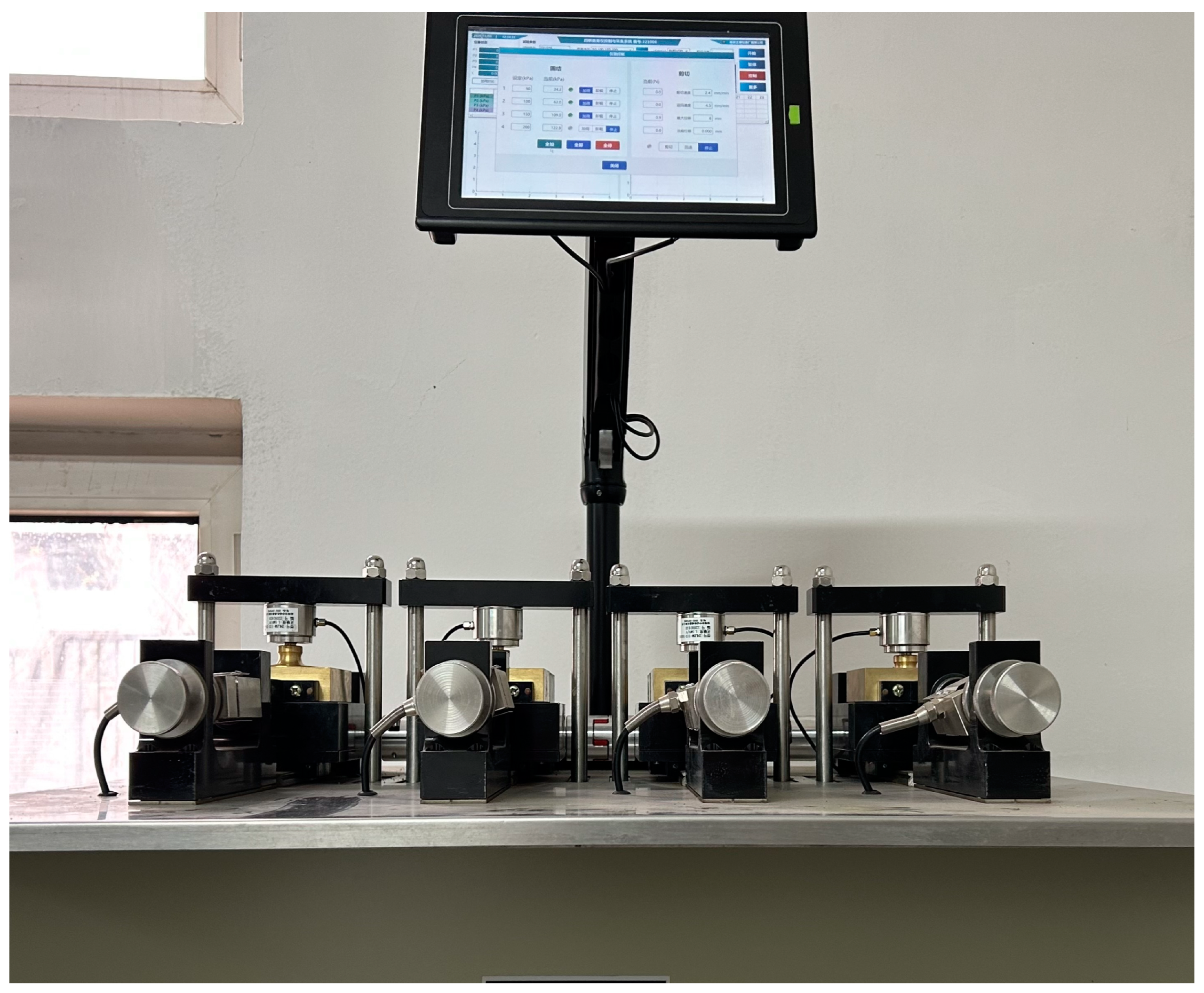
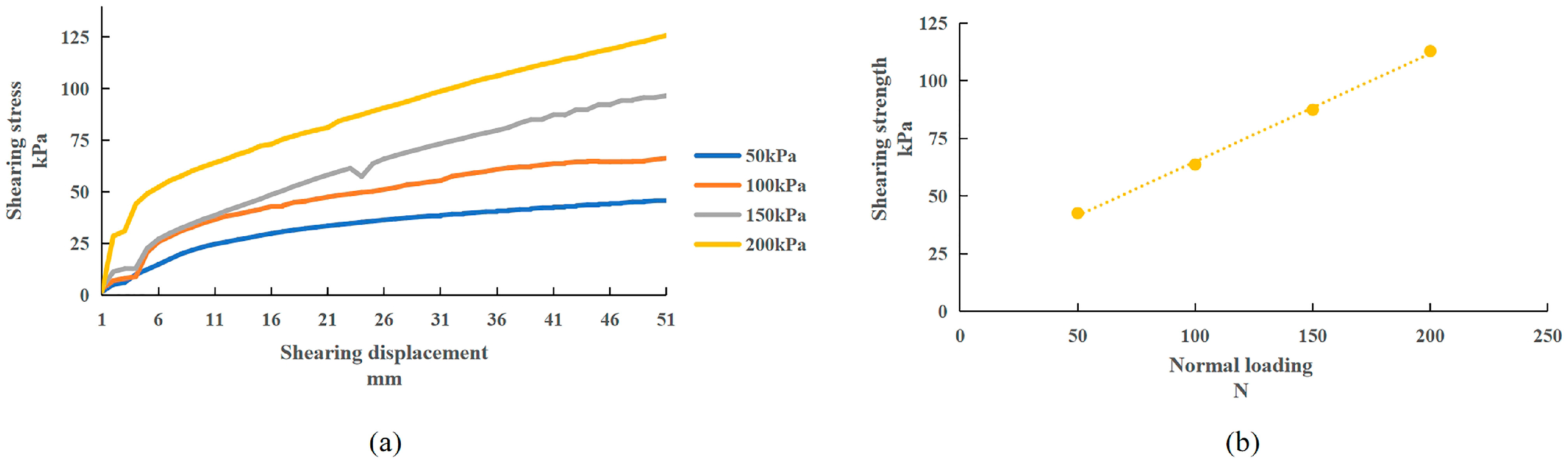
A ZJ-type fully automatic four-joint direct shear instrument was used in the direct shear test to load each sample with different normal loadings (50, 100, 150, and 200 kPa), as shown in Figure 5. In each trial, which was repeated three times, the relationship between the soil shear strength and pressure with different normal loadings could be obtained. The results are shown in Figure 6.
4.1.2. Path of Steepest Ascent Method
The value range of the path of the steepest ascent method was obtained from the literature and the test results [30,31]. In the simulation, the JKR model with a bonding key was used, and EDEM 2018 was adopted (DEM Solutions, Edinburgh, UK, 2002). The simulation time step was 5 × 10⁻⁷ s. The simulation time was 9.5 s. Soil particles were randomly generated according to the normal distribution of the volume, and the sample mass generated in the simulation matched that in the test. A simulation screenshot is shown in Figure 7.
The specific simulation arrangements and results are provided in Table 2. According to the results, given a surface energy γ of 4.5 J/m2, the normal contact stiffness was 2 × 10⁶ N/m3, the tangential contact stiffness was 6 × 10⁵ N/m3, the critical normal stress was 1800 Pa, the critical tangential stress was 3400 Pa, and the maximum shear strength was 41.1 kPa. Compared with the maximum shear strength in the physical test (42.6 kPa), the relative error was only 3.5%.
In the subsequent tests, the value of No. 2 was defined as the center point, and the values of No. 1 and No. 3 were defined as low and high points, respectively. The Box‒Behnken test was subsequently performed. The parameter levels of the Box‒Behnken test are listed in Table 3, and the test design and results are provided in Table 4. The values of the nonsignificant parameters are the same as those of the path of the steepest ascent test.
The ANOVA results for the BBD test are listed in Table 5. According to the results, for p < 0.0001, the coefficient of determination R2 = 0.9465, the adjusted coefficient of determination adjusted R2 = 0.9037 (both close to 1), and the coefficient of variation CV = 1.04%, indicating that there was a significant relationship between the response value and the parameters (p < 0.0001). Therefore, the JKR surface energy, normal stiffness per unit area, and critical normal stress significantly influenced the maximum shear strength.
Moreover, according to the relationship curve between the experimental values and the predicted values of the fitting model (in Figure 8), the data points were distributed around the fitting line, and the error was small, indicating that the model fitted well and could predict the maximum shear strength. The final values of each parameter could be obtained through BBD test analysis, namely the JKR surface energy was 4.436 J/m2, the normal stiffness per unit area was 2.86 × 10⁶ N/m3, the shear stiffness per unit area was 5.54 × 10⁵ N/m3, the critical normal stress was 1833 Pa, and the critical shear stress was 3332 Pa.
4.2. Calibration of the Contact Parameters of the Seed–Soil Model
4.2.1. Calibration of the Seed–Soil Collision Restitution Coefficient Simulation Parameter
A drop test was used to calibrate the collision restitution coefficient between the ellipsoidal seeds and soil, as shown in Figure 9. Seeds were dropped from a height of H1 = 200 mm, collision occurred between the seeds and the soil box, and the height at which the seeds bounced the most (H2) was recorded by a high-speed camera. The coefficient of restitution was calculated by . Each trial was repeated 5 times, and the mean value was obtained as the final value. The soybean/soil restitution coefficient was 0.193, the red bean/soil restitution coefficient was 0.139, and the kidney bean/soil restitution coefficient was 0.259.
Because the seed–soil and seed–seed static friction coefficients and rolling friction coefficients did not affect the bounce height, these values were set to 0 in the simulation. After the presimulation tests, the values of the seed–soil restitution coefficient were set to 0. 10, 0.15, 0.2, 0.25, 0.3, and 0.35. Six simulations were conducted. The simulation results are shown in Figure 10. The simulation results showed that with increasing restitution coefficient, the simulation results gradually fluctuated, and when the soybean–soil, red bean–soil, and kidney bean–soil restitution coefficients were all 0.25, the simulation results were closest to the experimental values. Thus, the restitution coefficient between ellipsoidal seeds and soil was 0.25.
4.2.2. Calibration of the Seed–Soil Static Friction Coefficient Simulation Parameters
The static friction coefficient was obtained by using the slope method, as shown in Figure 11. First, the soil box was placed horizontally, the seeds were placed on the soil, and the soil box was then rotated slowly and uniformly around one axis. The rotation was stopped when the upper seeds began to slip. The inclination angle θ was recorded, and the seed–soil static friction coefficient, μs, was calculated (μs = tanθ). Each trial was repeated 5 times. The mean value was adopted as the final value. Thus, the soybean/soil static friction coefficient was 0.416, the red bean/soil static friction coefficient was 0.518, and the kidney bean/soil static friction coefficient was 0.482.
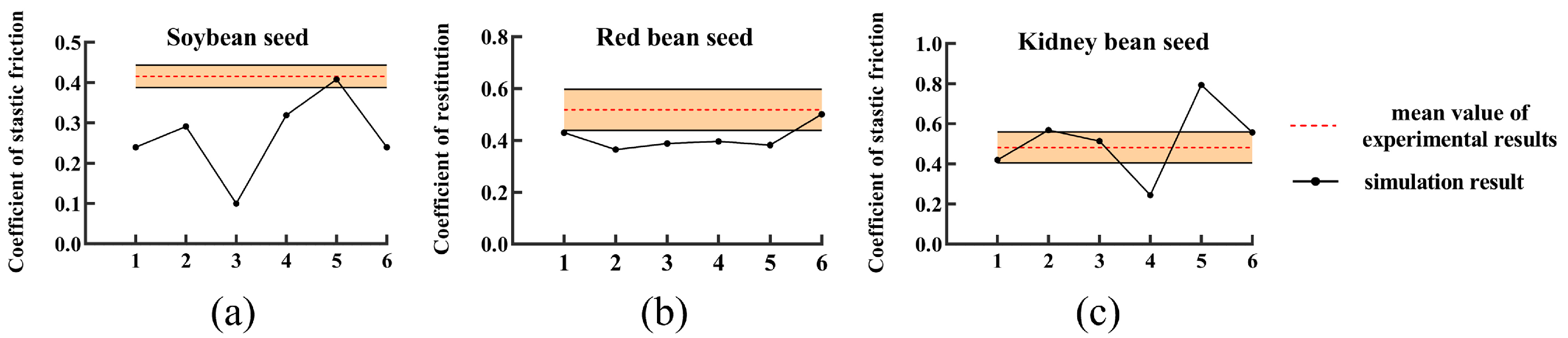
The rolling friction coefficient, the collision restitution coefficient of the seed–soil mixture, the static friction coefficient, and the rolling friction coefficient of the seed–seed mixture imposed no effect on the inclination angle. The values were all fixed at 0. The seed–soil restitution coefficient was 0.25. After the presimulation tests, the seed–soil static friction coefficients were set to 0.4, 0.45, 0.5, 0.55, 0.6, and 0.65, and six simulation tests were conducted. The simulation results are shown in Figure 12. According to the simulation results (soybean/soil, red bean/soil, and kidney bean/soil static friction coefficients of 0.6, 0.65, and 0.5, respectively), the simulation results all remained within the error band of the experimental results. Finally, the soybean/soil static friction coefficient was 0.6, the red bean/soil static friction coefficient was 0.65, and the kidney bean/soil static friction coefficient was 0.5.
4.2.3. Calibration of the Seed–Soil Rolling Friction Coefficient Simulation Parameters
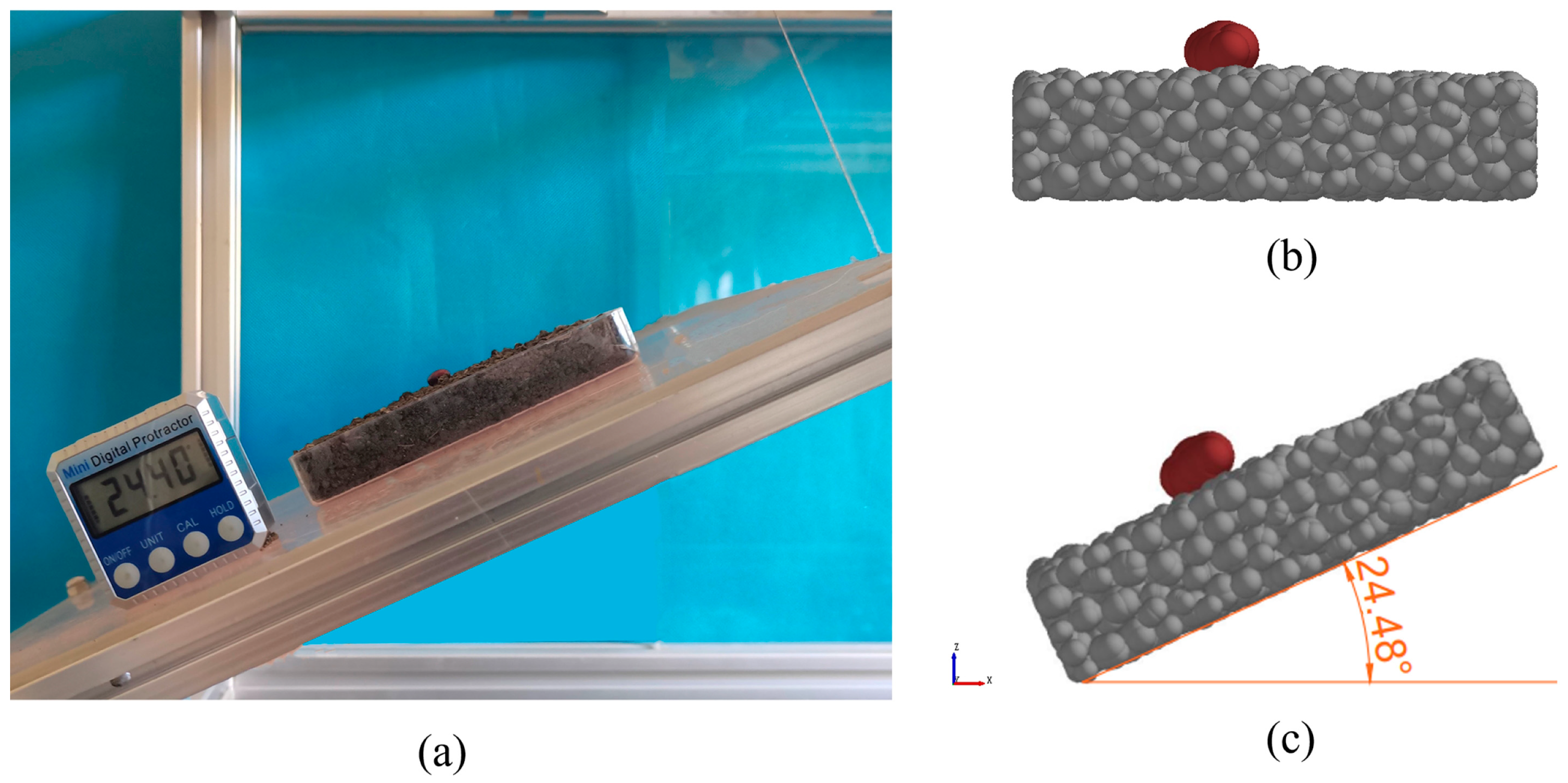
The seed–soil rolling friction coefficient was calibrated by using a slope rolling test. The test configuration is shown in Figure 13. The seeds were placed on an inclined surface with an inclination angle of 45°. The length of the inclined surface was 100 mm. The seeds rolled down the inclined surface at an initial speed of 0 from the top. The seeds eventually reached the horizontal surface, remaining completely stationary in the end, after which the horizontal rolling distance S was recorded. Each trial was repeated 7 times, and the mean value was adopted as the final value. The actual horizontal rolling distance was 29 mm for soybean seeds, 27.3 mm for red bean seeds, and 13.1 mm for kidney bean seeds.
Because the restitution coefficient, static friction coefficient, and rolling friction coefficient of the seed–seed pairs did not affect the horizontal rolling distance, the values were all set to 0. The following calibrated parameters were used: the seed–soil restitution coefficient was 0.25, the soybean/soil static friction coefficient was 0.6, that between red beans and soil was 0.65, and that between kidney beans and soil was 0.5. After the presimulation tests, the range of the seed–soil rolling friction coefficient was defined as 0.06, 0.08, 0.1, 0.12, 0.14, 0.16, 0.18, and 0.2. Eight simulation tests were also conducted. The test results are shown in Figure 14. The simulation results showed that with increasing rolling friction coefficient, the simulation results fluctuated, and for soybean–soil, red bean–soil, and kidney bean–soil rolling friction coefficients of 0.1, 0.14, and 0.14, respectively, the simulation results were all within the error band of the experimental results. Therefore, the soybean–soil rolling friction coefficient was 0.1, that between red beans and soil was 0.14, and that between kidney beans and soil was 0.14.
In summary, the values of the specific parameters in the simulation are shown in Table 6.
5. Model Accuracy Verification
5.1. Seed-Soil Piling Test
The test procedure was as follows. Prepared soil with a moisture content of 20 ± 2% was placed in a soil box with dimensions of 300 mm × 200 mm × 60 mm. Next, the seeds were loaded into the charging box. After the seed particles had stabilized, the insert plate was removed, and the seed assembly subsequently flowed out of the charging box, forming a static angle. The static repose angle was used as an indicator of the contact between the seeds and soil. Pictures of the repose angle between the seeds and soil are shown in Figure 15. The seed–soil piling test results are listed in Table 7.
5.2. Seed–Soil Piling Test Simulation
In this section, the piling tests of the three types of seeds with soil were simulated. The HMNS model was adopted for the ellipsoidal seeds. The JKR model + bonding key was used for the soil particles. The simulation time step was 5 × 10⁻⁷ s. In the piling test, the simulation time was 5 s. The simulation was conducted in three stages. In the first stage, a soil assembly was randomly generated in the soil box. In the second stage, after the soil assembly had stabilized, a seed assembly was generated with a normal distribution of the volume. The third simulation stage started when the particle assembly had stabilized for 0.5 s, the left seed plate was removed upward at a speed of 0.5 m/s, and the seed assembly subsequently formed a repose angle with the soil. The seed–soil piling test simulation process is shown in Figure 16.
A comparison between the test and simulation results is shown in Figure 17. The results showed that the simulation results were close to the experimental results. The relative error of the angle of repose of soybean/soil was 2.99%, that of red bean/soil was 0.60%, and that of kidney bean/soil was 0.55%. Therefore, the feasibility and rationality of the contact models between the ellipsoidal seeds and soil established in this paper, as well as the parameter selection, were verified.
6. Discussion
In this paper, the contact properties between ellipsoidal seeds and soil were analyzed by using DEM. Seed modeling, contact model selection, and parameters calibration were included.
6.1. Seed Modeling
Accurately representing the shape is the key to DEM analysis. More diverse geometrical particle models are established in the study, as shown in Figure 3 and Figure 4. Various shapes such as spheres, cylinders, triangles, pie-shaped, and quadrangular pyramids were utilized in constructing the soil geometry model to capture the diversity and irregularity of soils. This discovery aligns with the research conducted by Liu and Chen, who identified in their study that discrepancies in calibration results stem from both the inherent constraint s of the calibration test and the over simplification of the shape of the calibrated material particles [32]. Therefore, the utilization of more precise geometrical particle models can simulation accuracy.
6.2. Contact Model Selection
More complex contact and mechanical particle models are adopted. The JKR + bonding model was selected to simulate the adhesion between the soil particles, different from the previous studies [1,9,10,11,12,19,20,21,22,26]. Direct shear testing indicated that the JKR + bonding model demonstrated strong applicability in describing soil cohesion and aggregation properties. This finding aligned with Liu’s observation of differences between direct shear test simulations and the experimental results when solely utilizing the JKR model for contact parameters [33]. Because the existing form of soils was aggregation, the aggregation and fragmentation of soils assembly could be considered by using the JKR + bonding model.
Furthermore, the issue of multiple contact points may arise when the MS method is adopted for modeling. In order to avoid the issue of multiple contact points, the HMNS model was adopted to establish a model of ellipsoidal seed particles. The result supported the recent study in Xu’s finding, which reported that, with an increasing number of contact points, the rebound height decreased when creating the particle model based on the MS method [34]. It is important to note that the assumption of ellipsoidal seeds as dry particles was not entirely accurate, particularly in the case of a single seed in the calibration test (a freefall experiment). The issue of multiple contact points led to over-elasticity and over-damping of the entire system, and thus impacted the simulation accuracy. This finding was consistent with Zhou et al. and Yan et al. [18,19].
6.3. Parameter Calibration
Parameter calibration was more reasonable. The partial contact parameters that could not be obtained through experiments were obtained by calibration. Soil model contact parameters were calibrated using direct shear tests, as well as path of the steepest ascent and the BBD tests. A total of 46 simulation tests were conducted in the BBD tests (Table 4). Results from the BBD tests indicated a significant correlation between the response value and the parameters. Specifically, JKR surface energy, normal stiffness per unit area, and critical normal stress were found to have a significant impact on the maximum shear strength. This result supported the view of Song et al. [31]. The contact parameters of seed–soil models were calibrated using a freefall experiment, slope method, and slope rolling method. Each individual factor test served as a verification test to ensure the accuracy of the selection of contact parameters.
Moreover, the DEM contact models of seed–soil verified in this study were found to have good accuracy, as indicated by low relative errors (<2.99%) between simulated and experimental angles of repose in all cases. Thus, the feasibility and rationality of the proposed modeling method and model parameter selection were verified.
7. Conclusions
In this paper, the contact properties between ellipsoidal seeds and soil were analyzed. Through the multi-sphere filling method, DEM models were established. The path of the steepest ascent test and the BBD test were used to calibrate the contact parameters between seeds and soil. Finally, after comparing the simulation and experimental results of the soil–seed piling test, the simulation results were relatively close to the experimental results. Therefore, the feasibility and effectiveness of the proposed seed–soil contact model and the obtained simulation parameters were verified.
- Considering the issue of multiple contact points, the HMNS model was used to establish a mechanical model of ellipsoidal seed particles. Considering the adhesion characteristics of sandy loam soil, the JKR + bonding model was selected to simulate the adhesion between the soil particles.
- The soil‒soil interface contact parameters were calibrated through direct shear tests. Both the path of the steepest ascent test and the BBD test were considered. The optimized parameter combination was obtained.
- The ellipsoidal seed‒soil restitution coefficient, static friction coefficient, and rolling friction coefficient were calibrated through a freefall experiment, slope method, and slope rolling method, respectively.
- A seed–soil piling experiment was used to verify the feasibility of the approach. By comparing the simulation and experimental results, the simulation results were close to the experimental results.
Author Contributions
Conceptualization, J.W. and T.X.; methodology, H.F. and R.Z.; software, T.X. and J.Y.; validation, H.F. and R.Z.; formal analysis, T.X.; investigation, H.F. and R.Z.; resources, C.L.; data curation, H.F. and C.L.; writing—original draft preparation, T.X.; writing—review and editing, T.X.; visualization, J.Y.; supervision, J.W.; project administration, J.W.; funding acquisition, J.W. All authors have read and agreed to the published version of the manuscript.
Funding
This research received no external funding.
Institutional Review Board Statement
The study did not require ethical approval.
Data Availability Statement
No new data were created or analyzed in this study. Data sharing is not applicable to this article.
Acknowledgments
In this paper, we received technical support from the College of biological and agricultural engineering in Jilin University, including the Licensed software (version 2018) of EDEM.
Conflicts of Interest
The authors declare no conflict of interest.
References
- Zhang, C.; Xu, J.; Zheng, Z. Three-dimensional DEM tillage simulation: Validation of a suitable contact model for a sweep tool operating in cohesion and adhesion soil. J. Terramechanics 2023, 108, 59–67. [Google Scholar] [CrossRef]
- Wang, Y.; Zhang, D.; Yang, L. Modeling the interaction of soil and a vibrating subsoiler using the discrete element method. Comput. Electron. Agr. 2020, 174, 105518. [Google Scholar] [CrossRef]
- Shmulevich, I.; Asaf, Z.; Rubinstein, D. Interaction between soil and a wide cutting blade using the discrete element method. Soil. Till Res. 2007, 97, 37–50. [Google Scholar] [CrossRef]
- Gao, X.; Cui, T.; Zhou, Z. DEM study of particle motion in novel high-speed seed metering device. Adv. Powder Technol. 2021, 32, 1438–1449. [Google Scholar] [CrossRef]
- Chen, Y.; Gao, X.; Jin, X. Calibration and Analysis of Seeding Parameters of Cyperus Esculentus Seeds Based on Discrete Element Simulation. Trans. Chin. Soc. Agric. Mach. 2023, 12, 58–69. [Google Scholar]
- Zhou, H.; Chen, Y.; Sadek, M. Modelling of soil-seed contact using the Discrete Element Method (DEM). Biosyst. Eng. 2014, 121, 56–66. [Google Scholar] [CrossRef]
- Zeng, Z.; Chen, Y.; Qi, L. Simulation of cotyledon-soil dynamics using the discrete element method (DEM). Com. Electron. Agr. 2020, 174, 105505. [Google Scholar] [CrossRef]
- Boac, J.; Casada, M.; Maghirang, R.; Harner, J. Material and interaction properties of selected grains and oilseeds for modeling discrete particles. Am. Soc. Agric. Biol. Eng. 2010, 53, 1201–1216. [Google Scholar]
- LoCurto, G.; Zhang, X.; Zakirov, V.; Bucklin, R. Soybean impacts: Experiments and dynamic simulations. Trans. ASAE 1999, 40, 789–794. [Google Scholar] [CrossRef]
- Vu-Quoc, L.; Zhang, X.; Waltion, O. A 3-D discrete-element method for dry granular flows of ellipsoidal particles. Comput. Methods Appl. Mech. Eng. 2000, 187, 483–528. [Google Scholar] [CrossRef]
- Xu, T.; Yu, J.; Yu, Y.; Wang, Y. A modelling and verification approach for soybean seed particles using the discrete element method. Adv. Powder Technol. 2018, 29, 3274–3290. [Google Scholar] [CrossRef]
- Dexter, A.; Hewitt, J. The structure of beds of spherical particles. Eur. J. Soil. Sci. 2006, 29, 146–155. [Google Scholar] [CrossRef]
- Knuth, M.A.; Johnson, J.B.; Hopkins, M.A.; Sullivan, R.J.; Moore, J.M. Discrete element modeling of a Mars Exploration Rover wheel in granular material. J. Terramechanics 2012, 49, 27–36. [Google Scholar] [CrossRef]
- Kruggel-Emden, H.; Rickelt, S.; Wirtz, S.; Scherer, V. A study on the validity of the multi-sphere Discrete Element Method. Powder Technol. 2008, 188, 153–165. [Google Scholar] [CrossRef]
- Kodam, M.; Bharadwaj, R.; Curtis, J. Force model considerations for glued sphere discrete element method simulations. Chem. Eng. Sci. 2009, 64, 3466–3475. [Google Scholar] [CrossRef]
- Höhner, D.; Wirtz, S.; Kruggel-Emden, H.; Scherer, V. Comparison of the multi-sphere and polyhedral approach to simulate non-spherical particles within the discrete element method: Influence on temporal force evolution for multiple contacts. Powder Technol. 2011, 208, 643–656. [Google Scholar] [CrossRef]
- Zhou, L.; Yu, J.; Wang, Y. A study on the modelling method of maize-seed particles based on the discrete element method. Powder Technol. 2020, 374, 353–376. [Google Scholar] [CrossRef]
- Yan, D.; Yu, J.; Liang, A. Comparative Study on the Modelling of Soybean Particles Based on the Discrete Element Method. Processes 2021, 9, 286. [Google Scholar] [CrossRef]
- Mudarisov, S.; Farkhutdinov, I.; Khamaletdinov, R.; Khasanov, E.; Mukhametdinov, A. Evaluation of the significance of the contact model particle parameters in the modelling of wet soils by the discrete element method. Soil. Till. Res. 2022, 215, 105228. [Google Scholar] [CrossRef]
- Yang, L.; Li, J.; Lai, Q.; Zhao, L.; Li, J.; Zeng, R.; Zhang, Z. Discrete element contact model and parameter calibration for clayey soil particles in the Southwest hill and mountain region. J. Terramechanics 2024, 111, 73–87. [Google Scholar] [CrossRef]
- Jaradat, K.A.; Abdelaziz, S.L. Simplifying the physico-chemical contacts in cohesive soils for efficient DEM simulations. Comput. Geotech. 2023, 154, 105155. [Google Scholar] [CrossRef]
- Wang, X.; Zhang, Q.; Huang, Y.; Ji, J. An efficient method for determining DEM parameters of a loose cohesive soil modelled using hysteretic spring and linear cohesion contact models. Biosyst. Eng. 2022, 215, 283–294. [Google Scholar] [CrossRef]
- Smock, D.; Parry, L.R. Drop Test Device. U.S. Patent 5390535 A, 21 February 1995. [Google Scholar]
- Wong, C.; Daniel, M.; Rongong, J. Energy dissipation prediction of particle dampers. J. Sound Vib. 2009, 319, 91–118. [Google Scholar] [CrossRef]
- ASAE S368.2000 (R2017); Compression Test of Food Materials of Convex Shape. ASAE: St. Joseph, Mi, USA, 2000.
- Xu, T.; Fu, H.; Liu, M. Ellipsoidal seed modeling and simulation parameter selection based on the discrete element method. Mater. Today Commun. 2023, 37, 106923. [Google Scholar] [CrossRef]
- Xu, T.; Zhang, R.; Jiang, X. Simulation and Analysis of the Working Process of Soil Covering and Compacting of Precision Seeding Units Based on the Coupling Model of DEM with MBD. Processes 2022, 10, 1103. [Google Scholar] [CrossRef]
- Johnson, K.; Kendall, K.; Roberts, A. Surface energy and the contact of elastic solids. Proc. R. Soc. Lond. Ser. A-Math. Phys. Eng. Sci. 1971, 324, 301–313. [Google Scholar]
- Thornton, C.; Yin, K. Impact of elastic spheres with and without adhesion. Powder Technol. 1991, 65, 153–166. [Google Scholar] [CrossRef]
- Gong, H.; Chen, Y.; Wu, S.; Tang, Z. Simulation of canola seedling emergence dynamics under different soil compaction levels using the discrete element method (DEM). Soil. Till. Res. 2022, 223, 105461. [Google Scholar] [CrossRef]
- Song, Z.; Li, H.; Yan, Y. Calibration Method of Contact Characteristic Parameters of Soil in Mulberry Field Based on Unequal-diameter Particles DEM Theory. Trans. Chin. Soc. Agric. Mach. 2022, 53, 1000–1298. [Google Scholar]
- Liu, F.; Chen, J. Effect of calibration experiments on the micro-parameters of wheat required in discrete element simulations. In ASABE Annual International Meeting; American Society of Agricultural and Biological Engineers: Spokane, DC, USA, 2017. [Google Scholar]
- Liu, M.; Wang, J.; Feng, W. Calibration of Model Parameters for Soda Saline Soil-Subsoiling Component Interaction Based on DEM. Appl. Sci. 2023, 13, 11596. [Google Scholar] [CrossRef]
- Xu, T.; Zhang, R.; Jiang, X. Study on Verification Approach and Multicontact Points Issue When Modeling Cyperus esculentus Seeds Based on DEM. Processes 2023, 11, 825. [Google Scholar] [CrossRef]
Figure 1.
Ellipsoidal seeds used in the experiments: (a) soybean seeds; (b) red bean seeds; (c) kidney bean seeds.
Figure 1.
Ellipsoidal seeds used in the experiments: (a) soybean seeds; (b) red bean seeds; (c) kidney bean seeds.

Figure 2.
Mechanical property tests: (a) compression test; (b) static friction coefficient measurement test; (c) freefall test; and (d) single pendulum impact test.
Figure 2.
Mechanical property tests: (a) compression test; (b) static friction coefficient measurement test; (c) freefall test; and (d) single pendulum impact test.

Figure 3.
Multi-sphere combination model of the three varieties of seeds and the actual ones: (a) the actual soybean seed; (b) the actual red bean seed; (c) the actual kidney bean seed; (d) 9-sphere model of soybean seeds; (e) 9-sphere model of red bean seeds; (f) 17-sphere model of kidney bean seeds.
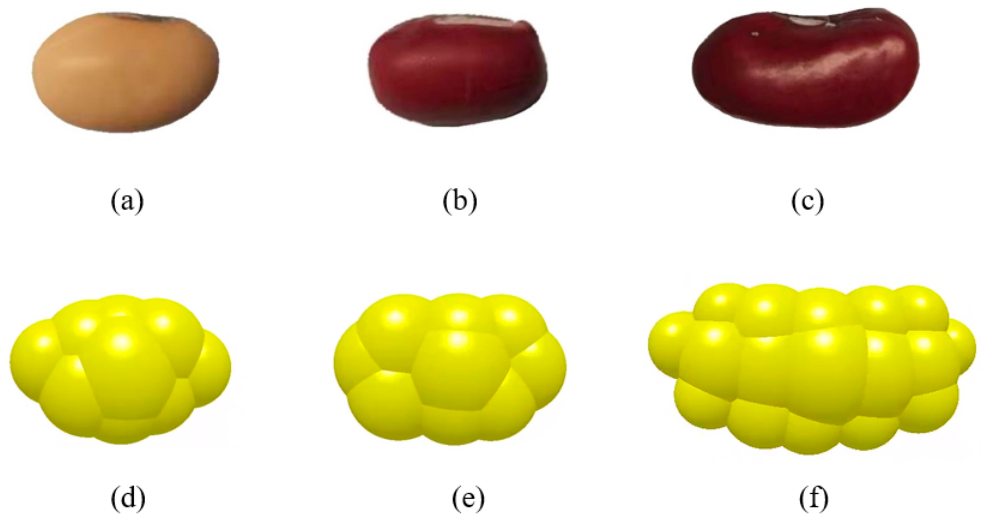
Figure 4.
Soil particle models with different filling spheres in the simulation: (a) globe with a sphere; (b) cylinder with two spheres; (c) cylinder with three spheres; (d) cone with three spheres; (e) pie-shaped with four spheres; and (f) pyramid with four spheres.
Figure 4.
Soil particle models with different filling spheres in the simulation: (a) globe with a sphere; (b) cylinder with two spheres; (c) cylinder with three spheres; (d) cone with three spheres; (e) pie-shaped with four spheres; and (f) pyramid with four spheres.
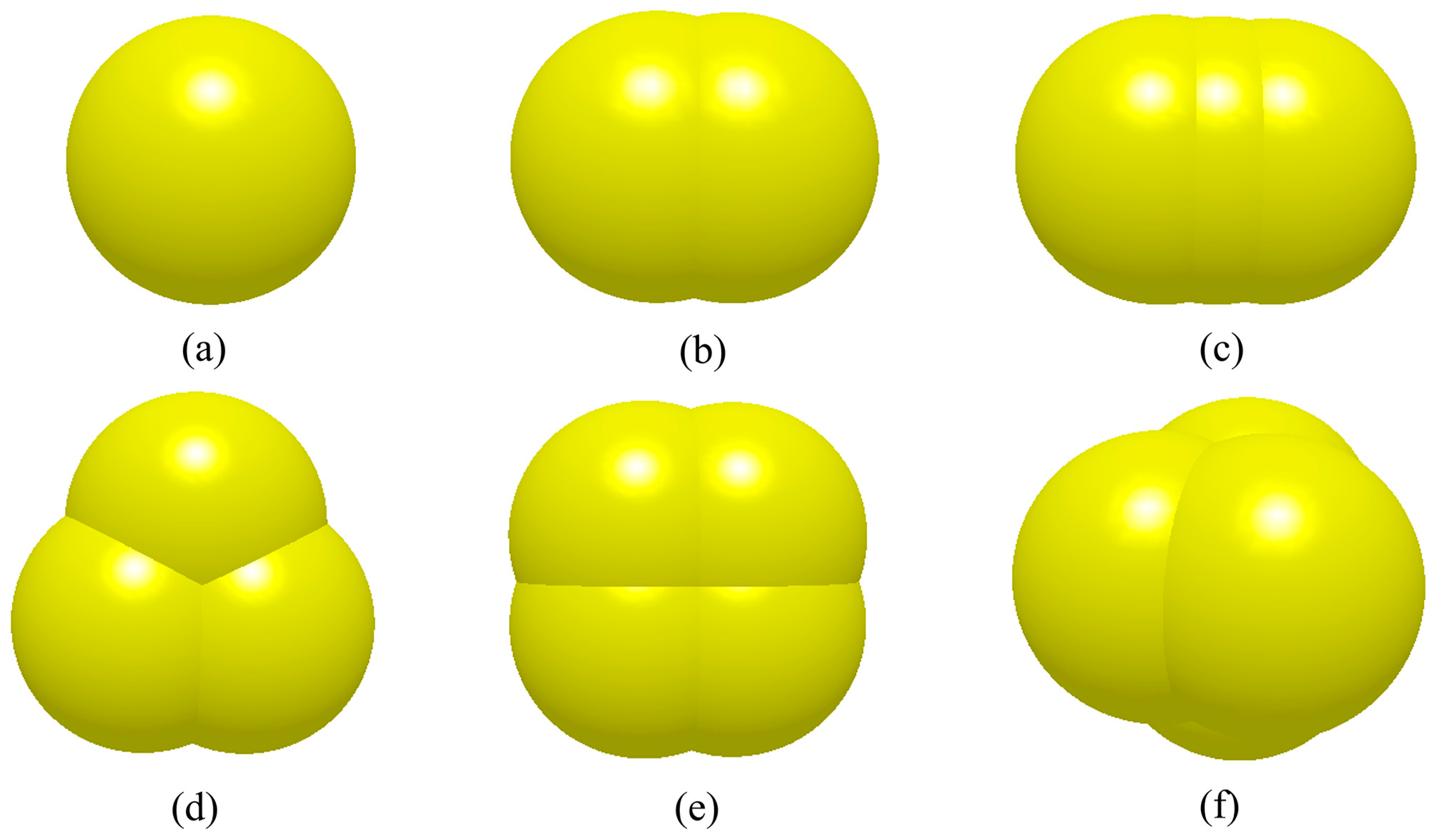
Figure 5.
ZJ-type fully automatic four-link direct shearing machine.

Figure 6.
Results of the direct shear test: (a) shearing displacement vs. shearing stress; (b) relationship curve between the normal loading and the shearing strength.
Figure 6.
Results of the direct shear test: (a) shearing displacement vs. shearing stress; (b) relationship curve between the normal loading and the shearing strength.

Figure 7.
Simulation of the direct shear test: (a) bonding key; (b) screenshot of the simulation test.
Figure 7.
Simulation of the direct shear test: (a) bonding key; (b) screenshot of the simulation test.
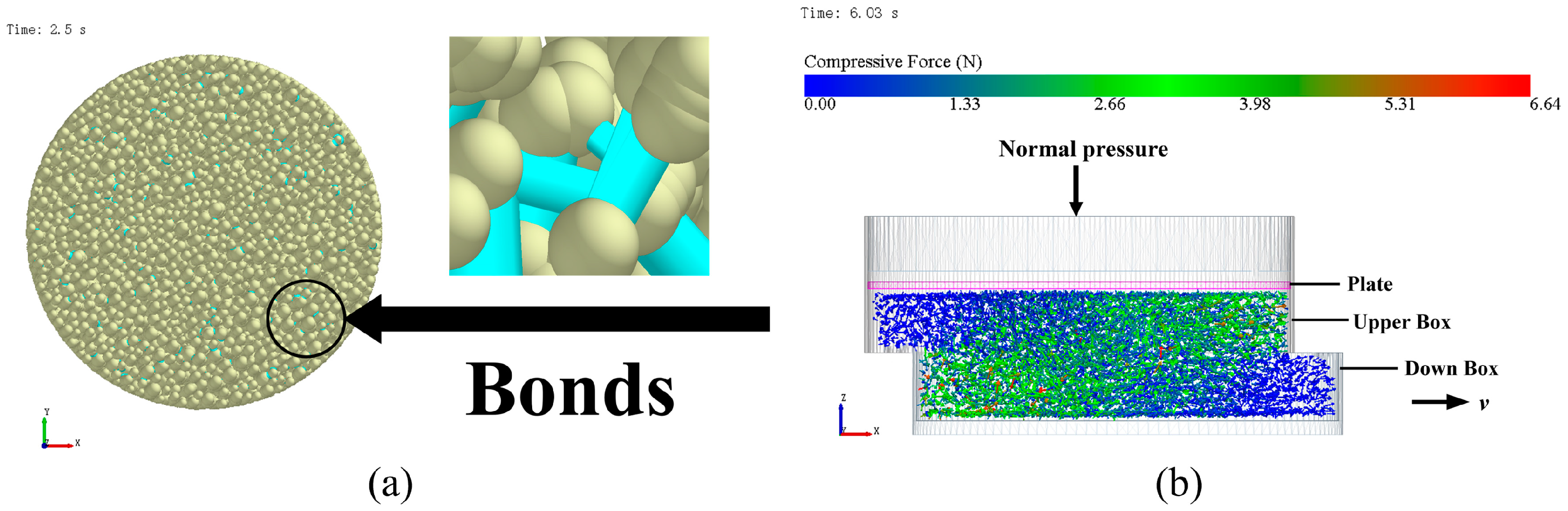
Figure 8.
Relationship curve between the actual and predicted values of the soil maximum shear strength.
Figure 8.
Relationship curve between the actual and predicted values of the soil maximum shear strength.

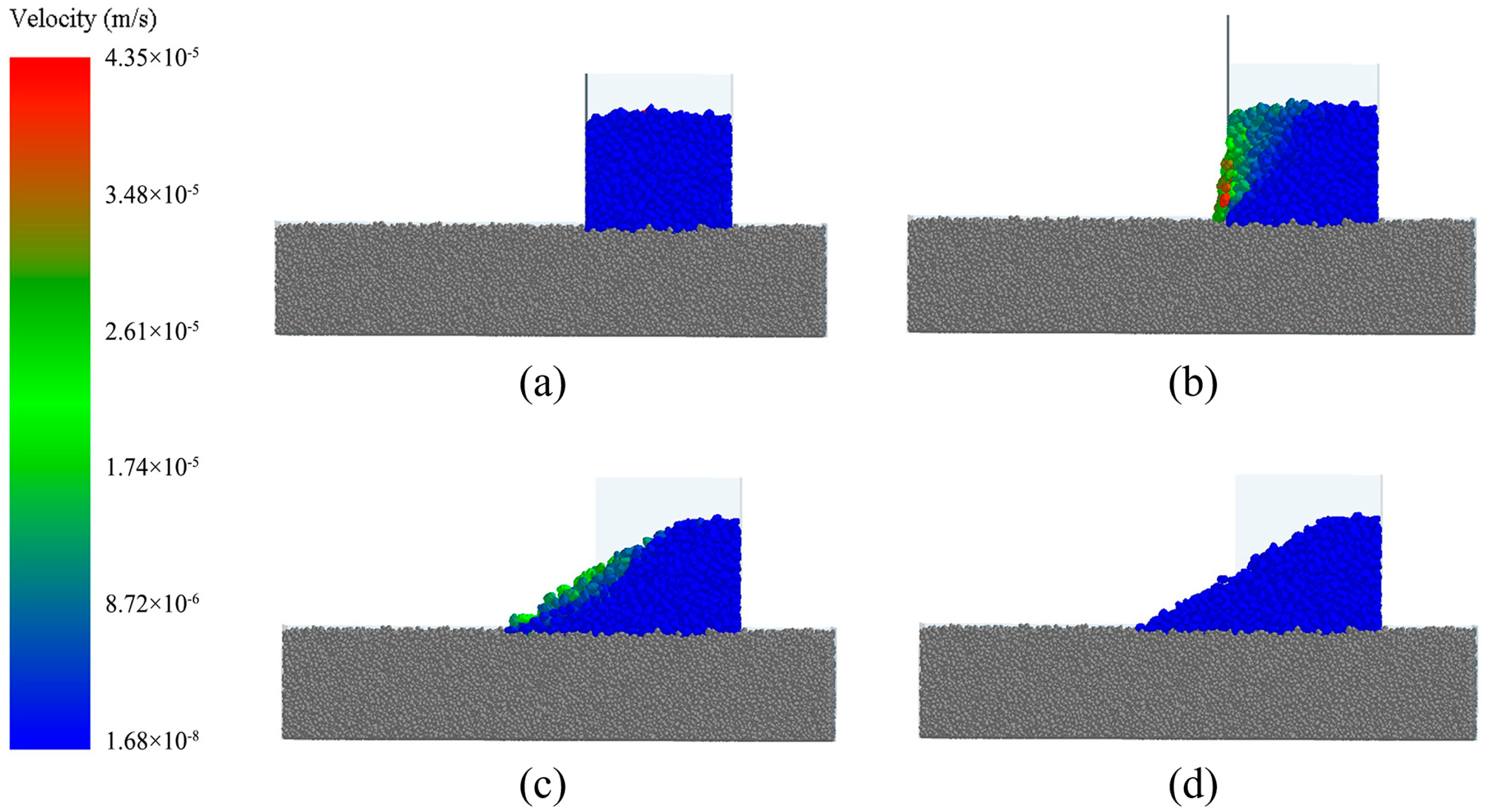
Figure 9.
Freefall test and simulation experiment for soybean plants: (a) freefall test; (b) simulation test, t = 0 s; (c) simulation test, t = 0.15 s; (d) simulation test, t = 0.2 s; and (e) simulation test, t = 0.27 s.
Figure 9.
Freefall test and simulation experiment for soybean plants: (a) freefall test; (b) simulation test, t = 0 s; (c) simulation test, t = 0.15 s; (d) simulation test, t = 0.2 s; and (e) simulation test, t = 0.27 s.

Figure 10.
Results for the coefficient of restitution of the three seeds for the experiment and simulation: (a) soybean seeds; (b) red bean seeds; (c) kidney bean seeds.
Figure 10.
Results for the coefficient of restitution of the three seeds for the experiment and simulation: (a) soybean seeds; (b) red bean seeds; (c) kidney bean seeds.

Figure 11.
Slope and simulation experiments for kidney bean: (a) slope experiment; (b) simulation test, t = 0 s; (c) simulation test, t = 2 s.
Figure 11.
Slope and simulation experiments for kidney bean: (a) slope experiment; (b) simulation test, t = 0 s; (c) simulation test, t = 2 s.

Figure 12.
Experimental and simulation test results for the static friction coefficient of the three seeds: (a) soybean seeds; (b) red bean seeds; (c) kidney bean seeds.
Figure 12.
Experimental and simulation test results for the static friction coefficient of the three seeds: (a) soybean seeds; (b) red bean seeds; (c) kidney bean seeds.

Figure 13.
Slope rolling and simulation experiments for red beans: (a) slope rolling experiment; (b) simulation test, t = 0 s; (c) simulation test, t = 4 s.
Figure 13.
Slope rolling and simulation experiments for red beans: (a) slope rolling experiment; (b) simulation test, t = 0 s; (c) simulation test, t = 4 s.

Figure 14.
Experimental and simulation test results for the rolling friction coefficient of the three seeds: (a) soybean seeds; (b) red bean seeds; (c) kidney bean seeds.
Figure 14.
Experimental and simulation test results for the rolling friction coefficient of the three seeds: (a) soybean seeds; (b) red bean seeds; (c) kidney bean seeds.

Figure 15.
Seed–soil piling test: (a) soybean seeds/soil; (b) red bean seeds/soil; (c) kidney bean seeds/soil.
Figure 15.
Seed–soil piling test: (a) soybean seeds/soil; (b) red bean seeds/soil; (c) kidney bean seeds/soil.
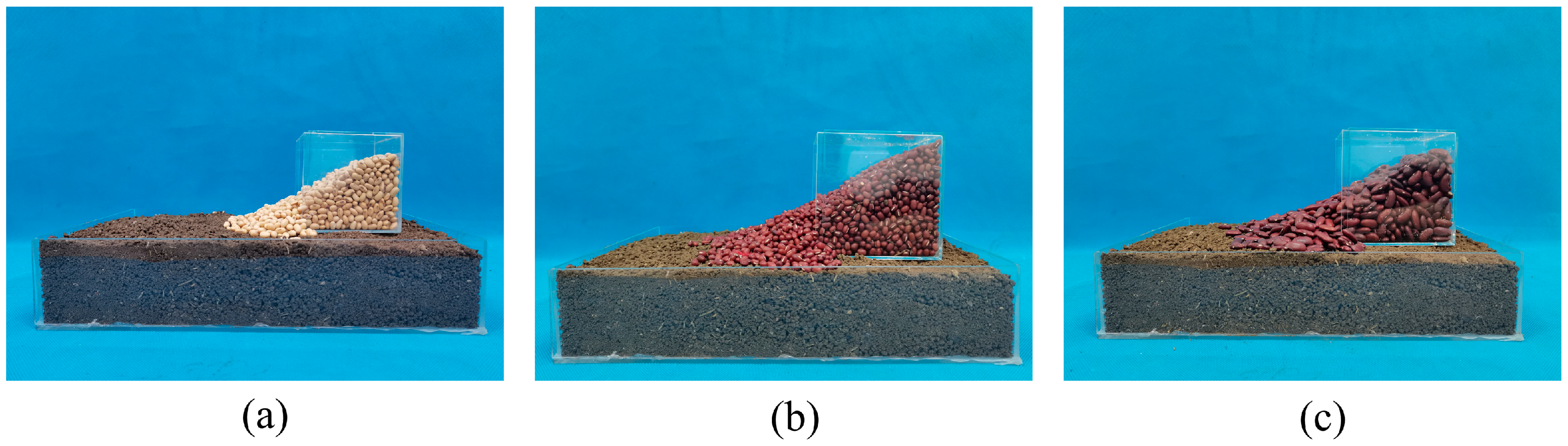
Figure 16.
Soybean seed–soil piling test at different times using the 9-sphere model: (a) t = 3.5 s; (b) t = 4 s; (c) t = 4.5 s; (d) t = 5 s.
Figure 16.
Soybean seed–soil piling test at different times using the 9-sphere model: (a) t = 3.5 s; (b) t = 4 s; (c) t = 4.5 s; (d) t = 5 s.

Figure 17.
Comparisons of the seed–soil piling test results.


Table 1.
Triaxial size, sphericity rate, and density of 100 seeds of each type with a certain moisture content.
Table 1.
Triaxial size, sphericity rate, and density of 100 seeds of each type with a certain moisture content.
| Seed Name | MC/ % | L/ mm | W/ mm | T/ mm | S | SD | Sphericity/ % | Density/ kg/m3 |
|---|---|---|---|---|---|---|---|---|
| Soybean | 14.77 | 8.38 | 5.48 | 4.48 | 1.5347 | 0.1293 | 70.49 | 1370 |
| Red bean | 18.50 | 7.54 | 5.24 | 4.87 | 1.4418 | 0.0891 | 76.55 | 1300 |
| Kidney bean | 13.78 | 16.41 | 7.93 | 5.69 | 2.0735 | 0.1125 | 55.14 | 1330 |
MC—moisture content; L—length; W—width; T—thickness; S = L/W; SD—standard deviation of L/W.
Table 2.
Arrangement and results of the path of steepest ascent method.
| No. | 1 | 2 | 3 | 4 | 5 |
|---|---|---|---|---|---|
| JKR surface energy (J/m2) | 3.5 | 4.5 | 5.5 | 6.5 | 7.5 |
| Normal stiffness per unit area (N/m3) | 1 × 10⁶ | 2 × 10⁶ | 3 × 10⁶ | 4 × 10⁶ | 5 × 10⁶ |
| Shear stiffness per unit area (N/m3) | 7 × 10⁵ | 6 × 10⁵ | 5 × 10⁵ | 4 × 10⁵ | 3 × 10⁵ |
| Critical normal stress (Pa) | 1000 | 1800 | 2600 | 3400 | 4000 |
| Critical shear stress (Pa) | 4000 | 3400 | 2600 | 1800 | 1000 |
| Maximum shear strength (kPa) | 38.5 | 41.1 | 38.6 | 40.1 | 39.5 |
| Relative error | 9.6% | 3.5% | 9.4% | 5.9% | 7.3% |
Table 3.
Box‒Behnken test parameter levels.
| No. | Level | −1 | 0 | +1 |
|---|---|---|---|---|
| A | JKR surface energy (J/m2) | 3.5 | 4.5 | 5.5 |
| B | Normal stiffness per unit area (106 N/m3) | 1 | 2 | 3 |
| C | Shear stiffness per unit area (105 N/m3) | 7 | 6 | 5 |
| D | Critical normal stress (Pa) | 1000 | 1800 | 2600 |
| E | Critical shear stress (Pa) | 4000 | 3400 | 2600 |
Table 4.
Box‒Behnken test design and results.
| No. | JKR Surface Energy (J/m2) | Normal Stiffness per Unit Area (106 N/m3) | Shear Stiffness per Unit Area (105 N/m3) | Critical Normal Stress (Pa) | Critical Shear Stress (Pa) | Maximum Shear Strength (kPa) |
|---|---|---|---|---|---|---|
| 1 | 3.5 | 1 | 6 | 1800 | 3300 | 38.6 |
| 2 | 5.5 | 1 | 6 | 1800 | 3300 | 39.7 |
| 3 | 3.5 | 3 | 6 | 1800 | 3300 | 40.2 |
| 4 | 5.5 | 3 | 6 | 1800 | 3300 | 40 |
| 5 | 4.5 | 2 | 5 | 1000 | 3300 | 39.1 |
| 6 | 4.5 | 2 | 7 | 1000 | 3300 | 39.6 |
| 7 | 4.5 | 2 | 5 | 2600 | 3300 | 38.3 |
| 8 | 4.5 | 2 | 7 | 2600 | 3300 | 38.4 |
| 9 | 4.5 | 1 | 6 | 1800 | 2600 | 38.3 |
| 10 | 4.5 | 3 | 6 | 1800 | 2600 | 40.2 |
| 11 | 4.5 | 1 | 6 | 1800 | 4000 | 39.8 |
| 12 | 4.5 | 3 | 6 | 1800 | 4000 | 38.7 |
| 13 | 3.5 | 2 | 5 | 1800 | 3300 | 38.4 |
| 14 | 5.5 | 2 | 5 | 1800 | 3300 | 39.1 |
| 15 | 3.5 | 2 | 7 | 1800 | 3300 | 38.7 |
| 16 | 5.5 | 2 | 7 | 1800 | 3300 | 38.2 |
| 17 | 4.5 | 2 | 6 | 1000 | 2600 | 39.9 |
| 18 | 4.5 | 2 | 6 | 2600 | 2600 | 38.9 |
| 19 | 4.5 | 2 | 6 | 1000 | 4000 | 38.9 |
| 20 | 4.5 | 2 | 6 | 2600 | 4000 | 39.3 |
| 21 | 4.5 | 1 | 5 | 1800 | 3300 | 39.1 |
| 22 | 4.5 | 3 | 5 | 1800 | 3300 | 39.4 |
| 23 | 4.5 | 1 | 7 | 1800 | 3300 | 37.5 |
| 24 | 4.5 | 3 | 7 | 1800 | 3300 | 38.9 |
| 25 | 3.5 | 2 | 6 | 1000 | 3300 | 39.5 |
| 26 | 5.5 | 2 | 6 | 1000 | 3300 | 39.3 |
| 27 | 3.5 | 2 | 6 | 2600 | 3300 | 37.9 |
| 28 | 5.5 | 2 | 6 | 2600 | 3300 | 40.2 |
| 29 | 4.5 | 2 | 5 | 1800 | 2600 | 38.2 |
| 30 | 4.5 | 2 | 7 | 1800 | 2600 | 38.2 |
| 31 | 4.5 | 2 | 5 | 1800 | 4000 | 38.1 |
| 32 | 4.5 | 2 | 7 | 1800 | 4000 | 38.4 |
| 33 | 3.5 | 2 | 6 | 1800 | 2600 | 39.2 |
| 34 | 5.5 | 2 | 6 | 1800 | 2600 | 39.3 |
| 35 | 3.5 | 2 | 6 | 1800 | 4000 | 38.3 |
| 36 | 5.5 | 2 | 6 | 1800 | 4000 | 39.8 |
| 37 | 4.5 | 1 | 6 | 1000 | 3300 | 40.9 |
| 38 | 4.5 | 3 | 6 | 1000 | 3300 | 39.2 |
| 39 | 4.5 | 1 | 6 | 2600 | 3300 | 39.1 |
| 40 | 4.5 | 3 | 6 | 2600 | 3300 | 40.1 |
| 41 | 4.5 | 2 | 6 | 1800 | 3300 | 41.8 |
| 42 | 4.5 | 2 | 6 | 1800 | 3300 | 42.2 |
| 43 | 4.5 | 2 | 6 | 1800 | 3300 | 42.8 |
| 44 | 4.5 | 2 | 6 | 1800 | 3300 | 42.6 |
| 45 | 4.5 | 2 | 6 | 1800 | 3300 | 42.4 |
| 46 | 4.5 | 2 | 6 | 1800 | 3300 | 42.1 |
Table 5.
Significance analysis of the factors in the BB test.
| Source | Sum of Squares | df | Mean Square | F-Value | p-Value | |
|---|---|---|---|---|---|---|
| Model | 74.15 | 20 | 3.71 | 22.12 | <0.0001 | Significant |
| A | 1.44 | 1 | 1.44 | 8.59 | 0.0071 | |
| B | 0.8556 | 1 | 0.8556 | 5.11 | 0.0328 | |
| C | 0.2025 | 1 | 0.2025 | 1.21 | 0.2822 | |
| D | 1.10 | 1 | 1.10 | 6.58 | 0.0167 | |
| E | 0.0506 | 1 | 0.0506 | 0.3021 | 0.5875 | |
| AB | 0.4225 | 1 | 0.4225 | 2.52 | 0.1249 | |
| AC | 0.3600 | 1 | 0.3600 | 2.15 | 0.1552 | |
| AD | 1.56 | 1 | 1.56 | 9.32 | 0.0053 | |
| AE | 0.4900 | 1 | 0.4900 | 2.92 | 0.0997 | |
| BC | 0.3025 | 1 | 0.3025 | 1.80 | 0.1912 | |
| BD | 1.82 | 1 | 1.82 | 10.87 | 0.0029 | |
| BE | 2.25 | 1 | 2.25 | 13.42 | 0.0012 | |
| CD | 0.0400 | 1 | 0.0400 | 0.2387 | 0.6294 | |
| CE | 0.0225 | 1 | 0.0225 | 0.1342 | 0.7172 | |
| DE | 0.4900 | 1 | 0.4900 | 2.92 | 0.0997 | |
| A2 | 20.13 | 1 | 20.13 | 120.11 | <0.0001 | |
| B2 | 13.50 | 1 | 13.5 | 80.55 | <0.0001 | |
| C2 | 44.26 | 1 | 44.26 | 264.10 | <0.0001 | |
| D2 | 15.56 | 1 | 15.56 | 92.86 | <0.0001 | |
| E2 | 27.05 | 1 | 27.05 | 161.37 | <0.0001 | |
| Residual | 4.19 | 25 | 0.1676 | |||
| Lack of fit | 3.54 | 20 | 0.1771 | 1.37 | 0.3923 | Not significant |
| Pure error | 0.6483 | 5 | 0.1297 | |||
| Cor total | 78.34 | 45 |
Table 6.
Parameters used in the simulations.
| Materials | Parameters | Values | Source |
|---|---|---|---|
| Soils | Density/kg·m−3 | 1950 | Measured |
| Shear modulus/Pa | 2.73 × 10⁶ | Reference [27] previous work | |
| Poisson’s ratio | 0.2 | Reference [27] previous work | |
| Coefficient of restitution | 0.3 | Reference [27] previous work | |
| Static friction coefficient | 0.5 | Reference [27] previous work | |
| Coefficient of rolling friction | 0.03 | Reference [27] previous work | |
| Surface energy/J·m−2 | 4.436 | Calibrated (direct shear test) | |
| Normal stiffness per unit area (106 N/m3) | 2.86 | Calibrated (direct shear test) | |
| Shear stiffness per unit area (105 N/m3) | 5.54 | Calibrated (direct shear test) | |
| Critical normal stress (Pa) | 1833 | Calibrated (direct shear test) | |
| Critical shear stress (Pa) | 3332 | Calibrated (direct shear test) | |
| Kidney beans | Density/kg·m−3 | 1340 | Measured |
| Shear modulus/Pa | 4.535 × 10⁷ | Measured | |
| Poisson’s ratio | 0.4 | Reference [26] | |
| Coefficient of restitution | 0.45 | Measured | |
| Static friction coefficient | 0.48 | Measured | |
| Coefficient of rolling friction | 0 | Measured | |
| Coefficient of restitution with soil | 0.25 | Calibrated (single factor experiments) | |
| Static friction coefficient with soil | 0.5 | Calibrated (single factor experiments) | |
| Coefficient of rolling friction with soil | 0.14 | Calibrated (single factor experiments) | |
| Red beans | Density/kg·m−3 | 1300 | Measured |
| Shear modulus/Pa | 1.414 × 10⁷ | Measured | |
| Poisson’s ratio | 0.4 | Reference [26] | |
| Coefficient of restitution | 0.45 | Measured | |
| Static friction coefficient | 0.48 | Measured | |
| Coefficient of rolling friction | 0 | Measured | |
| Coefficient of restitution with soil | 0.25 | Calibrated (single factor experiments) | |
| Static friction coefficient with soil | 0.65 | Calibrated (single factor experiments) | |
| Coefficient of rolling friction with soil | 0.14 | Calibrated (single factor experiments) | |
| Soybean | Density/kg·m−3 | 1370 | Measured |
| Shear modulus/Pa | 1.768 × 10⁷ | Measured | |
| Poisson’s ratio | 0.4 | Reference [26] | |
| Coefficient of restitution | 0.45 | Measured | |
| Static friction coefficient | 0.48 | Measured | |
| Coefficient of rolling friction | 0.04 | Measured | |
| Coefficient of restitution with soil | 0.25 | Calibrated (single factor experiments) | |
| Static friction coefficient with soil | 0.6 | Calibrated (single factor experiments) | |
| Coefficient of rolling friction with soil | 0.10 | Calibrated (single factor experiments) |
Table 7.
Seed–soil piling test results.
| Seed | Stacking Angle θ/° | SD/° |
|---|---|---|
| Soybean | 29.12 | 0.9945 |
| Red bean | 26.57 | 0.2354 |
| Kidney bean | 27.09 | 0.5801 |
Disclaimer/Publisher’s Note: The statements, opinions and data contained in all publications are solely those of the individual author(s) and contributor(s) and not of MDPI and/or the editor(s). MDPI and/or the editor(s) disclaim responsibility for any injury to people or property resulting from any ideas, methods, instructions or products referred to in the content. |
© 2024 by the authors. Licensee MDPI, Basel, Switzerland. This article is an open access article distributed under the terms and conditions of the Creative Commons Attribution (CC BY) license (https://creativecommons.org/licenses/by/4.0/).
Share and Cite
MDPI and ACS Style
Xu, T.; Fu, H.; Yu, J.; Li, C.; Wang, J.; Zhang, R. Determination of Ellipsoidal Seed–Soil Interaction Parameters for DEM Simulation. Agriculture 2024, 14, 376. https://doi.org/10.3390/agriculture14030376
AMA Style
Xu T, Fu H, Yu J, Li C, Wang J, Zhang R. Determination of Ellipsoidal Seed–Soil Interaction Parameters for DEM Simulation. Agriculture. 2024; 14(3):376. https://doi.org/10.3390/agriculture14030376
Chicago/Turabian StyleXu, Tianyue, Hao Fu, Jianqun Yu, Chunrong Li, Jingli Wang, and Ruxin Zhang. 2024. "Determination of Ellipsoidal Seed–Soil Interaction Parameters for DEM Simulation" Agriculture 14, no. 3: 376. https://doi.org/10.3390/agriculture14030376
Note that from the first issue of 2016, this journal uses article numbers instead of page numbers. See further details here.