Analysis and Structural Optimization Test on the Collision Mechanical Model of Blade Jun-Cao Grinding Hammer

1
College of Agriculture Engineering, Shanxi Agricultural University, Jinzhong 041399, China
2
College of Mechanical and Electrical Engineering, Fujian Agriculture and Forestry University, Fuzhou 350002, China
*
Author to whom correspondence should be addressed.
Agriculture 2024, 14(3), 492; https://doi.org/10.3390/agriculture14030492
Submission received: 28 February 2024
/
Revised: 12 March 2024
/
Accepted: 13 March 2024
/
Published: 18 March 2024
(This article belongs to the Section Agricultural Technology)
Abstract
:Aiming at the problems found in grinding Jun-Cao, such as poor grinding effect and high grinding power of mill, this study proposes a blade Jun-Cao grinding hammer based on the traditional hammer mill. With dynamics model analysis, it had better performance than a traditional hammer. By simulating the operation process in the DEM, forces on Jun-Cao and their motions were analyzed. By optimizing the structural parameters of the hammer blade based on multiobjective optimization using the genetic algorithm, an optimal solution set was obtained as a reference for practical production. Meanwhile, a bench test was designed to compare the traditional rectangular hammer with the new blade hammer regarding the operation effect. The result proved the following: (1) cutting edge length, cutting edge thickness and hammer thickness had a significant influence on the grinding effect and grinding power; (2) a total of 22 optimal solution sets were obtained, based on which the blade hammer with a cutting edge length of 45 mm, a cutting edge thickness of 3 mm and a hammer thickness of 7 mm was finally selected in the bench test; (3) the bench test proved that the blade hammer was generally superior to the traditional rectangular hammer with the output per kilowatt-hour having been improved by 13.55% on average.
1. Introduction
As a novel energy plant, Jun-Cao can survive easily with low requirements on growing conditions [1]. The ground Jun-Cao can serve as a base for edible mushrooms. With a shorter growth cycle and higher yield than trees, the reasonable use of Jun-Cao for growing edible mushrooms can save vast amounts of timber and solve the “contradiction between mushroom and forest” [2,3] caused by mushroom cultivation. As a base for edible mushrooms, when Jun-Cao fails to be grounded evenly, it will directly affect the growth conditions of fungi. However, high energy consumption and low grinding efficiency of mill have become the key factors hindering the promotion and development of the Jun-Cao industry.
Now, as one of the most widely applied machines, the hammer mill has significantly affected the grinding of Jun-Cao in terms of the structure, quantity and motion state of hammer blades [4]. By comparing the laws affecting the working efficiency of mill and the specific energy consumption through the T-shaped hammer blade and the traditional hammer, Bochat et al. [5] found that such a hammer blade could improve the screening efficiency after the grinding of materials by breaking the circulation layer formed during the rotation of materials after the comparison. With the development of computer field and various optimization algorithms, optimization algorithms are gradually being introduced into various fields, including structural design. Paraschiv et al. [6] improved the hammer of hammer mill from several aspects and obtained the optimal blade structure. Tekgüler et al. [7] studied the influence of slotted screen and round-hole screen on the working performance of mills. Evans et al. [8] studied the influence of mesh diameter and blade velocity on the grinding effect, revealing that there was a slightly significant linear relationship between mesh diameter and blade velocity with the geometric mean particle size and geometric standard deviation. Djordjevic et al. [9] suggested the use of DEM technology to analyze the grinding operation. Afterwards, Ghodki et al. [10] simulated the state of seeds in a mill and analyzed the grinding effect based on the DEM. Chen et al. [11] designed a straw fiber crusher, and explored crusher parameters and working effect with central composite experiments by DEM simulation. Egorov et al. [12] revealed that a rotary stirring machine could improve particle distribution uniformity in their research. Cotabarren et al. [13] proposed a developed model to predict the dynamic behavior of a hammer mill, which provides research based on milling performance and could predict confidence operating point. Vanarase et al. [14] compared the conical grinder with hammer mill regarding the grinding effect, revealing that the conical grinder could achieve a better grinding effect while a hammer mill would discharge the materials that were not completely ground. Similarly, Vukmirovic et al. [15] compared the effects through two different grinding methods, and their result showed that materials were more uniform in size after grinding by roller mill but generally had a larger diameter; this was quite contrary for the hammer mill. Wang et al. [16] designed a pointed hammer and a bevel-faced hammer. The DEM analysis revealed that using the pointed hammerhead would improve the productivity of hammerhead mill. However, the adoption of beveled hammerhead would reduce the power consumption per ton and the temperature rise of feeding materials. At present, the research on biomass crushing is related to the fact that the research object is quite different from Jun-Cao. On the other hand, the research is focused on the hammer structure [17,18,19,20,21], model prediction [22], flow field analysis [23] and properties analysis [24,25,26], and the analysis of the force model in the crushing process is relatively vague.
In this paper, starting from the structure of hammer blade, a selective analysis was made on the mechanical model between hammer blade and Jun-Cao. By designing a brand-new blade Jun-Cao hammer, a discrete element model was built in the simulation test to analyze the influence of the structural parameters of blade hammer on the operation effect. Also, a test bench was constructed to verify the feasibility of the blade hammer.
2. Materials and Methods
2.1. Design of Hammer Blade
In this paper, a hammer blade was designed based on the traditional rectangular hammer. Reshaping the hammer at both ends would perfect the pressure angle of hammer to increase the impact efficiency. The structure of hammer blade is shown in Figure 1, where the reduction in hammer thickness at the center could reinforce the impact stress. In order to guarantee rotor balancing for replacing hammer blades in the future, symmetrical mounting hammer blades were selected in this paper. Compared with the traditional rectangular hammer, our blade hammer had higher stress on the blade edge to cut and break Jun-Cao stalks. Meanwhile, it would crush Jun-Cao stalks due to the shape of the hammer blade at both ends, which at the same time would result in a radial velocity on stalks to allow them to be ground more completely.
Figure 2a shows the mechanical model for the contact between material and traditional hammer. Assuming that forces are constant during the contact between hammer blade and materials, according to the law of conservation of momentum, forces on materials could be as follows:
where m represents material mass (kg), represents the velocity of material (m/s) before the contacting, indicates the velocity of material (m/s) after the contacting and t is the time of contact.
The rotation speed of hammer mill was stable during the operation; then, forces on materials could be as follows:
where is the rotate speed of hammer blade (rad/s), r is the distance (mm) from the hammer blade–material touch point to the center of gyration, B is the hammer thickness (mm) at the touch point and p is the width of the touch point (mm).
Formula (2) reveals that compared with the traditional rectangular hammer, our brand-new hammer is thinner at the touch point to suffer more stress when the materials come into contact with the cutting edge of the hammer blade.
Figure 2b shows the mechanical model for the contact between material and our new hammer. According to the geometrical relationship, the contact distances of these two hammer blades are separate, as shown below:
where is the contact distance (mm) of the traditional hammer, is the contact distance (mm) of our blade hammer and h is the contact height (mm).
The contrast between Formulas (3) and (4) reveals that the contact distance of our new hammer was longer than that of the traditional hammer when each hammerhead came into contact with materials at the same contact height of h. Hence, according to Formula (2), compared with the traditional hammer, blade hammer put more stress on the materials so that they could be ground more easily.
Similarly, according to the geometrical relationship, when materials came into contact with each hammerhead, the pressure angle of material was separate as follows:
As an included angle between velocity and stress, the reduced pressure angle represented higher efficiency in joining forces. The contrast between Formulas (5) and (6) revealed that blade hammer would achieve higher grinding efficiency by adjusting the pressure angle of materials after the change of the included angle .
2.2. Simulation Environment
In this paper, EDEM-based simulation was used to analyze the material grinding process through hammer blade. As shown in Figure 3, the simulated hammer blade and box were converted into the igs format and imported into the EDEM after they had been plotted in SolidWorks. The hammer blade was set with a Poisson’s ratio of 0.25 for the material, a density of 7800 kg/m3 and a shear modulus of 7000 MPa. Then, the Whole and Fraction particles were separately built to simulate Jun-Cao stalks through bonds. The Whole particles were 10 mm in diameter, while the Fraction particles had a diameter of 0.5 mm. Both particles had the same constitutive parameters with a Poisson’s ratio of 0.4 for the particles, a particle density of 1060 kg/m2 and a shear modulus of 170 Mpa. Both particles have the same coefficients of contact and parameters of bonds. Table 1 shows the coefficients of the contact between particles, and Table 2 shows the parameters of bonds.
Figure 4 shows the process of acquiring the particle model. Firstly, a cylindrical particle factory with a length of 180 mm and a diameter of 40 mm were built with the model set to be Physical. Then, a Jun-Cao stalk model with a length of 60 mm, an outer diameter of 20 mm and an inner diameter of 13 mm was inserted into the cylinder, and this model was set to be Virtual. The Whole and Fraction particles were generated in this particle factory without the introduction of bonds temporarily. After the whole cylinder was filled with particles, we returned to the setting interface to revise the external cylindrical model to be Virtual and set the Jun-Cao stalk model to be Physical. Meanwhile, by replacing the Whole particles with Fraction particles through particle replacement, redundant particles would fall down due to the gravity. Finally, with the introduction of bonds into the remaining particles in the Jun-Cao stalk model and the saving of Material block, the Jun-Cao stalk model was then constructed, where there were a total of 20,858 particles and 113,088 bonds in a single Jun-Cao stalk.
2.3. Experimental Method
In order to explore the influence of the cutting edge thickness of blade hammer on the grinding effect, the cutting edge length, cutting edge thickness and hammer thickness were selected as the factors, and the number of broken bonds calculated during the post-processing in EDEM was taken as the index to evaluate the grinding effect. Then, the average torque of hammer blade was calculated and the mean operating power obtained according to Formula (7) was considered as the index of grinding power for designing CCD test. Table 3 is the factor level table.
After the experiment began, at Material block was set to feed in 10 Jun-Cao stalks from the feeding inlet; at the same time, hammers began to rotate at a speed of 2800 r/min. In order to simulate the force induced by the airflow of mill, Jun-Cao stalks were accelerated by 2 m/s in the negative direction of z-axis so that materials could be ground when they moved into the grinding zone. The time step was 8 × 10⁻⁷ s and the simulation lasted for totally 1 s. The target save interval was 0.05 s and the meshing size was 1.5 mm. Furthermore, in order to explore the motion of Jun-Cao particles during the operation of mill, the target save interval was set to be 0.01 s for an additional experiment, where the above three factors were set at zero level.
After the test, the average torque and the number of bonding key failures of the hammer during the operation are exported in the post-processing interface. The operation power is calculated by the average torque, and the operation volume is measured by the number of bonding key failures.
2.4. Bench Test Instrument
The bench test was conducted in the engineering training center, College of Mechanical and Electronic Engineering, Fujian Agriculture and Forestry University. The following instruments were mainly used in the experiment, including the prototype of blade Jun-Cao grinding mill, blade hammer, rectangular hammer, three-phase asynchronous motor, frequency converter, three-phase four-wire electronic watt-hour meter, electronic scale and stop watch, etc. Figure 5 shows the test environment.
After the bench test starts, connect the motor power and adjust the motor speed to 2800 r/min. After the motor speed is stable, feed the Jun-Cao continuously from the inlet. After the Jun-Cao is smashed by the hammer, it will be discharged from the outlet by the airflow field inside the crusher. Weigh the discharged Jun-Cao particles and record them, and use the power meter to record the power consumed by the operation.
3. Results
3.1. Analysis on the Grinding Effect of Hammer Blade
Figure 6 shows the material velocity distribution in 0.01 s–0.04 s after the mill began to work. At 0.01 s, the forepart of the Jun-Cao stalk was smashed and ground by the hammer after it entered the operating region. After the grinding, Jun-Cao particles moved rapidly and dispersed but the rear part of Jun-Cao remained unchanged. At 0.02 s, particles of the ground Jun-Cao scattered on the inner wall and at the same time, some material blocks that failed to be smashed completely slowly separated from the Jun-Cao stalk. At 0.03 s, more material blocks that failed to be ground completely arose on the Jun-Cao stalk and some Jun-Cao particles gradually began to move slower. At 0.04 s, when the whole Jun-Cao stalk entered the grinding region, more and more material blocks that failed to be smashed completely arose and the Jun-Cao particles moved even more slowly as a whole.
Figure 7 shows the velocity distribution of Jun-Cao particles within the mill in the period of 0.1 s–0.4 s. At 0.1 s, the velocity of Jun-Cao particles became relatively stable. But in the grinding region, there were still lots of material blocks in large size failing to be crushed completely. At 0.2 s, the velocity of the whole material was further reduced and some material blocks that failed to be ground completely became smaller in size due to the impact of the hammer. At 0.3 s, the velocity of material gradually tended to be stable and the material blocks became even smaller in size due to the smashing. At 0.4 s, the grinding operation was basically completed, but some material blocks still failed to be ground. The reason might lie in the wide gap between the hammer and the inner wall caused by the insufficient length of the hammer.
Figure 8 shows the bond breakages in Jun-Cao stalk. There were totally 1,103,422 bonds after the formation of Jun-Cao stalk. Then, the number of unbroken bonds dwindled down while the number of broken bonds increased gradually. In the period of 0 s–0.1 s, numerous bonds in Jun-Cao stalks were damaged with the number of broken bonds rising from 0 to 600 thousand. In fact, more than half of the bonds were broken in this period. In the period of 0.1–0.6 s, bonds in the Jun-Cao stalks continued to be damaged at a certain rate with the number of broken bonds rising from 600 thousand to 750 thousand. After 0.6 s, the grinding efficiency became rather poor with a very small number of bonds having been broken. At this moment, the mill was in a stable state.
3.2. Regression Analysis
Table 4 shows the simulation result, and Table 5 shows the quadratic regression analysis on the number of broken bonds. The p value of the regression model less than 0.0001 indicates the significance of the regression model. The lack of fit higher than 0.1 reveals that error was not significant. Hence, the test result was good and reliable. The p value of the single factors—A, B, C—and the quadratic terms—A2, B2—was lower than 0.05, this revels that they had an extremely significant influence on the number of broken bonds. The p value of the interaction term, AB higher than 0.05 but lower than 0.1, reflects its significant influence on the number of broken bonds. However, as the p value of the interaction terms BC, AC and the quadratic term C2 was higher than 0.1, it proves that they did not have a significant influence on the bonds. According to the regression analysis, the quadratic regression equation is provided as below:
Table 6 shows the quadratic regression analysis result for the average power of hammer blade. As shown in the table, the p value of the regression model was lower than 0.0001, indicating the significance of the model. The lack of fit was higher than 0.1, reflecting that the error was not significant. Hence, the test result was satisfactory and reliable. The p value of the single factors, A, B, C; the interaction term AB; and the quadratic term A2, B2 less than 0.05 reveals their extremely significant influence on mean power. Further, the p value of the interaction term BC being higher than 0.05 but lower than 0.1 indicates its significant influence on mean power. Meanwhile, the p value of the interaction term AC and the quadratic term C2 was higher than 0.1, reflecting that their influence on mean power was not significant. According to the regression analysis, the quadratic regression equation is provided as below:
3.3. Response Surface Analysis
As indicated in Figure 9, the response surface between A (the cutting edge length), B (the cutting edge thickness) and C (the hammer thickness) with Y (the number of broken bonds) was plotted according to the quadratic regression equation for the number of broken bonds. Figure 9a shows the interaction between A and B with the number of broken bonds when the hammer thickness C was 5 mm. As shown in the figure, when B remained unchanged, the number of broken bonds would rise linearly with the increase in A from 25 mm to 45 mm. However, when A remained unchanged, the number of broken bonds would drop linearly with the increase in B from 1 mm to 3 mm. At least 650,000 bonds were damaged when A was 25 mm and B was 3 mm. But when A was 45 mm and B was 1 mm, the number of broken bonds was around 920,000 to the maximum. Figure 9b shows the interaction between A and C with the number of broken bonds when B was 2 mm. As indicated in the figure, when C remained unchanged, the number of broken bonds went up linearly with the increase in A from 25 mm to 45 mm. However, when A remained unchanged, with the increase in C from 3 mm to 7 mm, there was a slightly linear decline in the number of broken bonds. When A was 25 mm and C was 7 mm, the number of broken bonds was roughly 680,000 to the minimum. But when A was 45 mm and C was 3 mm, the number of broken bonds was up to be around 880,000 maximally. Figure 9c shows the interaction between B and C with the number of broken bonds when A was always 35 mm. As shown in the figure, when C remained unchanged, the number of broken bonds reduced linearly with the increase in B from 1 mm to 3 mm. When B remained unchanged, with the increase in C from 3 mm to 5 mm, there was a slightly linear decline in the number of broken bonds. When B was 3 mm and C was 7 mm, the number of broken bonds was 700,000 to the minimum. When B was 1 mm and C was 3 mm, the number of broken bonds was up to around 850,000 maximally.
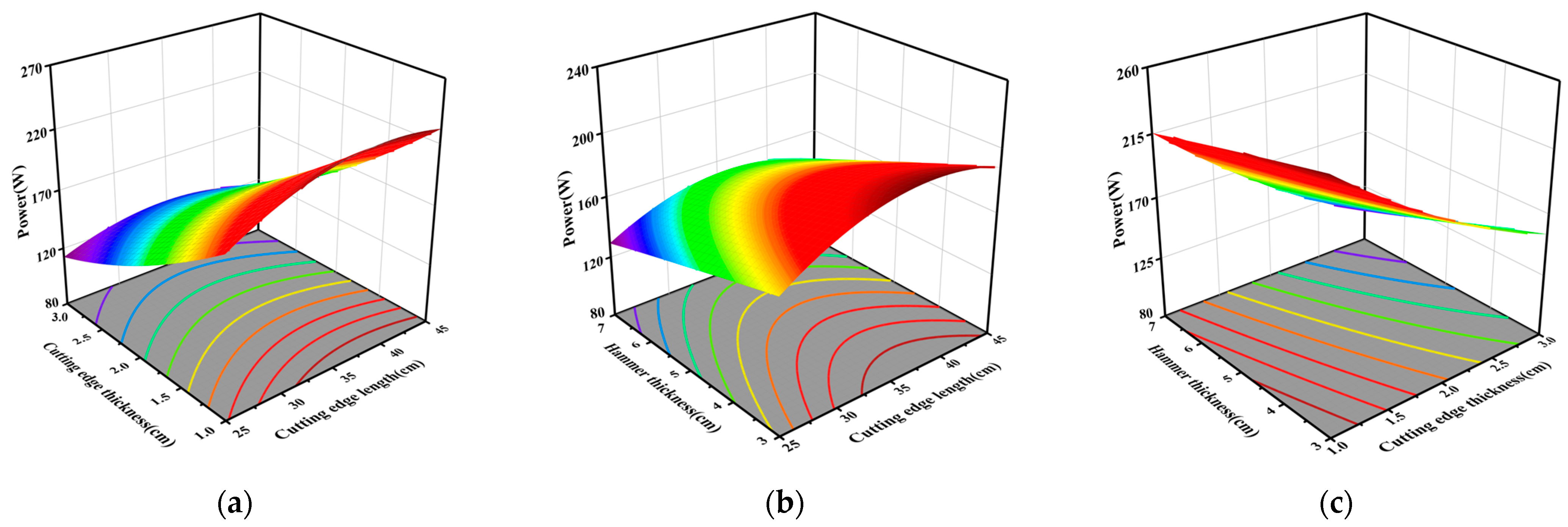
As shown in Figure 10, the response surface between A (the cutting edge length), B (the cutting edge thickness) and C (the hammer thickness) with P (the mean power) is plotted according to the quadratic regression equation for mean power. Figure 10a shows the interaction between A and B with the mean power P when C was 5 mm. As indicated in the figure, when B remained unchanged, the mean power increased and then declined with the increase in A from 25 mm to 45 mm. When A remained unchanged, the mean power P showed a downward trend with the increase in B from 1 mm to 3 mm. When A was 25 mm and B was 3 mm, P (the mean power) reached the minimum value of about 110 W. However, it reached its maximum of around 240 W when A was about 38 mm and B was 1 mm. Figure 10b shows the interaction between A and C with the mean power P when B was 2 mm. As shown in the figure, when C remained unchanged, P first showed an upward trend and then declined with the increase in A from 25 mm to 45 mm. When A was kept unchanged, P showed a slightly downward trend with the increase in C from 3 mm to 7 mm. When A was 25 mm and C was 7 mm, P reached the minimum value of about 120 W. However, it reached its maximum of around 200 W when A was 37 mm and C was 3 mm. Figure 10c shows the interaction between B and C when A was 35 mm. As shown in the figure, when C was fixed, P showed a downward trend with the increase in B from 1 mm to 3 mm. In the case of B unchanged, P showed a small declining trend when C was increased from 3 mm to 7 mm. When B was 3 mm and C was 7 mm, P reached the minimum value of about 100 W; however, it reached a maximum of about 250 W when B was 1 mm and C was 3 mm.
3.4. Parameter Optimization
In practice production, it is generally required that highly efficient grinding be guaranteed with the control of grinding power. However, according to the above regression analysis, the improvement in grinding efficiency also meant the increase in mean power. In this paper, the multiobjective genetic algorithm in Matlab R2018b was used to optimize the parameters of hammer blade with the objective function and constraints provided as below:
3.5. Contrast Test
After the optimization and in order to compare the performance of our new hammer, a contrast test was conducted in this paper to compare the hammer with a cutting edge length of 45 mm, a cutting edge thickness of 3 mm and a hammer thickness of 7 mm with the traditional hammer. In the test, no-load operation was made on the mill at a rate of 2800 r/min through the frequency converter. After the stable operation of mill, Jun-Cao stalks were fed continuously and uniformly, and a total of 30 kg of materials were fed ground for 10 min. After the grinding in the mill, the crushed materials were weighted on an electronic scale and the number displayed on the watt-hour meter was recorded. The mill was separately installed with the new and traditional hammers in two tests. Other parameters remain unaltered. In each test, a total of five experiments were conducted to calculate the mean value. The experimental results are provided in Table 8 and Table 9.
In order to better evaluate the operation effects of the new and the traditional hammer blades, the output per Kilowatt-hour was selected as the evaluation index to test the working performance of the mill during the normal operation of the machine according to the Chinese standard [27] with the calculation method provided as below:
where G is the output per kilowatt-hour, kg/(kW·h); M is the operating mass in working hours, kg; and Q is the power consumption in working hours, kW·h.
Figure 12 shows the result of the contrast test. The five tests revealed that through the traditional rectangular hammer mill, the mean operating mass was 18.78 kg in 10 min with a standard deviation of 1.05, the average power consumption was 1.02 kW·h with a standard deviation of 0.08 and the average output per kilowatt-hour was 18.41 kg/(kW·h) with a standard deviation of 0.58. However, with our brand-new hammer, the mean operating mass was 20.49 kg with a standard deviation of 2.14, the average power consumption was 0.98 kW·h with a standard deviation of 0.08 and the average output per kilowatt-hour was 20.90 kg/(kW·h) with a standard deviation of 0.68. The results show that compared with the traditional hammer, the new hammer increases the power generation per kilowatt-hour by 13.55% on average, the average operating capacity by 8.34% and the average power consumption by 3.92%.
4. Conclusions
A blade Jun-Cao grinding hammer was designed in this paper. By analyzing the forces on the blade hammer during the operation and based on the contrast with the traditional rectangular hammer, the parameters greatly affecting the operation results were obtained. According to the characteristics of Jun-Cao, a discrete element model was built for the discrete element simulation to study the changes in the motion of Jun-Cao stalks. In the CCD test, the influence of cutting edge length, cutting edge thickness and hammer thickness on grinding efficiency and operating power was studied. According to the quadratic regression analysis and the response surface, the influence of the above three factors on operating effect was summarized. Finally, a bench test was conducted to compare the traditional rectangular hammer with our blade hammer in terms of the operation effect. The conclusions are as follows:
(1) During the stable operation of mill, the mill worked extremely efficiently in the first 0.1 s after the materials were fed into the mill, and numerous materials were ground in this period. In the period of 0.1 s–0.6 s, it had a stable working efficiency and some materials were crushed. After 0.6 s, the working efficiency became rather poor and basically all of the materials that were fed in were ground.
(2) The cutting edge length, cutting edge thickness and blade thickness had a significant influence on grinding efficiency and mean power. Cutting edge length was positively related to the grinding efficiency, but the mean power would rise and then decline with the increase in cutting edge length. However, cutting edge thickness was inversely proportional to both the grinding effect and mean power, as was the hammer thickness.
(3) Aiming to increase the number of broken bonds and lower the mean power, optimization was made based on the multiobjective genetic algorithm and the result showed that totally 22 optimal solution sets could be obtained. For the purpose of improving grinding efficiency, the blade hammer with a cutting edge length of 44.46 mm, a cutting edge thickness of 2.99 mm and a hammer thickness of 6.99 mm was selected, which was also rounded to be the one with a cutting edge length of 45 mm, a cutting edge thickness of 3 mm and a blade thickness of 7 mm for practical reference.
(4) Contrast test was made between the optimized hammer and the traditional rectangular hammer. The traditional rectangular hammer mill had a mean operating mass of 18.78 kg, an average power consumption of 1.02 kW·h and an average output per kilowatt-hour of 18.41 kg/(kW·h). Our brand-new hammer achieved a mean operating mass of 20.49 kg, an average power consumption of 0.98 kW·h and an average output per kilowatt-hour of 20.90 kg/(kW·h). The results show that compared with the traditional hammer, the new hammer increases the power generation per kilowatt-hour by 13.55% on average, the average operating capacity by 8.34% and the average power consumption by 3.92%. This means the new blade hammers are more efficient than traditional hammers.
Author Contributions
Conceptualization, S.Z.; methodology, S.Z.; software, C.C.; validation, Y.G.; formal analysis, C.C.; investigation, S.Z.; resources, S.Z.; data curation, S.Z.; writing—original draft preparation, S.Z.; writing—review and editing, Y.G.; visualization, C.C.; supervision, Y.G.; project administration, S.Z.; funding acquisition, S.Z. All authors have read and agreed to the published version of the manuscript.
Funding
This research was funded by the Interdisciplinary Integration to Promote the High-Quality Development of Juncao Science and Industry (Grant No. XKJC-712021030); Major Special Project of Fujian Province “Research and application of key technologies for innovation and industrialized utilization of Juncao” (Grant No. 2021NZ0101); and Development and application of double disc efficient ditching, fertilizing and covering machine in ecological tea garden (Grant No. 2022N0009). Study on Key Technology of Tea Plantation Mechanization (Grant No. K1520005A05).
Institutional Review Board Statement
Not applicable.
Data Availability Statement
The data used to support the findings of this study are available from the corresponding author upon request.
Conflicts of Interest
The authors declare no conflicts of interest.
References
- Lin, F.S.; Lin, D.G.; Lin, H.; Lin, H.W.; Lin, Z.X. Physiological and Photosynthetic Responses of Giant JUNCAO (Pennisetum giganteum) to Drought Stress. Fresenius Environ. Bull. 2017, 26, 3868–3871. [Google Scholar]
- Zhu, S.; Zhang, Q.; Yang, R.; Chen, B.; Zhang, B.; Yang, Z.; Chen, X.; Wang, X.; Du, M.; Tang, L. Typical JUNCAO Overwintering Performance and Optimized Cultivation Conditions of Pennisetum sp. in Guizhou, Southwest China. Sustainability 2022, 14, 4086. [Google Scholar] [CrossRef]
- Huang, C.; Wu, X.; Xiong, Y.; Rebeca, C.L.; Zhang, J.; Zhang, S.; Shao, E.; Hu, X.; Wang, R.; Xu, L.; et al. Conversion of Spent Juncao Substrate into Reducing Sugar Using a One-step Method. Energy Sources Part A 2020. [Google Scholar] [CrossRef]
- Eisenlauer, M.; Teipel, U. Comminution of Wood—Influence of Process Parameters. Chem. Eng. Technol. 2020, 5, 838–847. [Google Scholar] [CrossRef]
- Bochat, A.; Wesolowski, L.; Zastempowski, M. A Comparative Study of New and Traditional Designs of a Hammer Mill. Trans. ASABE 2015, 58, 585–596. [Google Scholar]
- Paraschiv, G.; Moiceanu, G.; Voicu, G.; Chitoiu, M.; Cardei, P.; Dinca, M.N.; Tudor, P. Optimization Issues of a Hammer Mill Working Process Using Statistical Modelling. Sustainability 2021, 13, 973. [Google Scholar] [CrossRef]
- Tekgüler, A. Effects of Oblong-Hole Screen and Round-Hole Screen on the Performance of Hammer Mill. Emerg. Mater. Res. 2021, 10, 128–135. [Google Scholar] [CrossRef]
- Evans, C.E.; Saensukjaroenphon, M.; Sheldon, K.H.; Paulk, C.B.; Stark, C.R. The Effect of Hammermill Screen Hole Diameter and Hammer Tip Speed on Particle Size and Flow Ability of Ground Corn. J. Anim. Sci. 2018, 96, 171–172. [Google Scholar] [CrossRef]
- Djordjevic, N.; Shi, F.N.; Morrison, R.D. Applying Discrete Element Modelling to Vertical and Horizontal Shaft Impact Crushers. Miner. Eng. 2003, 16, 983–991. [Google Scholar] [CrossRef]
- Ghodki, B.M.; Charith Kumar, K.; Goswami, T.K. Modeling Breakage and Motion of Black Pepper Seeds in Cryogenic Mill. Adv. Powder Technol. 2018, 29, 1055–1071. [Google Scholar] [CrossRef]
- Cheng, Q.; Wang, J.; Liu, K.; Chao, J.; Liu, D. Design of Rice Straw Fiber Crusher and Evaluation of Fiber Quality. Agriculture 2022, 12, 729. [Google Scholar] [CrossRef]
- Egorov, I.N.; Egorova, S.I. Effect of Electromagnetic Action on Dispersed Composition on Milling Ferromagnetic Materials in a Hammer Mill. Russ. J. Non-Ferr. Met. 2014, 55, 371–374. [Google Scholar] [CrossRef]
- Cotabarren, I.; Fernández, M.P.; Di Battista, A.; Piña, J. Modeling of Maize Breakage in Hammer Mills of Different Scales Through a Population Balance Approach. Powder Technol. 2020, 375, 433–444. [Google Scholar] [CrossRef]
- Vanarase, A.; Aslam, R.; Oka, S.; Muzzio, F. Effects of Mill Design and Process Parameters in Milling Dry Extrudates. Powder Technol. 2015, 278, 84–93. [Google Scholar] [CrossRef]
- Vukmirović, M.; Lević, J.D.; Fišteš, A.Z.; Čolović, R.R.; Brlek, T.I.; Čolović, D.S.; Djuragic, O. Influence of Grinding Method and Grinding Intensity of Corn on Mill Energy Consumption and Pellet Quality. Hem. Ind. 2016, 70, 67–72. [Google Scholar] [CrossRef]
- Wang, D.; Tian, H.; Zhang, T.; He, C.; Liu, F. DEM Simulation and Experiment of Corn Grain Grinding Process. Eng. Agric. 2021, 41, 559–566. [Google Scholar] [CrossRef]
- Xie, F.X.; Huo, H.P.; Hou, X.X.; Fu, Y.S.; Song, J. Experiment on the Bract Stripping and Crushing Device of a Corn Harvester. PLoS ONE 2022, 17, e0265814. [Google Scholar] [CrossRef] [PubMed]
- Martinov, M.L.; Veselinov, B.V.; Bojic, S.J.; Djatkov, D.M. Investigation of Maize Cobs Crushing—Preparation for Use as a Fuel. J. Therm. Sci. 2011, 1, 235–243. [Google Scholar] [CrossRef]
- Zhang, J.; Feng, B.; Guo, L.; Kong, L.Z.; Zhao, C.; Yu, X.Z.; Luo, W.J.; Kan, Z. Performance Test and Process Parameter Optimization of 9ff Type Square Bale Straw Crusher. Int. J. Agric. Biol. Eng. 2021, 3, 232–240. [Google Scholar] [CrossRef]
- Niu, K.; Yang, Q.Z.; Bai, S.H.; Zhou, L.M.; Chen, K.K.; Wang, F.Z.; Xiong, S.; Zhao, B. Simulation Analysis and Experimental Research on Silage Corn Crushing and Throwing Device. Appl. Eng. Agric. 2021, 4, 725–734. [Google Scholar] [CrossRef]
- Yancey, N.; Wright, C.T.; Westover, T.L. Optimizing hammer mill performance through screen selection and hammer design. Biofuels 2013, 4, 85–94. [Google Scholar] [CrossRef]
- Duan, G.C.; Shi, B.Q.; Gu, J. Research of Single-Particle Compression Ratio and Prediction of Crushed Products and Wear on the 6-DOF Robotic Crusher. Math. Probl. Eng. 2021, 2021, 6634272. [Google Scholar] [CrossRef]
- Endalew, A.M.; Debaer, C.; Rutten, N.; Vercammen, J.; Delele, M.A.; Ramon, H.; Nicolaï, B.M.; Verboven, P. A New Integrated CFD Modelling Approach Towards Air-assisted Orchard Spraying. Part I. Model Development and Effect of Wind Speed and Direction on Sprayer Airflow. Comput. Electron. Agric. 2010, 71, 128–136. [Google Scholar] [CrossRef]
- Zhang, J.; Feng, B.; Yu, X.Z.; Zhao, C.; Li, H.; Kan, Z. Experimental Study on the Crushing Properties of Corn Stalks in Square Bales. Processes 2022, 10, 168. [Google Scholar] [CrossRef]
- Hess, J.R.; Thompson, D.N.; Hoskinson, R.L.; Shaw, P.G.; Grant, D.R. Physical separation of straw stem components to reduce silica. In Biotechnology for Fuels and Chemicals; Davison, B.H., Lee, J.W., Finkelstein, M., McMillan, J.D., Eds.; Applied Biochemistry and Biotechnology; Humana Press: Totowa, NJ, USA, 2003; pp. 43–51. [Google Scholar]
- Bitra, V.S.P.; Womac, A.R.; Chevanan, N.; Miu, P.I.; Igathinathane, C.; Sokhansanj, S.; Smith, D.R. Direct mechanical energy measures of hammer mill comminution of switchgrass, wheat straw, and corn stover and analysis of their particle size distributions. Powder Technol. 2009, 193, 32–45. [Google Scholar] [CrossRef]
- GB/T 6971-2007; Test Method for Feed Mills. Standardization Administration of the People’s Republic of China, General Administration of Quality Supervision, Inspection and Quarantine of the People’s Republic of China: Beijing, China, 2008.
Figure 1.
Structural diagram of hammer blade. (a) Structural diagram of hammer dimensions. (b) Real picture of hammer blade.
Figure 1.
Structural diagram of hammer blade. (a) Structural diagram of hammer dimensions. (b) Real picture of hammer blade.

Figure 2.
Analysis of impact forces. (a) Material contacting the cutting edge. (b) Material contacting the hammerhead.
Figure 2.
Analysis of impact forces. (a) Material contacting the cutting edge. (b) Material contacting the hammerhead.
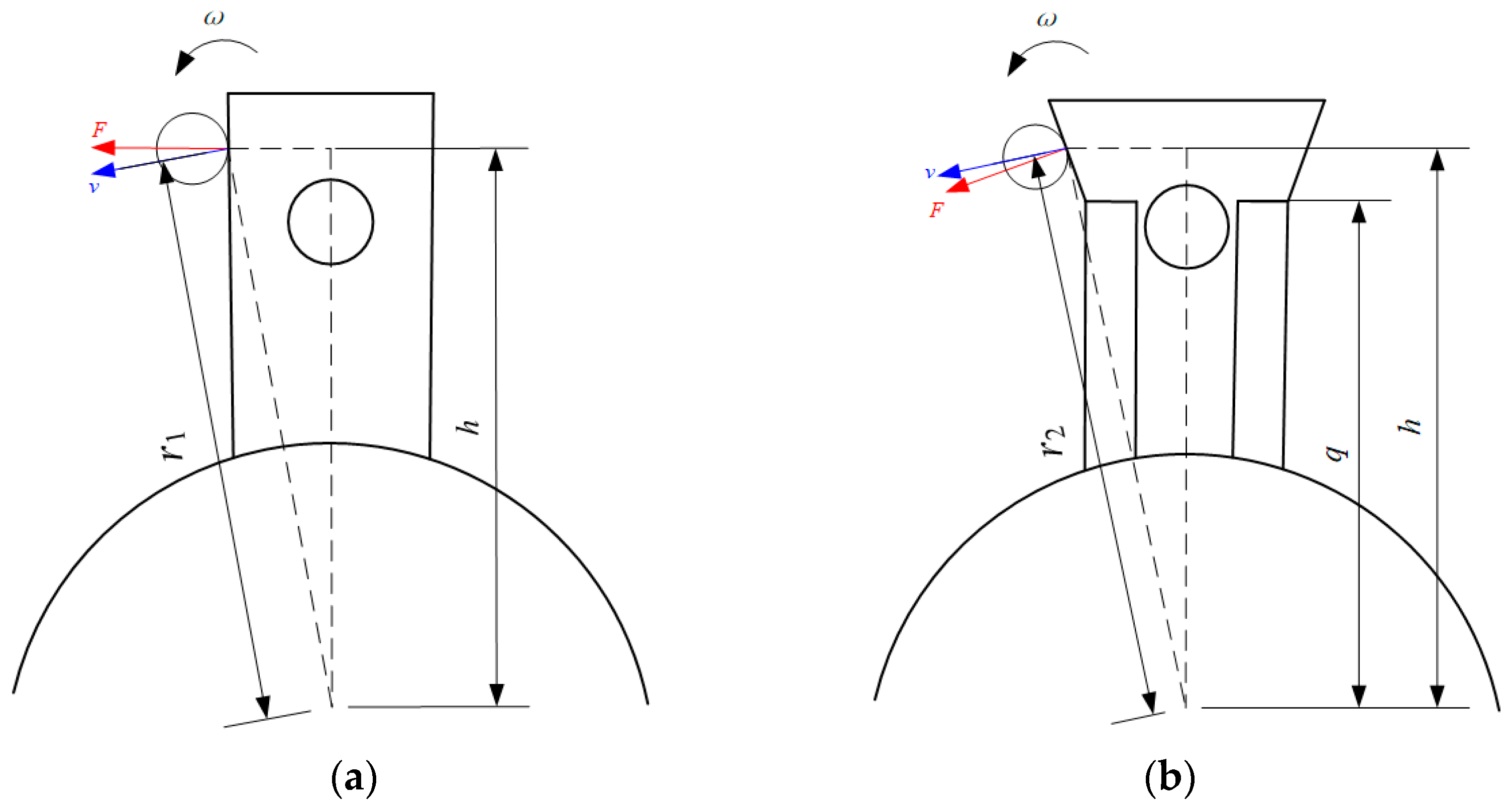
Figure 3.
Simulation environment.

Figure 4.
Jun-Cao stalks.

Figure 5.
Environment of bench test.

Figure 6.
Velocity distribution of Jun-Cao particles in the beginning of operation.
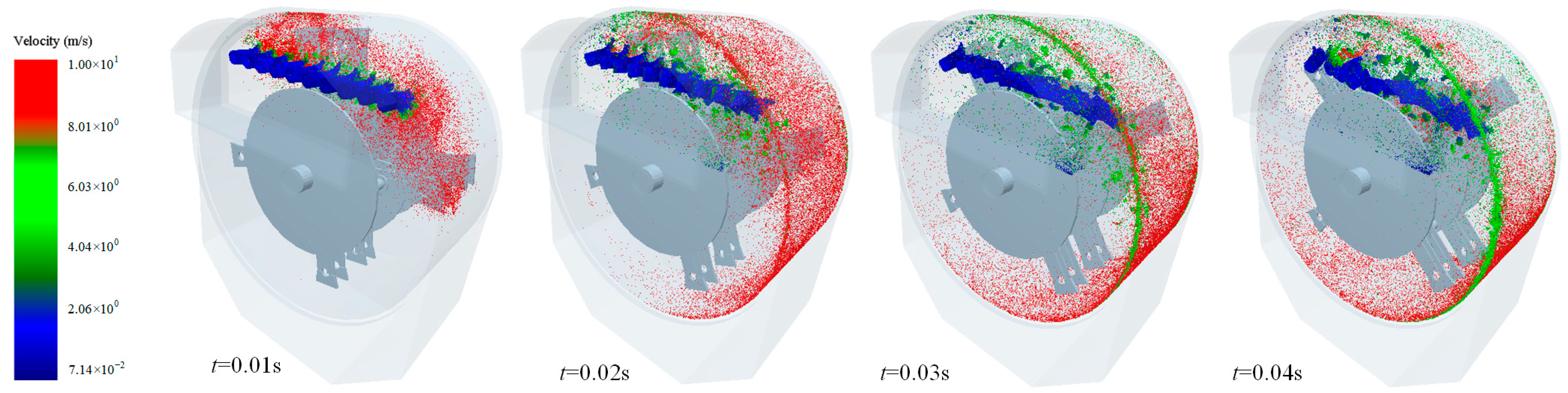
Figure 7.
Velocity of Jun-Cao particles after the operation became stable.
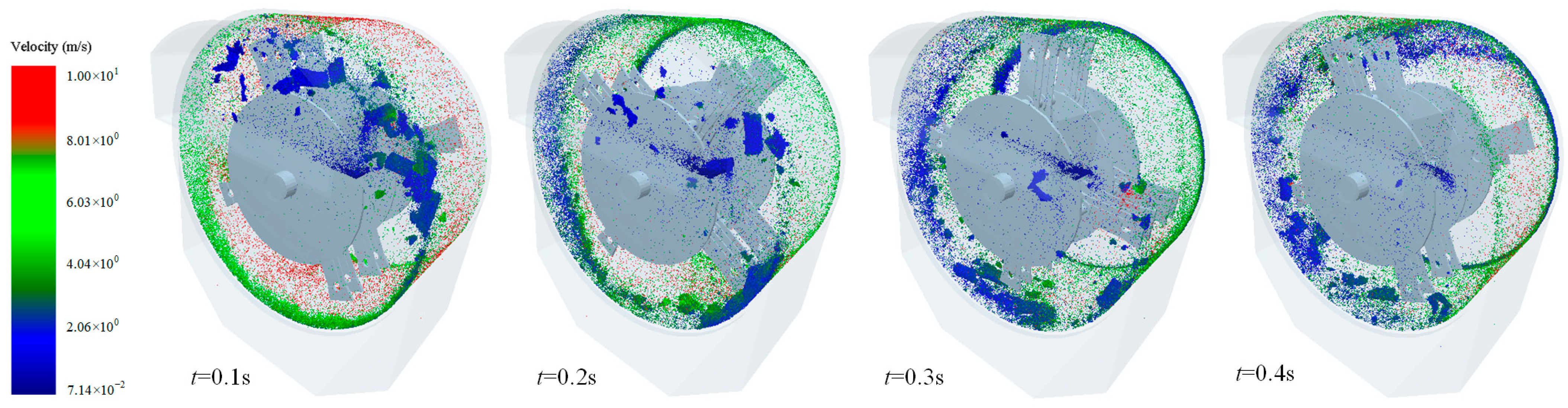
Figure 8.
Grinding of Jun-Cao stalks.
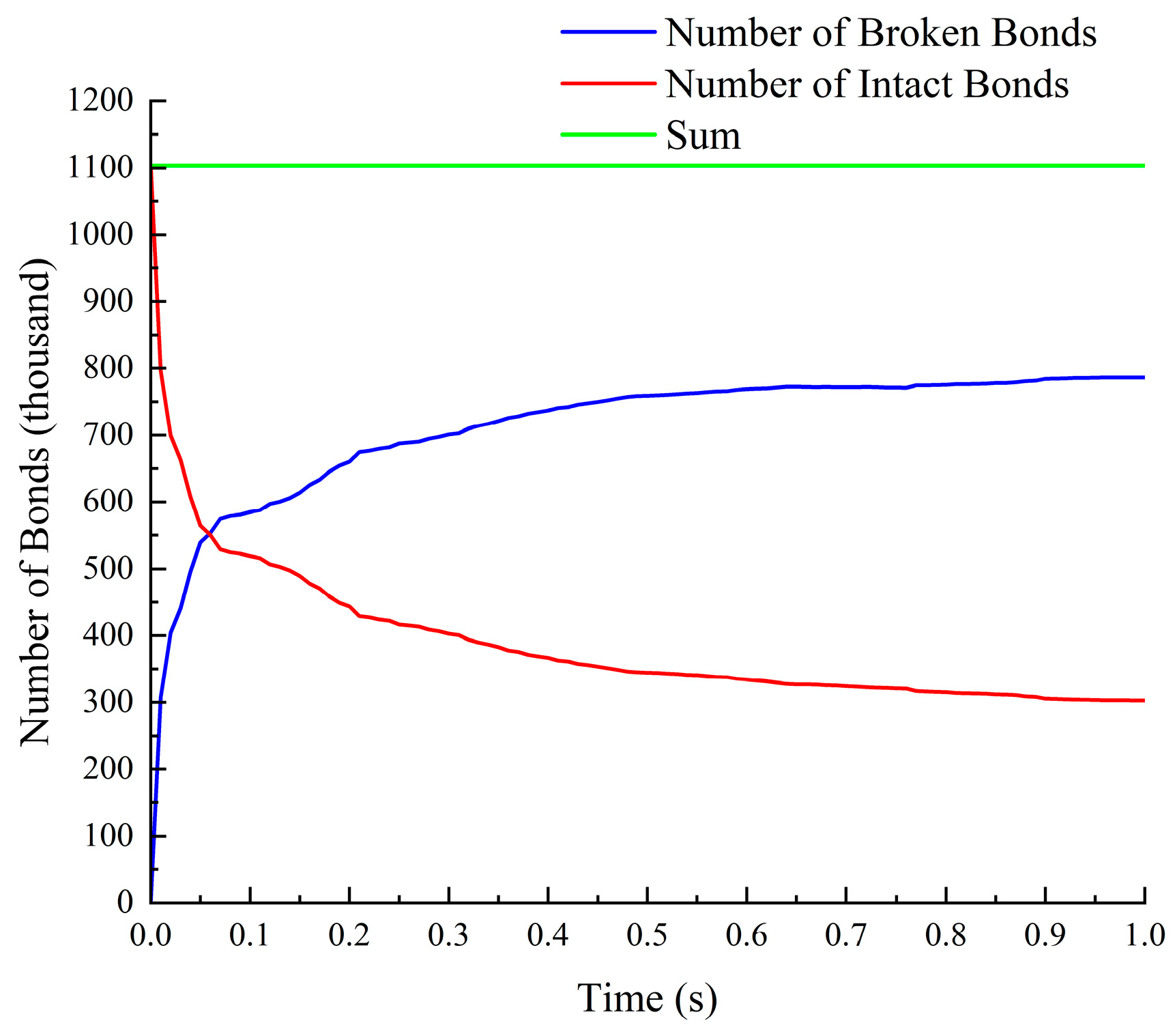
Figure 9.
Response curve for the number of broken bonds. (a) Interaction between A and B. (b) Interaction between A and C. (c) Interaction between B and C.
Figure 9.
Response curve for the number of broken bonds. (a) Interaction between A and B. (b) Interaction between A and C. (c) Interaction between B and C.

Figure 10.
Mean power response surface. (a) Interaction between A and B. (b) Interaction between A and C. (c) Interaction between B and C.
Figure 10.
Mean power response surface. (a) Interaction between A and B. (b) Interaction between A and C. (c) Interaction between B and C.

Figure 11.
Iteration process. (a) Power variation. (b) Changes in the number of broken bonds.
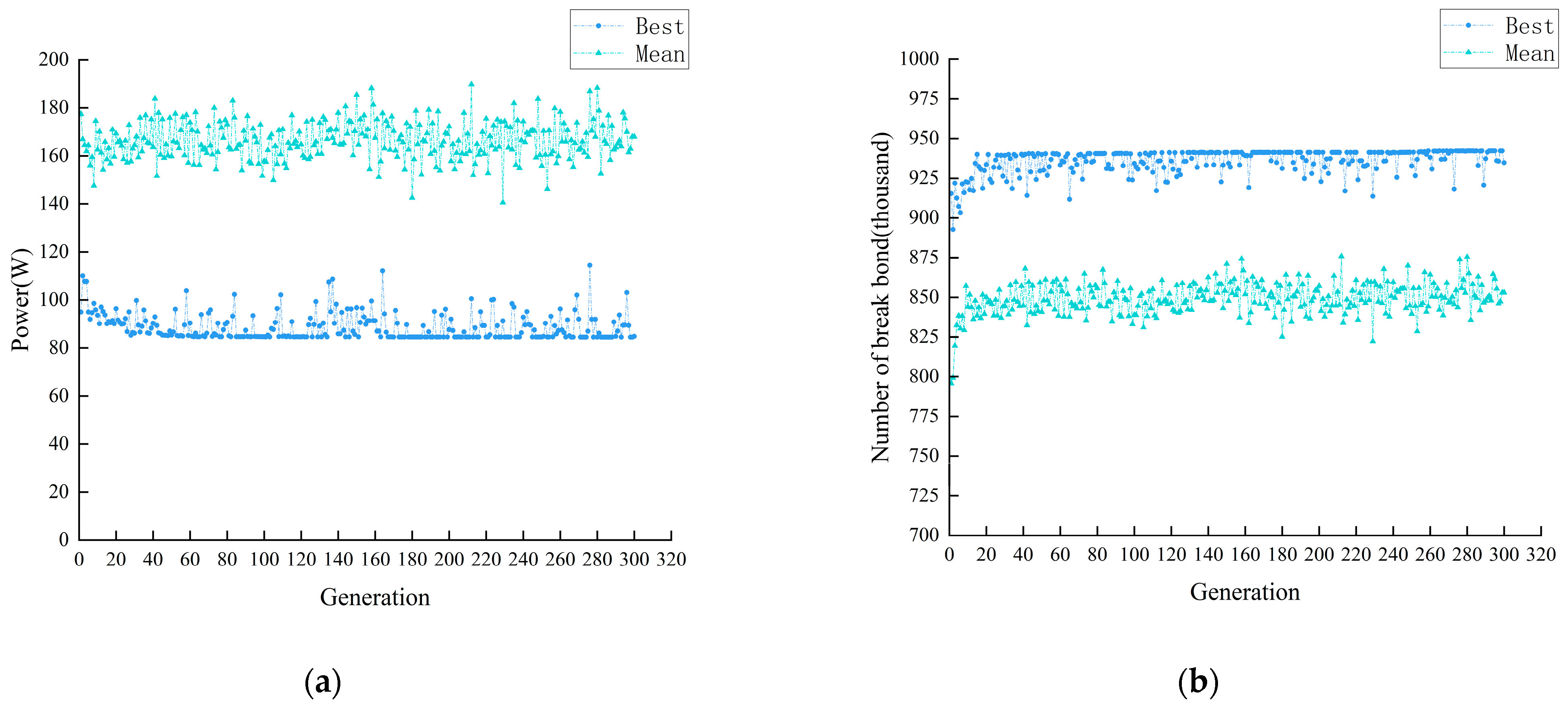
Figure 12.
Comparison test histogram.


Table 1.
Coefficients of the contact between particles.
| Particle–Blade | Particle–Particle | |
|---|---|---|
| Coefficient of Restitution | 0.2 | 0.2 |
| Coefficient of Static Friction | 0.4 | 0.7 |
| Coefficient of Rolling Friction | 0.01 | 0.01 |
Table 2.
Parameters of bonds.
| Normal Stiffness per Unit Area (N/mm2) | Shear Stiffness per Unit Area (N/mm2) | Critical Normal Stress (MPa) | Critical Shear Stress (MPa) | Bonded Disk Radius (mm) |
|---|---|---|---|---|
| 9.6 | 6.8 | 8.72 | 7.5 | 0.7 |
Table 3.
Factor level table in CCD test.
| Level | Factor | ||
|---|---|---|---|
| Cutting Edge Length A (mm) | Cutting Edge Thickness B (mm) | Hammer Thickness C (mm) | |
| 1.68179 | 51.8179 | 3.68179 | 8.36359 |
| 1 | 45 | 3 | 7 |
| 0 | 35 | 2 | 5 |
| −1 | 25 | 1 | 3 |
| −1.68179 | 18.1821 | 0.318207 | 1.63641 |
Table 4.
Simulation result.
| NO | Cutting Edge Length (mm) | Cutting Edge Thickness (mm) | Hammer Thickness (mm) | Bond Breakages Y | Power P |
|---|---|---|---|---|---|
| 1 | 35 | 2 | 1.636414 | 815,325 | 212.863 |
| 2 | 35 | 2 | 5 | 766,235 | 252.583 |
| 3 | 35 | 2 | 5 | 796,321 | 132.415 |
| 4 | 25 | 3 | 3 | 676,716 | 142.495 |
| 5 | 35 | 2 | 5 | 786,179 | 185.024 |
| 6 | 35 | 2 | 8.363586 | 742,066 | 212.831 |
| 7 | 35 | 2 | 5 | 776,444 | 91.236 |
| 8 | 35 | 0.318207 | 5 | 889,978 | 82.354 |
| 9 | 45 | 3 | 7 | 769,340 | 107.974 |
| 10 | 35 | 3.681793 | 5 | 710,325 | 134.311 |
| 11 | 45 | 1 | 3 | 956,745 | 281.102 |
| 12 | 25 | 3 | 7 | 621,773 | 110.278 |
| 13 | 35 | 2 | 5 | 783,024 | 207.455 |
| 14 | 45 | 3 | 3 | 839,703 | 134.956 |
| 15 | 18.18207 | 2 | 5 | 613,889 | 179.408 |
| 16 | 25 | 1 | 3 | 769,213 | 182.021 |
| 17 | 51.81793 | 2 | 5 | 882,481 | 181.112 |
| 18 | 25 | 1 | 7 | 733,801 | 165.231 |
| 19 | 45 | 1 | 7 | 917,241 | 172.365 |
| 20 | 35 | 2 | 5 | 796,151 | 162.354 |
Table 5.
Regression analysis on the number of broken bonds.
| Source | Sum of Squares | df | Mean Square | F-Value | p-Value | |
|---|---|---|---|---|---|---|
| Model | 1.489 × 10¹¹ | 9 | 1.654 × 10¹⁰ | 131.21 | <0.0001 | significant |
| A—Cutting edge length | 9.404 × 10¹⁰ | 1 | 9.404 × 10¹⁰ | 745.95 | <0.0001 | |
| B—Cutting edge thickness | 4.360 × 10¹⁰ | 1 | 4.360 × 10¹⁰ | 345.83 | <0.0001 | |
| C—Hammer thickness | 7.660 × 10⁹ | 1 | 7.660 × 10⁹ | 60.76 | <0.0001 | |
| AB | 4.563 × 10⁸ | 1 | 4.563 × 10⁸ | 3.62 | 0.0863 | |
| AC | 4.759 × 10⁷ | 1 | 4.759 × 10⁷ | 0.3775 | 0.5527 | |
| BC | 3.174 × 10⁸ | 1 | 3.174 × 10⁸ | 2.52 | 0.1437 | |
| A2 | 1.586 × 10⁹ | 1 | 1.586 × 10⁹ | 12.58 | 0.0053 | |
| B2 | 8.957 × 10⁸ | 1 | 8.957 × 10⁸ | 7.11 | 0.0237 | |
| C2 | 1.279 × 10⁶ | 1 | 1.279 × 10⁶ | 0.0101 | 0.9218 | |
| Residual | 1.261 × 10⁹ | 10 | 1.261 × 10⁸ | |||
| Lack of Fit | 5.828 × 10⁸ | 5 | 1.166 × 10⁸ | 0.8598 | 0.5638 | not significant |
| Pure Error | 6.778 × 10⁸ | 5 | 1.356 × 10⁸ | |||
| Cor Total | 1.501 × 10¹¹ | 19 |
Table 6.
Regression analysis on mean power.
| Source | Sum of Squares | df | Mean Square | F-Value | p-Value | |
|---|---|---|---|---|---|---|
| Model | 50,251.46 | 9 | 5583.50 | 145.46 | <0.0001 | significant |
| A—Cutting edge length | 935.29 | 1 | 935.29 | 24.37 | 0.0006 | |
| B—Cutting edge thickness | 36,094.21 | 1 | 36,094.21 | 940.30 | <0.0001 | |
| C—Hammer thickness | 61,93.76 | 1 | 6193.76 | 161.35 | <0.0001 | |
| AB | 549.94 | 1 | 549.94 | 14.33 | 0.0036 | |
| AC | 119.16 | 1 | 119.16 | 3.10 | 0.1086 | |
| BC | 142.21 | 1 | 142.21 | 3.70 | 0.0832 | |
| A2 | 4765.15 | 1 | 4765.15 | 124.14 | <0.0001 | |
| B2 | 962.57 | 1 | 962.57 | 25.08 | 0.0005 | |
| C2 | 3.38 | 1 | 3.38 | 0.0879 | 0.7729 | |
| Residual | 383.86 | 10 | 38.39 | |||
| Lack of Fit | 24.88 | 5 | 4.98 | 0.0693 | 0.9946 | not significant |
| Pure Error | 358.98 | 5 | 71.80 | |||
| Cor Total | 50,635.32 | 19 |
Table 7.
Optimal solution set.
| NO | Cutting Edge Length A (cm) | Cutting Edge Thickness B (cm) | Hammer Thickness C (cm) | Mean Power P (W) | Bond Breakages Y |
|---|---|---|---|---|---|
| 1 | 44.82853 | 1.00095 | 3.307438 | 249.2335 | 942,207 |
| 2 | 44.64202 | 2.749034 | 6.77861 | 99.40951 | 776,673 |
| 3 | 44.78693 | 2.563106 | 6.285873 | 115.5931 | 796,607 |
| 4 | 44.77821 | 2.326065 | 3.308412 | 167.8739 | 857,209 |
| 5 | 44.61134 | 2.292815 | 6.678316 | 125.7945 | 805,974 |
| 6 | 44.77056 | 1.016407 | 5.323537 | 227.4555 | 917,816 |
| 7 | 44.60674 | 1.360267 | 4.439888 | 212.391 | 901,019 |
| 8 | 44.80452 | 1.055466 | 3.553889 | 242.8482 | 935,216 |
| 9 | 44.82853 | 1.00095 | 3.307438 | 249.2335 | 942,207 |
| 10 | 44.71996 | 1.327035 | 4.93091 | 209.0372 | 898,135 |
| 11 | 44.72309 | 2.339939 | 6.167452 | 129.6454 | 811,675 |
| 12 | 44.46905 | 2.999992 | 6.999936 | 84.47981 | 757,836 |
| 13 | 44.61393 | 1.494478 | 5.781409 | 187.9295 | 874,194 |
| 14 | 44.71191 | 2.405573 | 3.703941 | 158.9335 | 846,445 |
| 15 | 44.69724 | 2.773154 | 6.386208 | 103.6859 | 782,334 |
| 16 | 44.75528 | 1.711658 | 5.346553 | 178.142 | 865,311 |
| 17 | 44.70631 | 2.073342 | 4.74662 | 163.4733 | 849,753 |
| 18 | 44.56903 | 2.929922 | 6.876811 | 89.28089 | 764,388 |
| 19 | 44.58156 | 1.687903 | 5.727792 | 175.56 | 860,661 |
| 20 | 44.79108 | 2.53502 | 4.598853 | 140.309 | 825,753 |
| 21 | 44.66016 | 1.862043 | 4.280812 | 181.79 | 869,405 |
| 22 | 44.71035 | 1.11735 | 4.054677 | 233.3952 | 924,197 |
Table 8.
Experimental result through the traditional rectangular hammer.
| NO | Operating Mass (kg) | Power Consumption (kW·h) | Output Per Kilowatt-Hour (kg·(kW·h)−1) |
|---|---|---|---|
| 1 | 19.94 | 1.1 | 18.13 |
| 2 | 17.11 | 0.9 | 19.01 |
| 3 | 18.67 | 1 | 18.67 |
| 4 | 18.72 | 1 | 18.72 |
| 5 | 19.29 | 1.1 | 17.54 |
| Mean | 18.78 | 1.02 | 18.41 |
Table 9.
Experimental result through our new hammer.
| NO | Operating Mass (kg) | Power Consumption (kW·h) | Output Per Kilowatt-Hour (kg·(kW·h)−1) |
|---|---|---|---|
| 1 | 21.41 | 1 | 21.41 |
| 2 | 22.91 | 1.1 | 20.83 |
| 3 | 18.50 | 0.9 | 20.56 |
| 4 | 21.71 | 1 | 21.71 |
| 5 | 18.01 | 0.9 | 20.01 |
| Mean | 20.49 | 0.98 | 20.90 |
Disclaimer/Publisher’s Note: The statements, opinions and data contained in all publications are solely those of the individual author(s) and contributor(s) and not of MDPI and/or the editor(s). MDPI and/or the editor(s) disclaim responsibility for any injury to people or property resulting from any ideas, methods, instructions or products referred to in the content. |
© 2024 by the authors. Licensee MDPI, Basel, Switzerland. This article is an open access article distributed under the terms and conditions of the Creative Commons Attribution (CC BY) license (https://creativecommons.org/licenses/by/4.0/).
Share and Cite
MDPI and ACS Style
Zheng, S.; Chen, C.; Guo, Y. Analysis and Structural Optimization Test on the Collision Mechanical Model of Blade Jun-Cao Grinding Hammer. Agriculture 2024, 14, 492. https://doi.org/10.3390/agriculture14030492
AMA Style
Zheng S, Chen C, Guo Y. Analysis and Structural Optimization Test on the Collision Mechanical Model of Blade Jun-Cao Grinding Hammer. Agriculture. 2024; 14(3):492. https://doi.org/10.3390/agriculture14030492
Chicago/Turabian StyleZheng, Shuhe, Chongcheng Chen, and Yuming Guo. 2024. "Analysis and Structural Optimization Test on the Collision Mechanical Model of Blade Jun-Cao Grinding Hammer" Agriculture 14, no. 3: 492. https://doi.org/10.3390/agriculture14030492
Note that from the first issue of 2016, this journal uses article numbers instead of page numbers. See further details here.