Automated Grading of Angelica sinensis Using Computer Vision and Machine Learning Techniques

Abstract

Angelica sinensis (Oliv.) Diels, a member of the Umbelliferae family, is commonly known as Danggui (Angelica sinensis, AS). AS has the functions of blood tonic, menstrual pain relief, and laxatives. Accurate classification of AS grades is crucial for efficient market management and consumer health. The commonly used method to classify AS grades depends on the evaluator’s observation and experience. However, this method has issues such as unquantifiable parameters and inconsistent identification results among different evaluators, resulting in a relatively chaotic classification of AS in the market. To address these issues, this study introduced a computer vision-based approach to intelligently grade AS. Images of AS at five grades were acquired, denoised, and segmented, followed by extraction of shape, color, and texture features. Thirteen feature parameters were selected based on difference and correlation analysis, including tail area, whole body area, head diameter, G average, B average, R variances, G variances, B variances, R skewness, G skewness, B skewness, S average, and V average, which exhibited significant differences and correlated with grades. These parameters were then used to train and test both the traditional back propagation neural network (BPNN) and the BPNN model improved with a growing optimizer (GOBPNN). Results showed that the GOBPNN model achieved significantly higher average testing precision, recall, F-score, and accuracy (97.1%, 95.9%, 96.5%, and 95.0%, respectively) compared to the BPNN model. The method combining machine vision technology with GOBPNN enabled efficient, objective, rapid, non-destructive, and cost effective AS grading.

1. Introduction

Angelica sinensis (Oliv.) Diels is a plant belonging to the Umbelliferae family. Its root is a widely used medicine–food Chinese medicinal herb known as Danggui (Angelica sinensis, AS) [1,2]. AS is rich in polysaccharides, essential oils, flavonoids, and organic acids [3,4]. AS is often used to treat blood deficiency, menstrual disorders, and constipation due to its properties as a blood tonic, menstrual pain reliever, and laxative [5,6,7].

The grade of Chinese medicinal herbs plays an important role in evaluating its quality as well as determining its market price [8]. The “Specifications and Grading Standards for Chinese Medicinal Materials” provides grading criteria for AS. The standard indicates that, under the conditions of no mildew, no insect damage, no oil exudation, impurities less than 3%, and meeting specific appearance characteristics (the upper main root is cylindrical, or has several distinct protruding rhizome scars, with multiple lateral roots in the lower part, and the root tip diameter is 0.3~1 cm. The surface is brownish-yellow or yellow-brown, with longitudinal wrinkles and pore-like protrusions, which may be inconspicuous or absent, and the texture is soft and flexible). The quantity of AS per kilogram and the weight of each AS are used as indicators for grading [9]. The commonly used method for classifying AS commodity grades is a traditional method based on the observation and experience of the evaluator. This method has issues such as high subjectivity, unquantifiable parameters, inconsistent identification results among different evaluators, and a long learning curve to master this skill, resulting in a relatively chaotic grading of AS in the market. The disordered grades fail to meet the demands of consumers for both the quality and safety of Chinese medicinal herbs [10]. Additionally, the process of determining the grade of AS based on the observer’s observation and experience is time-consuming, labor-intensive, and subjective.

To address the issue of high subjectivity in this method, many scientists have conducted research on the classification of AS grades based on chemical composition. Xin et al. used a dual-wavelength thin film scanning method to determine the ferulic acid content of different grades of AS [11]. Their findings revealed notable variations in the ferulic acid content among different AS grades, with higher grades exhibiting higher levels of ferulic acid. Zhao found that the commodity grade of AS could be determined on the basis of its chemical composition [12]. His results showed that chlorogenic acid was significantly negatively correlated with the commodity grade of AS, while ferulic acid and Z-ligustilide were significantly positively correlated with the commodity grade of AS. The aforementioned studies suggested that chemical composition appeared to be a viable indicator for grading by a quantitative method. However, Ruan et al. found that polysaccharide and ferulic acid had a very weak negative correlation with AS commodity grade, indicating that the content of these compounds could not be considered good indicators of the commodity grade of AS [13]. In conclusion, the content of a specific chemical component may not necessarily be a reliable indicator for grading AS products. Moreover, the cost of testing the chemical composition is relatively high, and it takes a long time to obtain results, which makes it difficult to widely apply this method for classifying the grades of AS. For this reason, it is necessary to develop a simpler, faster, and more effective method.

Machine vision technology enables an objective evaluation of Chinese medicinal material quality, significantly reducing the time, costs, and labor required for analyses [14]. In recent years, machine vision technology has been widely applied in the fields of medicine and food [15,16,17,18,19]. Kim et al. used image processing technology and an artificial neural network to divide ginseng into three grades based on its color and shape features. The classification error was about 26% [20]. Cui et al. developed a vision system that took into account the color features of Cornus officinalis. They used discriminant analysis, least squares support vector machine, partial least squares discriminant analysis, and principal component discriminant analysis to evaluate the grade of Cornus officinalis, and the accuracy was 86.21%, 89.66%, 81.03%, and 91.38%, respectively [21]. Wang et al. used a back-propagation neural network (BPNN) to classify rhubarb grades based on color features extracted from images and achieved an overall accuracy of 92.3% [22]. Zhu et al. used an improved IRIV-GWO-SVM (IRIV: iterative retaining information variables; GWO: gray wolf optimizer; SVM: support vector machine) model to classify the taproot of Notoginseng based on the color, texture, and shape features from computer vision, and the accuracy reached 98.70% [23]. These results indicated that machine vision technologies combined with machine learning had the potential to classify the grades of some Chinese medicinal materials. However, there are no studies using these techniques to classify the grades of AS.

Considering the limitation of sample data size, this study chose a three-layer BPNN model with good generalization ability in small sample data for the identification of AS grades [24,25]. The BPNN model was proposed by a scientific team led by Rumelhart and McClelland [26]. It has been largely used for classification due to its high non-linear mapping, self-learning, and adaptability, and has achieved satisfactory results [27]. Unfortunately, the standard version of BPNN has its limitations, such as a tendency to fall into local minima and slow convergence [28]. To overcome these problems, this study used a growth optimizer (GO) developed in 2023 to optimize the weights (w) and deviations (b) of BPNN to obtain better results in the classification of AS grades [29]. The primary design inspiration for GO originates from the learning and reflective mechanisms of humans during the course of social development [29]. Through the mathematical modeling of learning and reflection behaviors, GO is categorized into two phases: The learning stage and the reflection stage. The learning stage of GO dynamically balances four types of directional information by incorporating fitness values and Euclidean distance. This adaptive balancing is crucial in mitigating the impact of incorrect directional information, significantly diminishing the likelihood of the algorithm succumbing to local optima. The reflection stage of GO uses distinct computation methods for each dimension of the individual, thereby augmenting the overall convergence performance of GO. These advantages of GO are helpful in overcoming the shortcomings of BPNN. In this study, the BPNN model optimized by using the GO algorithm was named GOBPNN.

In order to address the limitations of the method of classifying AS grades based on the evaluator’s observation and experience, such as high subjectivity, unquantifiable parameters, inconsistent identification results among different evaluators, and a long learning curve to master this skill, this study combined computer vision with the GOBPNN model to achieve intelligent recognition of AS grades through image analysis. The findings of this study will facilitate efficient, objective, fast, non-destructive, and low-cost classification of the grades of AS, which could help consumers and market regulatory authorities to quickly and accurately identify the grade of AS.

2. Materials and Methods

The image recognition system was divided into four stages: (a) image acquisition; (b) image pre-processing; (c) image feature extraction; and (d) classification decision.

2.1. Samples Preparation

Standard samples of AS were purchased from Minxian County, Gansu Province, in 2021. They were divided into five commodity grades according to industry association standards [9] and the experience of Chinese herbal medicine experts, who has gained recognition from relevant companies and consumers. The original AS images representing five grades are shown in Figure 1. These standard samples (Figure 1) exhibit distinctive external characteristics, primarily comprising color, shape, and texture features. The number of AS for each grade and the weight of individual AS samples for each grade are shown in

Table 1. The number of AS for each grade and the weight of individual AS for each grade.

Grade	Number of AS	Weight of Each AS (g)
Grade one	49	>60
Grade two	140	25~60
Grade three	110	15~25
Grade four	44	10~15
Grade five	54	<10
Total	397

.

2.2. Image Acquisition

In order to obtain high-quality images, an image acquisition system was designed, and its structure diagram is shown in Figure 2. The image acquisition system mainly included a charge-coupled device (CCD) camera (Basler AG, Arnsberg, Germany, aca250014-gc), FA lens (Computar, Tokyo, Japan, M1214-MP2), and LED light (Shanghai Jia Ken Photoelectric Technology Co., Ltd., Shanghai, China, JKVR-170W). The Basler camera used for the current work was 2.2-megapixel RGB camera with a resolution of 2590 × 1942, a CMOS sensor, full resolution at a maximum frame rate of 14 fps, and an effective operating temperature range of 0 to 50 °C. Non-reflective black fabric was used to completely wrap the outside of the frame of the whole collecting system, and another side was left open to place the AS samples. OpenCV (version 3.0) was used to capture and save sample images.

During the image acquisition process, in order to ensure that images of AS of different sizes could be fully captured and to ensure the clarity of the photos, the samples were placed at a distance of 40 cm from the camera. In order to ensure a uniform background, white paper was placed on the loading platform. Then, the samples were arranged horizontally on the white background. To ensure accurate measurement of the length and area of AS, a ruler with a scale was placed to the right of AS at a specified distance. To obtain the appropriate lighting conditions, the brightness of the LED lamp was set at 1210 lm. Both the images of the front and back sides of each AS sample were acquired using the image acquisition system. A total of 794 images were collected. The image size was 2590 pixels by 1942 pixels. The file format for the images was tiff. To ensure consistency in the number of images across each grade, 80 images were randomly selected for each grade. Among these, 70% of the data is allocated for the training set, 15% for the validation set, and the remaining 15% for the test set. The training set was utilized to “teach” the model to recognize data, the validation set was utilized to “tune” the model parameters during training and prevent overfitting, and the test set was utilized to “evaluate” the generalization ability and final performance of the model after the model development was complete [30].

2.3. Pre-Processing and Segmentation

Image pre-processing is an essential step in pattern recognition systems. The process involves a series of steps, such as reducing noise and image segmentation. In this work, a relatively effective mean filter was used for image denoising. Image segmentation is an important element of the system, as it allows for advanced image analysis and understanding. In this work, the denoised image underwent binarization and an opening operation using the OTSU method [31]. Next, the original RGB image was multiplied by the processed binarization matrix to extract the background area. Finally, the background area was subtracted from the original RGB image, and an accurate AS image segmentation was obtained, which was used in further analysis.

2.4. Feature Extraction

After performing the segmentation step, AS images without the white background were obtained. From the segmented images of AS, shape features, color features, and texture features could be extracted.

2.4.1. Extraction of Shape Features

The whole body of AS consists of the head and the tail, as shown in Figure 3. The various parts of AS exhibit distinct differences in their efficacy and medicinal properties, as reported by Chen et al. [32]. Therefore, when extracting the shape features of AS, the shape features of the head, the tail, and the whole body were all extracted.

To extract the shape features of the head, tail, and whole body, the widely adopted DeepLabv3+ semantic segmentation [33], which has high segmentation accuracy and precision, was first used to distinguish the head and tail of AS, and then the area, length, and diameter of the head, tail, and whole body were calculated. Additionally, the number of tail roots and average diameter of tail roots were also calculated. The operating system and environment were Microsoft Windows 10 and Python3.6 compilation, respectively, and the deep learning frameworks CUDAToolkit9.0 and Paddle-GPU2.2.0 were also installed.

A total of 794 images were collected to construct the semantic segmentation dataset. Using the image annotation tool Labelme, manual annotations were performed on the heads, tails, and individual tail roots of each image. For each AS image, two types of annotation images were created: The first annotation image, as shown in Figure 4B, annotated the heads and tails, with the remaining parts as background, used to train the model for segmentation of heads and tails. The second annotation image, illustrated in Figure 4C, annotated recognizable and relatively complete roots in Angelica images and was used to train the model for segmentation of each root. In the first annotation image, the AS tail was annotated as a whole, while in the second annotation image, each root was individually marked instead of treating the AS tail as a whole.

The labeled data were randomly divided into training set, validation set, and test set at a ratio of 6:2:2, where the training set contained 476 images and the validation set and test set contained 159 images, respectively. In order to ensure that the number of input images of the deep learning network met the requirements, data enhancement was performed on the training set images, including random distortion, brightness adjustment, saturation adjustment, and contrast adjustment.

The training process was designed using the PaddlePaddle framework, the optimizer uses SGD, and the loss function was the cross-entropy loss function. After repeated tests, the parameters were set as follows: Learning rate = 0.001, momentum = 0.1, weight decay = 0.00001, batch size = 10, and the number of training iterations was 400. The training results showed that the intersection-over-union (IoU) and recall rate of both the tail and single-branched tail root exceeded 80%, indicating effective recognition. AS images were randomly selected from the test set for specific semantic segmentation effect verification, and the results are shown in Figure 5.

From the recognition effect in Figure 5, it was evident that the trained model performs well in recognizing the head and tail (comparing B with C in Figure 5) and the single tail root (comparing D with E in Figure 5). Therefore, this trained model can be applied to segment the heads, tails, and single-tail roots of other AS images.

The extraction steps for the diameter, length, and area of the head, tail, and whole body of AS are shown in Figure 6. Taking the head of AS as an example, the quantification process of its length, diameter, and area was presented as follows: (1) The semantic segmentation results of the head and tail (Figure 6B) were first grayscaled (Figure 6C); (2) since the grayscale values of the head, tail, and background pixels are different, the gray level of the head pixels was set to 255 and the gray level of all other pixels was set to zero (Figure 6D); (3) a binary image of the AS head was obtained (Figure 6E), the number of pixels in the area occupied by the head was obtained, and the head area could be calculated by multiplying the area of each pixel (6.0279 × 10⁻⁵ cm²) by the pixel count; (4) based on the binary image of the AS head, a minimum bounding rectangle of the AS head was created (Figure 6F); (5) the diameter of the head was equal to the number of horizontal pixels of the bounding rectangle multiplied by the length of each pixel (0.00776397 cm), and the length of the head was equal to the number of pixels in the vertical direction of the bounding rectangle multiplied by the length of each pixel.

The quantification methods for the diameter, length, and area of the tail of AS were the same as the quantification methods used for the head, as shown in Figure 6G–I. The quantification methods for the diameter, length, and area of the whole body of AS were the same as the quantification methods used for the head, as shown in Figure 6J–L.

The steps of extraction of the number and average diameter of tail roots in AS are shown in Figure 7. First, the semantic recognition of the tail roots of AS was carried out. The semantic segmentation result (Figure 7B) was converted to a gray-scale image (Figure 7C) and then a binary image (Figure 7D). All the identified tail roots were treated as a single entity, and the minimum bounding rectangle was created for this entity (Figure 7E). A horizontal line was drawn at the upper quarter of this rectangle in the vertical direction (Figure 7F). A logical AND operation was performed between the horizontal line and the tail roots of AS to obtain overlapping line segments (Figure 7G). The number of overlapping line segments represented the number of tail roots, and the average number of pixels in the horizontal direction of these segments multiplied by the actual length of each pixel (0.00776397 cm) was the average diameter of the tail roots.

A total of 19 shape feature parameters were extracted, including head length, tail length, whole body length, head diameter, tail diameter, whole body diameter, head area, tail area, whole body area, head diameter-to-length ratio (i.e., the ratio of head diameter to head length), tail diameter to length ratio, whole body diameter to length ratio, head to tail length ratio (i.e., the ratio of head length to tail length), head to whole body length ratio, head to tail diameter ratio (i.e., the ratio of head diameter to tail diameter), head to tail area ratio (i.e., the ratio of head area to tail area), head to whole body area ratio, mean diameter of tail roots and number of tail roots.

2.4.2. Extraction of Color Features

In the “Chinese Medicinal Materials Commercial Specifications and Grade Standards” [9], the surface color of first-grade AS ranges from brownish-yellow to yellow-brown. The color features should be quantified.

Color features are pixel-level features of images with advantages such as rotation, scale, and translation invariance. This study selected the common digital image color spaces RGB (red, green, blue) and HSV (hue, saturation, value) as the spatial descriptors for color features. The color moment fully represented the color distribution features of the image, and the color distribution information was mainly concentrated in the first-order moment (M_i1), second-order moment (M_i2), and third-order moment (M_i3). The formulas for calculating the first three color moments are as follows:

$$M_{i1}=\frac{1}{N}\sum _{j=1}^N{P_i}_j$$

(1)

$$M_{i2}=\left(\frac{1}{N}\right.{\left.\sum _{j=1}^N\left({P_i}_j\right.-{\left.{M_i}_1\right)}^2\right)}^{\raisebox{1ex}{$1$}\!\left/ \!\raisebox{-1ex}{$2$}\right.}$$

(2)

$$M_{i3}=\left(\frac{1}{N}\right.{\left.\sum _{j=1}^N\left({P_i}_j\right.-{\left.{M_i}_1\right)}^3\right)}^{\frac{1}{3}}$$

(3)

where i1 represented R and H component; i2 represented G and S component; i3 represented B and V component; P_ij represented the color value of the j-th pixel on the i-th color channel; and N represented the number of pixels in the image.

A total of 18 color feature parameters were extracted, including R average, G average, B average, R variance, G variance, B variance, R skewness, G skewness, B skewness, H average, S average, V average, H variance, S variance, V variance, H skewness, S skewness, and V skewness.

2.4.3. Extraction of Texture Features

In the “Chinese Medicinal Materials Commercial Specifications and Grade Standards” [9], first-grade AS displays the following characteristics: The head exhibits clear root and rhizome marks; the body presents longitudinal wrinkles, with inconspicuous or absent pore-like elevations; and it possesses a soft and flexible texture. These texture features should be quantified as well.

The texture feature is a measure of roughness, contrast, directivity, linearity, and regularity [34]. The gray-level co-occurrence matrix (GLCM) is used to extract texture features [35]. The GLCM algorithm is easy to implement and has been proven to give very good results in a wide range of applications. GLCM has the following advantages: (1) It can capture spatial relationships between pixels, extracting texture information; (2) it is sensitive to grayscale variations, distinguishing subtle differences in different textures; (3) the algorithm is relatively simple and easy to implement; (4) it performs well in many application domains. Second-order statistics provide more in-depth information about the spatial distribution of pixel grayscale values, helping analyze the texture structure of images. For example, energy (ASM) reflects the degree of contrast of grayscale levels in the image, entropy (ENT) characterizes the complexity of image texture, correlation (COR) measures the degree of correlation of grayscale levels in the image, while contrast (CON) indicates the degree of difference in grayscale levels in the image.

$$\mathit{ASM}={\sum }_i{\sum }_j{P(i,j)}^2$$

(4)

$$ENT=\sum _i\sum _{{\displaystyle j}}P\left(i,j\right){\displaystyle logP(i,j)}$$

(5)

$$\begin{gathered} COR=[\sum _i\sum _j\left(\left(ij\right)P\left(i,j\right)\right)-{\mu }_x{\mu }_y]/{\sigma }_x{\sigma }_y \\ {\mu }_1={\displaystyle \sum _{i=0}^{L-1}i}{\displaystyle \sum _{j=0}^{L-1}{\widehat{P}}_d}(i,j), {\mu }_2={\displaystyle \sum _{i=0}^{L-1}j}{\displaystyle \sum _{j=0}^{L-1}{\widehat{P}}_d}(i,j), \\ {\sigma }_1^2={\displaystyle \sum _{i=0}^{L-1}{\left(i-{\mu }_1\right)}^2}{\displaystyle \sum _{j=0}^{L-1}{\widehat{P}}_d}(i,j), {\sigma }_2^2={\displaystyle \sum _{i=0}^{L-1}{\left(i-{\mu }_1\right)}^2}{\displaystyle \sum _{j=0}^{L-1}{\widehat{P}}_d}(i,j) \end{gathered}$$

(6)

$$CON=[\sum _i\sum _j\left(\left(ij\right)P\left(i,j\right)\right)-{\mu }_x{\mu }_y]/{\sigma }_x{\sigma }_y$$

(7)

where i, j represented the grayscale of the pixel; L represented the gray level of the image; d represented the spatial position relationship between two pixels; and P_d(i, j) represented frequency of occurrence of two pixels with spatial position relation d and grayscale of i and j, respectively.

The texture analysis comprised eight distinct parameters, namely the average and standard deviation of ASM, ENT, COR, and CON, which were computed across four different directions, namely 0, 30, 60, and 90 degrees. A total of 8 texture feature parameters were extracted, including ASM average, ENT average, COR average, CON average, ASM standard deviation, ENT standard deviation, COR standard deviation, and CON standard deviation. By statistically analyzing these second-order statistics, a more precise understanding and description of the texture features in AS images can be achieved, establishing a stronger foundation for subsequent image analysis and processing.

2.5. Classification Model for AS Grades

2.5.1. The BPNN Model

The BPNN was a multi-layer perceptron trained with incremental learning rules, consisting of an input layer, one or more hidden layers, with each hidden layer containing several hidden nodes, and an output layer. The sigmoidal function was used as the activation function between the hidden and output layers. The gradient descent method was used to minimize the loss function, which was designed to measure the disparity between the model’s predicted results and the actual labels.

2.5.2. The GO Algorithm

The primary design inspiration for GO originates from the learning and reflective mechanisms of humans during the course of social development [29]. Learning is the process by which individuals assimilate knowledge from the external milieu and undergo personal development. Reflection entails scrutinizing individual limitations, adjusting learning methodologies, and fostering personal advancement. Through the mathematical modeling of learning and reflection behaviors, GO is categorized into two phases: the learning stage and the reflection stage.

During the learning stage, four hierarchical individuals were defined: Leader (${\overrightarrow{X}}_{best}$), elite (${\overrightarrow{X}}_{better}$), bottom layer (${\overrightarrow{X}}_{worst}$), and random individuals (${\overrightarrow{X}}_{L1}$) and (${\overrightarrow{X}}_{L2}$). Gaps between them were categorized as the leader-elite gap ($\overrightarrow{Gap1}$), leader-bottom layer gap ($\overrightarrow{Gap2}$), elite-bottom layer gap ($\overrightarrow{Gap3}$), and random individuals’ gap ($\overrightarrow{Gap4}$). Normalized gaps LF_k (k = 1, 2, 3, 4) and fitness ratios (SF_i (i = 1, 2, 3, 4)) for each individual were defined. The acquired knowledge was as $\overrightarrow{{KA}_k}$. Individuals assimilate knowledge gaps, completing a comprehensive process of knowledge accumulation. The learning process was expressed as ${{\overrightarrow{X}}_i}^{It+1}$, where it was the current iteration count, and learning quality changes are determined by P₂ and Equation (14).

$$\overrightarrow{Gap1}={\overrightarrow{X}}_{best}-{\overrightarrow{X}}_{better}$$

(8)

$$\overrightarrow{Gap2}={\overrightarrow{X}}_{best}-{\overrightarrow{X}}_{worst}$$

(9)

$$\overrightarrow{Gap3}={\overrightarrow{X}}_{better}-{\overrightarrow{X}}_{worst}$$

(10)

$$\overrightarrow{Gap4}={\overrightarrow{X}}_{L1}-{\overrightarrow{X}}_{L2}$$

(11)

$$\overrightarrow{{KA}_k}={SF}_i\times {LF}_k\times \overrightarrow{{Gap}_k},k=\mathrm{1,2},\mathrm{3,4}$$

(12)

$${{\overrightarrow{X}}_i}^{It+1}={{\overrightarrow{X}}_i}^{It}+\overrightarrow{{KA}_1}+\overrightarrow{{KA}_2}+\overrightarrow{{KA}_3}+\overrightarrow{{KA}_4}$$

(13)

$${\underset{x_i}{\to }}^{It+1}=\left\{\begin{array}{c}{\underset{x_i}{\to }}^{It+1} if f\left({\underset{x_i}{\to }}^{It+1}\right)<f\left({\underset{x_i}{\to }}^{It}\right)\\ \left\{\begin{array}{c}{\underset{x_i}{\to }}^{It+1} if r_1<P_2\\ {\underset{x_i}{\to }}^{It} else\end{array}\right. else\end{array}\right.$$

(14)

During the reflection stage, individuals were allowed to examine and remedy deficiencies. Positive aspects were retained, and when certain aspects were irremediable, past knowledge was discarded for a systematic relearning process. The reflection process of GO was mathematically modeled by Equations (15) and (16).

$${x_{i,j}}^{It+1}=\left\{\begin{array}{c}\left\{\begin{array}{c}lb+r_4\times \left(ub-lb\right) if r_3<AF\\ {x_{i,j}}^{It}+r_5\times (R_j-{x_{i,j}}^{It}) else\end{array}\right. if r_2<P_3\\ {x_{i,j}}^{It} else\end{array}\right.$$

(15)

$$AF=0.01+0.99\times \left(1-\frac{FEs}{MaxFEs}\right)$$

(16)

where ub and lb represented the upper and lower bounds of the search space, r₂, r₃, r₄, r₅ were random numbers uniformly distributed in the range [0, 1]. The parameter P₃ governed the probability of reflection and was typically set to 0.3. The decay factor AF was determined by the current evaluation count (FEs) and the maximum evaluation count (MaxFEs)). Over the course of algorithm iterations, the value of AF gradually converged to 0.01. This convergence signified that as individuals made progress, frequent reinitializations were used to prevent unnecessary time consumption. In the reflection phase, the j-th aspect of the i-th individual was influenced by certain superior individuals ($\overrightarrow{R}$). Here, $\overrightarrow{R}$ denoted individuals at a higher level, serving as guides for reflective learning in the context of the current individual i.

2.5.3. The GOBPNN Model

The proposed GOBPNN model utilized the GO algorithm to explore the parameter space of BPNN for seeking a broad global optimum, concurrently using the gradient descent algorithm to finely tune local regions, in order to optimize the parameter weights (w) and thresholds (b) of the BPNN, thereby accelerating model convergence and enhancing solution accuracy. The detailed procedure for implementing the GOBPNN model in AS grade classification is depicted in Figure 8.

And the steps of GOBPNN implementation can be summarized as follows:

(1)

Collected the AS images, and extracted features of AS images. Then selected features that were used for model training. Defined the architecture of the BPNN and network training parameters were configured, such as the maximum number of training epochs (epochs), learning rate (lr), target error (goal), display frequency (show), momentum factor (mc), minimum performance gradient (min_grad), and maximum number of failures (max_fail).

(2)

Initialized parameters, including population size (N), population dimension (D), iteration count (FEs), maximum iteration count (MaxFEs), upper bound of the search space (ub), and lower bound of the search space (lb).

(3)

Initialized the population (X) based on N, D, ub, and lb. The population represented a set of individuals, where an individual’s elements denoted crucial parameters (e.g., weights and biases). An individual was a row vector with D columns, forming an N row by D column matrix. The error between the output value and the target value of the neural network was used to calculate the fitness. The individual with the minimum fitness was defined as the optimal individual, gbestX.

(4)

Commenced the iterative process. Calculated the fitness of each individual in the population, sorted the fitness to find the current best individual (Best_X) and worst individual (Worst_X), continuously updated the best individual (Best_X) during iteration, and updated gbestX after each evaluation.

(5)

Learning phase: For the i-th individual, selected Better_X and Worst_X to participate in the learning process. Additionally, Best_X contributed to the learning process of individual i, updating the real-time global optimal solution gbestX during each iteration. Recorded the number of evaluations using FEs.

(6)

Reflection phase: For the j-th dimension of the i-th individual, the algorithm refined the dimension using three specific methods. The first maintained the original dimension, the second involved a higher-level individual guiding the j-th dimension of the i-th individual, and the third reconstructed the j-th dimension with a small probability based on the second method. Updated the i-th individual and real-time updated the global optimal solution gbestX.

(7)

Termination criterion: If the current iteration count (Fes) equaled the maximum iteration count (MaxFEs), the program stopped, and the output global optimal solution was fed into the BPNN for training and testing. Otherwise, returned to step (4).

This study addressed model overfitting by adopting the Trainbr method. Trainbr, a training approach grounded in Bayesian regularization, facilitates complexity control within the model through the integration of regularization parameters, thereby mitigating overfitting risks.

2.6. Evaluation of Recognition Performance

The performance of BPNN and GOBPNN in the classification of AS grades was evaluated by calculating the precision, recall, F-score, and accuracy, which were presented in Equations (17)–(20).

Precision = TP/(TP + FP)

(17)

Recall = TPR = TP/(TP + FN)

(18)

F-score = 2 × precision × recall/(precision + recall)

(19)

$$\mathrm{A}\mathrm{c}\mathrm{c}\mathrm{u}\mathrm{r}\mathrm{a}\mathrm{c}\mathrm{y}=\raisebox{1ex}{$(\sum \mathrm{T}\mathrm{P}+\sum \mathrm{T}\mathrm{N})$}\!\left/ \!\raisebox{-1ex}{$n$}\right.$$

(20)

where TP represented true positive, which meant that the data that were supposed to be true for a certain category were actually true; FP represented false positive, which meant that the data that were predicted to be true for a certain category were actually false; FN represented false negative, which meant that the data that were predicted to be false for a certain category were actually true; TN represented true negative, which meant that the data that were supposed to be false for a certain category were actually false; n represented the total number of data points.

2.7. Statistical Analyses

SPSS 26.0 (IBM Corporation, New York, NY, USA) statistical software was used for one-way analysis of variance or non-parametric tests among the study groups and multiple comparisons of color, shape, and texture feature parameters among different grades of AS. In the case of homogeneity of variances, the method for multiple comparisons is Duncan, while in the case of heterogeneity of variances, the method for multiple comparisons is Tamhane’s T2. SPSS 26.0 was also used to analyze the Spearman correlation between commodity grade and appearance feature parameters of AS.

3. Results and Discussion

3.1. Selection of Feature Parameters of AS Images

To explore potential disparities in the visual attributes among five grades of AS, we conducted one-way analysis of variance and subsequent multiple comparisons on 19 shape feature parameters, 18 color feature parameters, and 8 texture feature parameters of AS across five grades. One-way analysis of variance revealed that, among the 19 shape feature parameters, only the tail diameter to length ratio exhibited no statistically significant difference across different grades (p > 0.05). Among the 18 color feature parameters, solely H skewness displayed no significant difference across different grades (p > 0.05). All 8 texture feature parameters demonstrated no significant differences across different grades (p > 0.05). In summary, among all the appearance feature parameters, a total of 35 feature parameters (comprising 18 shape feature parameters and 17 color feature parameters) showed significant differences among different grades of AS (p < 0.05). Consequently, a more in-depth multiple comparison analysis was imperative for the 35 feature parameters to precisely discern variations among different grades.

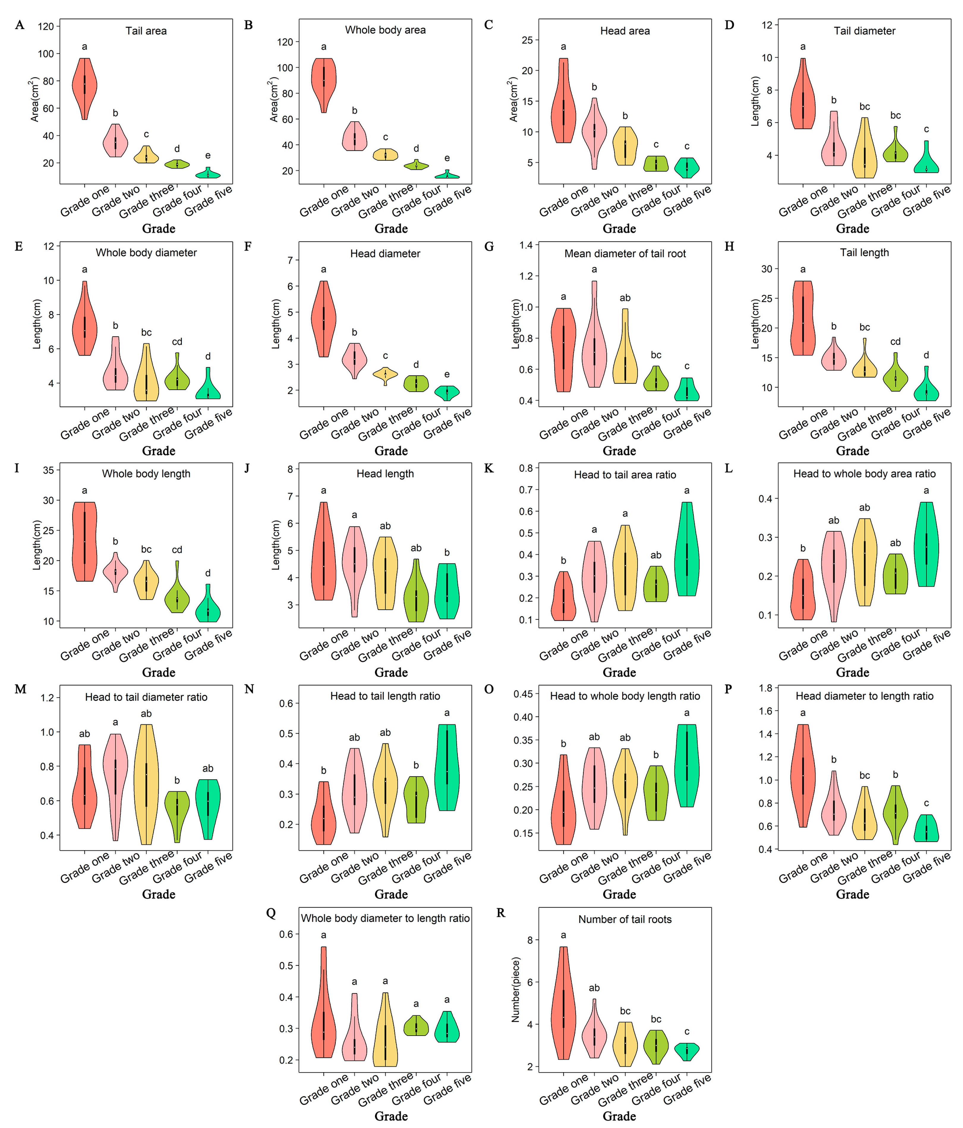
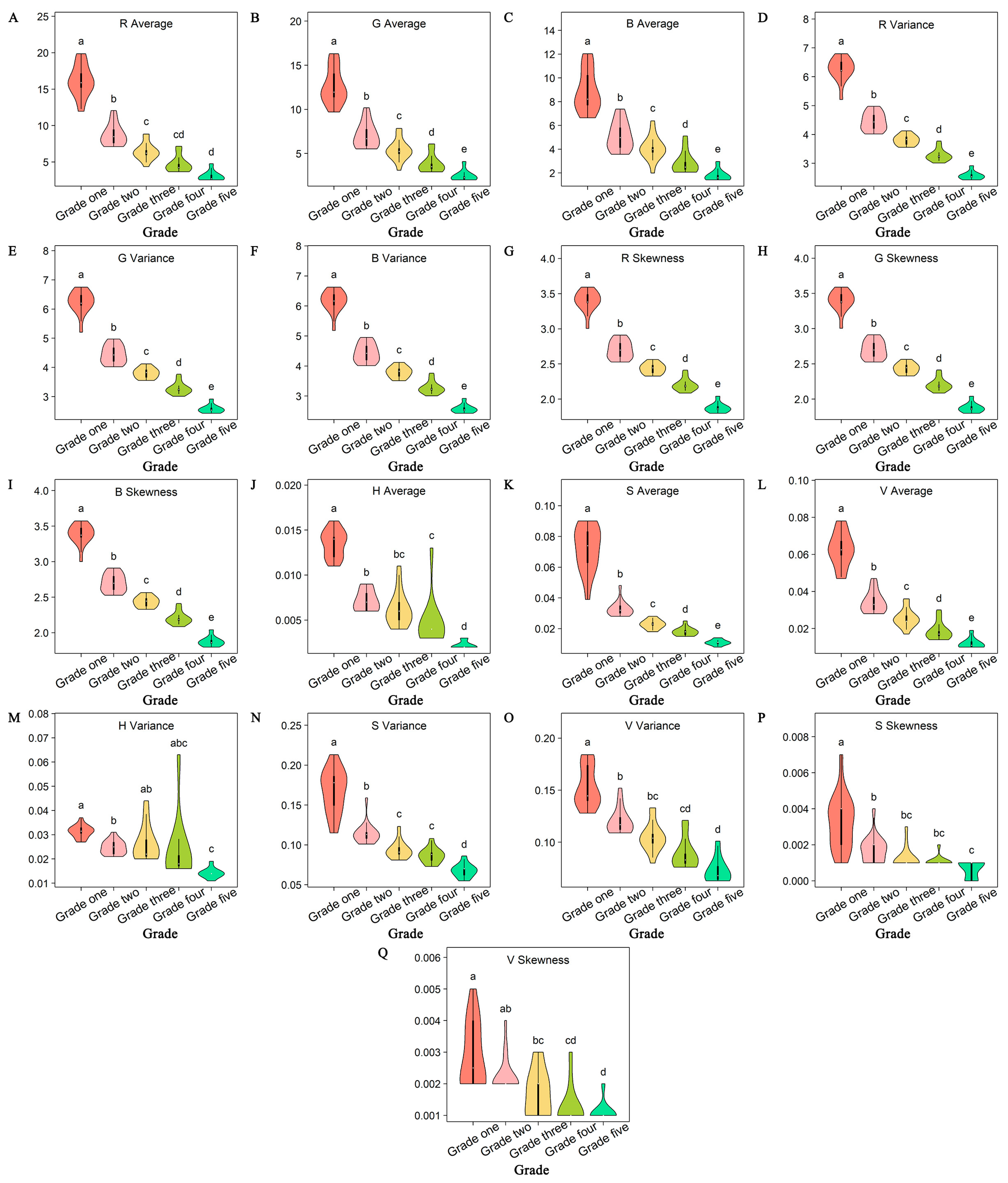
3.1.1. Difference Analysis of Appearance Feature Parameters among Different Grades

The multiple comparison results for 18 shape feature parameters of AS among different grades are shown in Figure 9.

From Figure 9, it can be seen that three shape feature parameters showed significant differences between any two grades, including tail area (Figure 9A), whole body area (Figure 9B), and head diameter (Figure 9F). Conversely, the remaining 15 shape feature parameters did not meet the condition of significant differences between any two grades, including head area, tail diameter, whole body diameter, head length, tail length, whole body length, head to tail area ratio, head to whole body area ratio, head to tail diameter ratio, head to tail length ratio, head to whole body length ratio, head diameter to length ratio, whole body diameter to length ratio, average tail diameter, and the number of tail roots (Figure 9).

The multiple comparison results for 17 color feature parameters of AS among different grades are shown in Figure 10.

From Figure 10, it can be seen that ten color feature parameters showed significant differences between any two grades, including G average (Figure 10B), B average (Figure 10C), R variances (Figure 10D), G variances (Figure 10E), B variances (Figure 10F), R skewness (Figure 10G), G skewness (Figure 10H), B skewness (Figure 10I), S average (Figure 10K), and V average (Figure 10L). Conversely, the remaining seven color feature parameters, specifically the R average, H average, H variances, S variances, V variances, S skewness, and V skewness, did not meet the condition of significant differences between any two grades.

In summary, the feature parameters that showed significant differences between any two grades include three shape feature parameters (3S: tail area, whole body area, and head diameter) and ten color feature parameters (10C: G average, B average, R variances, G variances, B variances, R skewness, G skewness, B skewness, S average, and V average).

3.1.2. Correlation Analysis

In order to determine key appearance feature parameters that distinguish the grades of AS, we analyzed the correlation between AS grades and 13 appearance feature parameters that showed significant differences between any two grades. AS grades, categorized as first through fifth, were numerically denoted as 1, 2, 3, 4, and 5. All feature parameters underwent standardization to eliminate dimensional influence during correlation calculation. The standardization method entailed subtracting the mean and dividing by the standard deviation.

Spearman correlation analysis, facilitated by SPSS 26.0 statistical software, was used to scrutinize the correlation between the 13 appearance feature parameters of AS and its grades. Correlation analysis results (

Table 2. Correlation coefficient between appearance feature parameters and grades of AS.

Feature Parameters	Correlation Coefficient (r)	Feature Parameters	Correlation Coefficient (r)
Tail area	−0.963 **	G variances	−0.972 **
Whole body area	−0.976 **	B variances	−0.971 **
Head diameter	−0.950 **	R skewness	−0.972 **
G average	−0.929 **	G skewness	−0.972 **
B average	−0.905 **	B skewness	−0.972 **
R variances	−0.972 **	S average	−0.968 **
V variances	−0.939 **

Note: ** represented p < 0.01 (two-tailed test).

) revealed a significant negative correlation between the 13 appearance feature parameters of AS and its grades (r < 0, p < 0.01). In simpler terms, higher values of the 13 appearance feature parameters corresponded to lower grades. Notably, the correlation between whole body area and grades stood out as the strongest (r = 0.976). This result aligned with the traditional understanding that a larger size of AS correlates with better quality.

3.1.3. Comprehensive Analysis

Three shape feature parameters (i.e., tail area, whole body area, and head diameter) and ten color feature parameters (i.e., G average, B average, R variances, G variances, B variances, R skewness, G skewness, B skewness, S average, and V average) exhibited statistically significant differences between any two grades and demonstrated a strong correlation with grades. Therefore, these feature parameters were selected for the classification of AS grades based on AS images.

3.2. Classification of AS Grades

3.2.1. Determination of the Optimal Number of Hidden Neurons

In this study, the hidden number empirical formula as well as the trial and error method were used to determine the number of hidden neurons using Equation (21):

$$n=\sqrt{a+b} +c$$

(21)

where n indicated the number of hidden neurons, a indicated the number of input nodes, b indicated the number of output nodes, and c was an integer between 1 and 10.

Using the BPNN model, training was conducted with different numbers of hidden neurons, based on three shape feature parameters (3S), ten color feature parameters (10C), and the combined thirteen feature parameters (13CS). Since not all 13 appearance feature parameters (13CS) were necessarily the best features, this study also used three shape feature parameters (3S) and ten color feature parameters (10C) as two types of features for training and testing. The results of training accuracy with different numbers of hidden neurons are shown in

Table 3. Training accuracy of different number of hidden neurons.

Features	Number of Hidden Neurons	Training Accuracy (%)	Number of Hidden Neurons	Training Accuracy (%)
3S	3	69.9%	8	76.4%
	4	75.5%	9	74.3%
	5	72.3%	10	77.1%
	6	73.2%	11	76.5%
	7	75.1%	12	74.9%
10C	4	62.5%	9	62.0%
	5	57.9%	10	56.6%
	6	60.0%	11	53.4%
	7	60.9%	12	56.0%
	8	60.9%	13	59.7%
13CS	5	85.3%	10	90.0%
	6	87.7%	11	87.2%
	7	90.3%	12	89.3%
	8	87.5%	13	88.4%
	9	90.2%	14	86.8%

Note: 3S represented three shape feature parameters (i.e., tail area, whole body area, and head diameter); 10C were ten color feature parameters (i.e., G average, B average, R variances, G variances, B variances, R skewness, G skewness, B skewness, S average, and V average); 13CS represented the combination of three shape feature and ten color feature parameters.

. For different input parameters, the optimal number of hidden neurons of 3S, 10C, and 13CS was 10, 4 and 7, respectively, and the corresponding accuracies were 77.1%, 62.5%, and 90.3% (Table 3). Therefore, the number of hidden neurons for the input cases of 3S, 10C, and 13CS was defined as 10, 4, and 7, respectively. To compare the effectiveness of the BPNN and GOBPNN models, the number of hidden nodes for both models was set to the same value.

3.2.2. Determination of the Optimal Feature

To determine which kind of feature is the best among 3S, 10C, and 13CS, BPNN and GOBPNN with the optimal number of hidden neurons were used to train and test these three kinds of features. The training accuracy and testing accuracy were illustrated in Figure 11 and

Table 4. The training time and testing time of BPNN and GOBPNN based on different kinds of features.

Model	Feature	Training Time (s)	Testing Time (s)
BPNN	3S	0.615	0.017
	10C	0.648	0.014
	13CS	1.639	0.016
GOBPNN	3S	603.717	0.016
	10C	474.880	0.015
	13CS	678.454	0.015

.

For the training process, regardless of which model was used, 13CS as an input feature had the best recognition effect (accuracy higher than 90%), 10C had the worst recognition effect (accuracy less than 70%), and 3S was in the middle (Figure 11A). The results suggested that the simultaneous use of the three shape feature parameters and the ten color feature parameters could relatively accurately distinguish different grades of AS. Both shape and color were essential factors for grading AS. This was due to the significant variations in grades observed in AS grown in different soil types [36]. Various factors, including soil type, structure, moisture content, nutrient distribution, oxygen levels, environmental pressure, and adaptation mechanisms, impacted the shape of AS [37,38]. And soil mineral content, pH levels, and microbial activity played a role in determining its color [39]. The combination of these factors contributed to the diversity of AS grades. Notably, the contribution of shape features surpassed that of color features. This may be because the differences in shape feature parameters among different grades were higher than the differences in color feature parameters among different grades, which can be seen from the basis of AS grade division [9]. When training the same model, the three input features lasted approximately the same time (Table 4). The test result was generally similar to the training result (Figure 11B). Therefore, 13CS was selected as the input feature for further research.

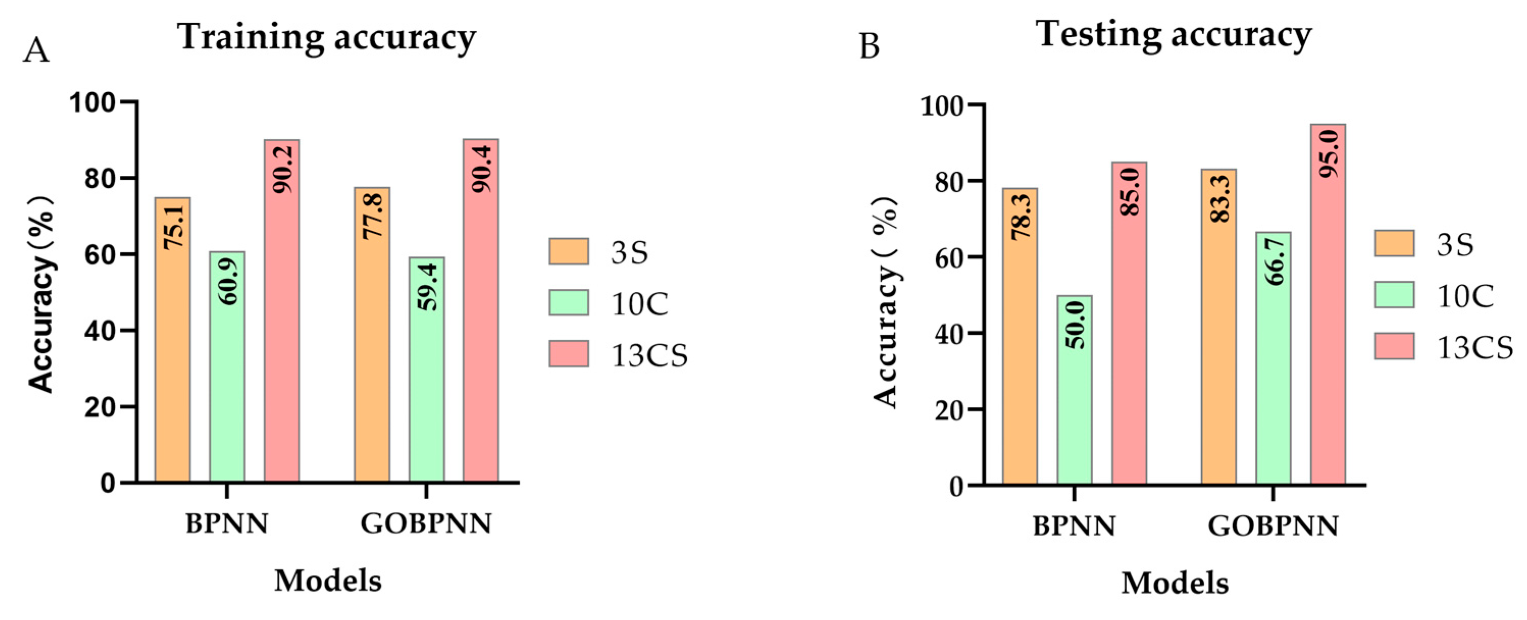
3.2.3. Determination of the Optimal Model

To determine if the improved BPNN (GOBPNN) model has better grade recognition performance than the traditional BPNN model, this study conducted training and testing for AS grade recognition using BPNN and GOBPNN with 13CS as the feature. The testing results are shown in Figure 12 and

Table 5. The testing results of BPNN and GOBPNN at five grades.

Model	Evaluation Index	Grade One	Grade Two	Grade Three	Grade Four	Grade Five	Average Value	Average Growth
BPNN	Precision (%)	83.3	87.5	75.0	66.7	100.0	82.5
	Recall (%)	100.0	95.5	75.0	66.7	78.6	83.2
	F-score (%)	90.9	91.3	75.0	66.7	88.0	82.4
	Accuracy (%)	85.0
GOBPNN	Precision (%)	100.0	91.7	93.8	100.0	100.0	97.1	17.7
	Recall (%)	100.0	100.0	88.2	100.0	91.7	95.9	15.4
	F-score (%)	100.0	95.7	90.9	100.0	95.7	96.5	17.1
	Accuracy (%)	95.0						11.8

.

Based on Figure 12A, the classification of AS by the BPNN model revealed that all tests in grade one AS were accurate. In grade two AS, 95.5% of images were accurately judged, with only one image incorrectly classified as grade three AS. In grade three AS, three-quarters of the images were correctly judged, with three images and one image incorrectly classified as grade two and grade four, respectively. In grade four AS, 66.7% of images were correctly judged, with a few incorrectly classified as grade three (33.3%). In grade five AS, 78.6% of images were correctly judged, with images incorrectly classified as grade one and grade three accounting for 7.1% and 14.3%, respectively.

Based on Figure 12B, it was evident that the classification of AS images using the GOBPNN model yielded accurate results across grades one, two, and four. In grade three AS, only 11.8% of images were erroneously classified as grade two, while in grade five AS, only 8.3% of images were misclassified as grade three.

It was evident that the GOBPNN exhibited superior performance, particularly in substantially enhancing the recognition accuracy of grade four AS. Perhaps due to the tendency of grade four AS samples to fall into local minima in the BPNN model, GOBPNN can effectively solve this problem, thus greatly improving its accuracy.

It can also be seen from Table 5 that GOBPNN achieved higher average precision (97.1%), recall (95.9%), F-score (96.5%), and accuracy (95.0%), while the average precision, recall, F-score, and accuracy for BPNN were 82.5%, 83.2%, 82.4%, and 85.0%, respectively. Notably, compared to BPNN, GOBPNN increased precision, recall, F-score, and accuracy by 17.7%, 15.4%, 17.1%, and 11.8%, respectively. These results indicated that the method based on a computer vision system combined with GOBPNN had proven to be effective in classifying the grades of AS. Compared to traditional empirical identification, this method effectively inherited its convenience, non-destructiveness to samples, and timely conclusions. Additionally, it avoided the drawbacks of non-quantifiable indicators, subjective results, and difficulties in inheritance.

In terms of recognition performance, the results of this study proved to be more effective than those of the recognition of ginseng grades based on images, which had an accuracy of only 74% [20]. In addition, the classification results of this work turned out to be better than the results of the grade identification of the Cornus officinae based on the analysis of color features, using discrimination analysis, least squares support vector machine, and partial least squares discriminant analysis, where the accuracies of the assessment were 86.21%, 89.66%, and 89.66%, respectively [40]. The results of this study were comparable to the results of rhubarb grade recognition based on color features and the BPNN model, where the highest accuracy was 92.3% [22].

From the perspective of time and economic cost, the training time for BPNN and GOBPNN in this study did not exceed 15 min, and the testing time was less than 1 s. It only required taking a photo to obtain the results, which was extremely simple, fast, and cheap. However, through the classification of chemical components, it took several hours just to dissolve powder and extract chemical components, not to mention the time and money used in the long, fumbling conditions to detect chemical component content. Moreover, this method also had other advantages: (1) It could quantify evaluation parameters, making the results relatively objective; (2) the results were stable and not influenced by different evaluators; (3) it did not require damaging AS; (4) the method could be quickly mastered without requiring a long learning period. Based on the above analysis, it can be concluded that the method proposed in this study, which combined machine vision technology with the GOBPNN model, was a convenient and promising approach for classifying the grades of AS.

The training duration of the proposed GOBPNN model in this study may be somewhat prolonged. Future research endeavors could investigate approaches to mitigate model training time or explore alternative models with superior performance to enhance the discrimination of AS grades. Furthermore, the 13 selected feature parameters (tail area, whole body area, head diameter, G average, B average, R variances, G variances, B variances, R skewness, G skewness, B skewness, S average, and V average) identified in this study possess significant value; they can be used for estimating the weight of irregularly shaped AS from images and for researching and refining the quality standards of AS.

4. Conclusions

In this study, we first obtained images of AS at five commodity grades and extracted 19 shape feature parameters, 18 color feature parameters, and eight texture feature parameters from the images. Then, through difference analysis and correlation analysis, we selected three shape feature parameters and 10 color feature parameters for image recognition of AS grades. In order to accurately classify AS grades, the traditional BPNN model was optimized using a growing optimizer (GO). The modeling results showed that the GOBPNN model achieved the highest classification efficiency, expressed as average test precision, recall, F-score and accuracy, amounting to 97.1%, 95.9%, 96.5%, and 95.0%, respectively. Compared to the traditional BPNN model, GOBPNN increased the average test precision, recall, F-score, and accuracy by 17.7%, 15.4%, 17.1%, and 11.8%, respectively. The results indicated that the method combining machine vision technology with GOBPNN enabled efficient, objective, fast, non-destructive, and low-cost classification of the grades of AS, which could help consumers and market regulatory authorities quickly and accurately identify the grade of AS when purchasing it.

References

1. Batiha, G.E.; Shaheen, H.M.; Elhawary, E.A.; Mostafa, N.M.; Eldahshan, O.A.; Sabatier, J. Phytochemical Constituents, Folk Medicinal Uses, and Biological Activities of Genus Angelica: A Review. Molecules 2023, 28, 267. [Google Scholar] [CrossRef]
2. Commission, C.P. Pharmacopoeia of the People’s Republic of Chin 1; China Medical Science and Technology Press: Beijing, China, 2020; p. 1902. ISBN 978-7-5214-1574-2. [Google Scholar]
3. Long, Y.; Li, D.; Yu, S.; Shi, A.; Deng, J.; Wen, J.; Li, X.Q.; Ma, Y.; Zhang, Y.L.; Liu, S.Y.; et al. Medicine–food herb:Angelica sinensis, a potential therapeutic hope for Alzheimer’s disease and related complications. Food Funct. 2022, 13, 8783–8803. [Google Scholar] [CrossRef]
4. Yang, M.J.; Wang, Y.G.; Liu, X.F.; Wu, J.; Qian, J.L. Study on Angelica sinensis Endophytic Fungi and its Antibacterial Activity. Adv. Mater. Res. 2013, 641, 816–819. [Google Scholar] [CrossRef]
5. Xu, S.; Wan, H.; Zhao, X.; Zhang, Y.; Yang, J.; Jin, W.; He, Y. Optimization of extraction and purification processes of six flavonoid components from Radix Astragali using BP neural network combined with particle swarm optimization and genetic algorithm. Ind. Crop. Prod. 2022, 178, 114556. [Google Scholar] [CrossRef]
6. Bi, S.J.; Fu, R.J.; Li, J.J.; Chen, Y.Y.; Tang, Y.P. The Bioactivities and Potential Clinical Values of Angelica Sinensis Polysaccharides. Nat. Prod. Commun. 2021, 16, 1934578X2199732. [Google Scholar] [CrossRef]
7. Nai, J.; Zhang, C.; Shao, H.; Li, B.; Li, H.; Gao, L.; Dai, M.; Zhu, L.; Sheng, H. Extraction, structure, pharmacological activities and drug carrier applications of Angelica sinensis polysaccharide. Int. J. Biol. Macromol. 2021, 183, 2337–2353. [Google Scholar] [CrossRef]
8. Qu, Y.; Liu, H.S.; Hu, J.J.; Zhang, B.H. Study on Commercial Specification Grades Standard and Quality Evaluation of Momordica cochinchinensis. Shi Zhen Chin. Med. 2022, 33, 238–243. [Google Scholar]
9. T/CACM 1021.5-2018; Commercial Grades for Chinese Materia Medica Angelica sinensis Radix. Chinese Association of Traditional Chinese Medicine: Hongkong, China, 2018.
10. Raki, H.; Aalaila, Y.; Taktour, A.H.; Peluffo-Ordóñez, D. Combining AI Tools with Non-Destructive Technologies for Crop-Based Food Safety: A Comprehensive Review. Foods 2024, 13, 11. [Google Scholar] [CrossRef]
11. Xin, N.; Luo, C.; Mo, Y. Comparison of ferulic acid content in different grades of Angelica sinensis. J. Chin. Med. Mater. 2001, 4, 244–245. [Google Scholar] [CrossRef]
12. Zhao, W. Study on the Correlation between the Commercial Specification Grades and Quality of Gansu Angelica Sinensis Radix; Gansu University of Chinese Medicine: Lan Zhou, China, 2018. [Google Scholar]
13. Ruan, H.; Liu, X.; Song, P.; Zhao, D.; Zhao, J.; Yong-Hui, D.; Lu, J.; Lin, R. Rational analysis of Angelica product grades divided by chemical and weight indicators. Chin. J. Tradit. Chin. Med. 2013, 28, 2453–2456. [Google Scholar]
14. Ewa, R.; Justyna, S. The Estimation of Chemical Properties of Pepper Treated with Natural Fertilizers Based on Image Texture Parameters. Foods 2023, 12, 2123. [Google Scholar] [CrossRef]
15. Kakani, V.; Nguyen, V.H.; Kumar, B.P.; Kim, H.; Pasupuleti, V. A critical review on computer vision and artificial intelligence in food industry. J. Agric. Food Res. 2020, 2, 100033. [Google Scholar] [CrossRef]
16. Ding, H.; Tian, J.; Yu, W.; Wilson, D.; Young, B.; Cui, X.; Xin, X.; Wang, Z.; Li, W. The Application of Artificial Intelligence and Big Data in the Food Industry. Foods 2023, 12, 4511. [Google Scholar] [CrossRef]
17. Liu, C.; Wang, Q.; Ma, M.; Zhu, Z.; Lin, W.; Liu, S.; Fan, W. Single-View Measurement Method for Egg Size Based on Small-Batch Images. Foods 2023, 12, 936. [Google Scholar] [CrossRef]
18. Zhao, S.; Bai, Z.; Wang, S.; Gu, Y. Research on Automatic Classification and Detection of Mutton Multi-Parts Based on Swin-Transformer. Foods 2023, 12, 1642. [Google Scholar] [CrossRef]
19. Zhou, W.; Song, C.; Song, K.; Wen, N.; Sun, X.; Gao, P. Surface Defect Detection System for Carrot Combine Harvest Based on Multi-Stage Knowledge Distillation. Foods 2023, 12, 793. [Google Scholar] [CrossRef]
20. Kim, S.M.; Kim, C.S.; Lee, C.H.; Kim, M.H.; Park, S.J. Nondestructive Evaluation System for White Ginseng Quality Using Image Processing Technique. Key Eng. Mater. 2006, 321, 1225–1228. [Google Scholar] [CrossRef]
21. Cui, Y.; Liu, R.; Lin, Z.; Chen, P.; Wang, L.; Wang, Y.; Chen, S. Quality evaluation based on color grading: Quality discrimination of the Chinese medicine Corni Fructus by an E-eye. Sci. Rep. 2019, 9, 17006. [Google Scholar] [CrossRef]
22. Wang, J.; Zeng, L.; Zang, Q.; Gong, Q.; Li, B.; Zhang, X.; Chu, X.; Zhang, P.; Zhao, Y.; Xiao, X.; et al. Colorimetric grading scale can promote the standardization of experiential and sensory evaluation in quality control of traditional Chinese medicines. PLoS ONE 2012, 7, e48887. [Google Scholar] [CrossRef]
23. Zhu, Y.; Zhang, F.; Li, L.; Lin, Y.; Zhang, Z.; Shi, L.; Tao, H.; Qin, T. Research on Classification Model of Panax notoginseng Taproots Based on Machine Vision Feature Fusion. Sensors 2021, 21, 7945. [Google Scholar] [CrossRef]
24. She, B.; Hu, J.; Huang, L.; Zhu, M.; Yin, Q. Mapping Soybean Planting Areas in Regions with Complex Planting Structures Using Machine Learning Models and Chinese GF-6 WFV Data. Agriculture 2024, 14, 231. [Google Scholar] [CrossRef]
25. Li, C.; Wang, X.; Chen, L.; Zhao, X.; Li, Y.; Chen, M.; Liu, H.; Zhai, C. Grading and Detection Method of Asparagus Stem Blight Based on Hyperspectral Imaging of Asparagus Crowns. Agriculture 2023, 13, 1673. [Google Scholar] [CrossRef]
26. Mcclelland, J.; Rumelhart, D. Parallel Distributed Processing; MIT Press: Cambridge, MA, USA, 1986. [Google Scholar]
27. Li, C.H.; Park, S.C. Combination of modified BPNN algorithms and an efficient feature selection method for text categorization. Inf. Process. Manag. 2009, 45, 329–340. [Google Scholar] [CrossRef]
28. Khan, A.; Bukhari, J.; Bangash, J.I.; Khan, A.; Imran, M.; Asim, M.; Ishaq, M.; Khan, A. Optimizing connection weights of functional link neural network using APSO algorithm for medical data classification. J. King Saud Univ. Comput. Inf. Sci. 2022, 34, 2551–2561. [Google Scholar] [CrossRef]
29. Zhang, Q.; Gao, H.; Zhan, Z.; Li, J.; Zhang, H. Growth Optimizer: A powerful metaheuristic algorithm for solving continuous and discrete global optimization problems. Knowl. Based Syst. 2023, 261, 110206. [Google Scholar] [CrossRef]
30. Deng, J.; Zhou, H.; Lv, X.; Yang, L.; Shang, J.; Sun, Q.; Zheng, X.; Zhou, C.; Zhao, B.; Wu, J.; et al. Applying convolutional neural networks for detecting wheat stripe rust transmission centers under complex field conditions using RGB-based high spatial resolution images from UAVs. Comput. Electron. Agric. 2022, 200, 107211. [Google Scholar] [CrossRef]
31. Singh, S.; Mittal, N.; Singh, H.; Oliva, D. Improving the segmentation of digital images by using a modified Otsu’s between-class variance. Multimed. Tools Appl. 2023, 82, 40701–40743. [Google Scholar] [CrossRef]
32. Chen, Y.; Li, Q.; Qiu, D. The Dynamic Accumulation Rules of Chemical Components in Different Medicinal Parts of Angelica sinensis by GC-MS. Molecules 2022, 27, 4617. [Google Scholar] [CrossRef]
33. Chen, L.; Zhu, Y.; Papandreou, G.; Schroff, F.; Adam, H. Encoder-Decoder with Atrous Separable Convolution for Semantic Image Segmentation. In Proceedings of the European Conference on Computer Vision, Munich, Germany, 8–14 September 2018. [Google Scholar]
34. Tamura, H.; Mori, S.; Yamawaki, T. Textural Features Corresponding to Visual Perception. IEEE Trans. Syst. Man Cybern. 1978, 8, 460–473. [Google Scholar] [CrossRef]
35. Rafi, M.; Mukhopadhyay, S. Texture description using multi-scale morphological GLCM. Multimed. Tools Appl. 2018, 77, 30505–30532. [Google Scholar] [CrossRef]
36. Zhu, L.; Yan, H.; Zhou, G.; Jiang, C.; Liu, P.; Yu, G.; Guo, S.; Wu, Q.; Duan, J. Insights into the mechanism of the effects of rhizosphere microorganisms on the quality of authentic Angelica sinensis under different soil microenvironments. Bmc Plant Biol. 2021, 21, 285. [Google Scholar] [CrossRef]
37. Ogilvie, C.M.; Ashiq, W.; Vasava, H.B.; Biswas, A. Quantifying Root-Soil Interactions in Cover Crop Systems: A Review. Agriculture 2021, 11, 218. [Google Scholar] [CrossRef]
38. Borden, K.A.; Anglaaere, L.C.N.; Owusu, S.; Martin, A.R.; Buchanan, S.W.; Addo-Danso, S.D.; Isaac, M.E. Soil texture moderates root functional traits in agroforestry systems across a climatic gradient. Agric. Ecosyst. Environ. 2020, 295, 106915. [Google Scholar] [CrossRef]
39. Ling, L.; Ma, W.; Li, Z.; Jiao, Z.; Xu, X.; Lu, L.; Zhang, X.; Feng, J.; Zhang, J. Comparative study of the endophytic and rhizospheric bacterial diversity of Angelica sinensis in three main producing areas in Gansu, China. S. Afr. J. Bot. 2020, 134, 36–42. [Google Scholar] [CrossRef]
40. Cui, Y.; Wang, L.; Duan, L.; Chen, S. Quality evaluation based on color grading—Relationship between chemical susbtances and commercial grades by machine version in Corni fructus. Trop. J. Pharm. Res. 2020, 19, 1495–1501. [Google Scholar] [CrossRef]
Figure 1. Original images of AS samples at five grades. The five images from left to right represent grade one, grade two, grade three, grade four, and grade five, respectively.
Agriculture 14 00507 g001
Figure 2. Structure diagram of image acquisition system.
Agriculture 14 00507 g002
Figure 3. Diagram of the head, tail, and whole body of AS. The portion inside the red box was the head of AS. The portion inside the green box was the tail of AS. The head and tail together formed the whole body of AS. Each branch of the AS tail was referred to as a tail root of AS.
Agriculture 14 00507 g003
Figure 4. Labeled images for training semantic segmentation model. (A) AS image; (B) the first labeled image; (C) the second labeled image.
Agriculture 14 00507 g004
Figure 5. Semantic recognition effect of AS head, tail, and each root. (A) Original image; (B) manually labeled images of AS head and tail; (C) model prediction result of AS head and tail; (D) manually labeled image of each root of AS; (E) prediction result of the second labeled image.
Agriculture 14 00507 g005
Figure 6. Procedure for extracting the diameter, length, and area of the head, tail, and whole body of AS. (A) The original image; (B) semantic segmentation image of the head (green section) and tail (yellow section) of AS; (C) gray-level image; (D) the pixel gray level of the AS head was set to 255; (E) binary image of the AS head; (F) minimum bounding rectangle of the AS head; (G) the pixel gray level of the AS tail was set to 255; (H) binary image of the AS tail; (I) minimum bounding rectangle of the AS tail; (J) the pixel gray level of the whole body of AS was set to 255; (K) binary image of the whole body of AS; (L) minimum bounding rectangle of the whole body of AS.
Agriculture 14 00507 g006
Figure 7. Procedure of extraction of the number and average diameter of the tail roots of AS. (A) The original image; (B) semantic segmentation image of the tail roots of AS; (C) gray-level image; (D) binary image; (E) minimum bounding rectangle of the entity of tail roots; (F) a horizontal line at the upper quarter of this rectangle in the vertical direction; (G) overlap between the horizontal line and the tail roots.
Agriculture 14 00507 g007
Figure 8. Flowchart of the GOBPNN model.
Agriculture 14 00507 g008
Figure 9. Differences in 18 shape feature parameters among different grades of AS. Note: abcde represent different levels of significance. Different letters indicate significant differences, while the same letter implies no significant difference.
Agriculture 14 00507 g009
Figure 10. Differences in 17 color feature parameters among different grades of AS. Note: abcde represent different levels of significance. Different letters indicate significant differences, while the same letter implies no significant difference.
Agriculture 14 00507 g010
Figure 11. Training (A) and testing (B) accuracy of BPNN and GOBPNN based on different kinds of features.
Agriculture 14 00507 g011
Figure 12. The confusion matrix for BPNN and GOBPNN. (A) BPNN confusion matrix; (B) GOBPNN confusion matrix. Note: 1, 2, 3, 4, and 5, respectively, represent grades one, two, three, four, and five of AS.
Agriculture 14 00507 g012