Multi-Trait Bayesian Models Enhance the Accuracy of Genomic Prediction in Multi-Breed Reference Populations


1
State Key Laboratory of Animal Biotech Breeding, College of Animal Science and Technology, China Agricultural University, Haidian, Beijing 100193, China
2
Beijing Zhongyu Pig Breeding Co., Ltd., Beijing 100194, China
*
Author to whom correspondence should be addressed.
Agriculture 2024, 14(4), 626; https://doi.org/10.3390/agriculture14040626
Submission received: 9 March 2024
/
Revised: 10 April 2024
/
Accepted: 16 April 2024
/
Published: 18 April 2024
(This article belongs to the Section Farm Animal Production)
Abstract
:Performing joint genomic predictions for multiple breeds (MBGP) to expand the reference size is a promising strategy for improving the prediction for limited population sizes or phenotypic records for a single breed. This study proposes an MBGP model—mbBayesAB, which treats the same traits of different breeds as potentially genetically related but different, and divides chromosomes into independent blocks to fit heterogeneous genetic (co)variances. Best practices of random effect (co)variance matrix priors in mbBayesAB were analyzed, and the prediction accuracies of mbBayesAB were compared with within-breed (WBGP) and other commonly used MBGP models. The results showed that assigning an inverse Wishart prior to the random effect and obtaining information on the scale of the inverse Wishart prior from the phenotype enabled mbBayesAB to achieve the highest accuracy. When combining two cattle breeds (Limousin and Angus) in reference, mbBayesAB achieved higher accuracy than the WBGP model for two weight traits. For the marbling score trait in pigs, MBGP of the Yorkshire and Landrace breeds led to a 6.27% increase in accuracy for Yorkshire validation using mbBayesAB compared to that using the WBGP model. Therefore, considering heterogeneous genetic (co)variance in MBGP is advantageous. However, determining appropriate priors for (co)variance and hyperparameters is crucial for MBGP.
1. Introduction
Genome prediction (GP) estimates genome breeding values (GEBVs) using genetic markers (usually single-nucleotide polymorphisms [SNPs]) covering the whole genome [1] and is widely used in animal and plant breeding practices [2]. GP can achieve higher genetic gains than traditional pedigree-based methods for estimating breeding values [3,4]. The accuracy of GP is influenced by factors such as the size and composition of the reference population [5], the relationship between the reference and predicted populations [6], and the genetic structure of the traits [7]. Increasing the number of individuals in the reference group is the most direct and effective method for improving GP accuracy [8]. However, obtaining an ideal GP reference population is challenging due to the high cost of genotyping, the difficulty of phenotyping, and the limited population sizes of some local breeds [9,10].
One way to overcome these limitations is to perform multi-breed genomic prediction (MBGP), in which information from multiple breeds is combined to form a large reference population to improve prediction accuracy [11,12,13,14]. The most direct approach to MBGP is blending individuals from different populations and estimating GEBVs using univariate models, assuming a genetic correlation of one between all breeds. This method has been proven to be effective when merging closely related populations, such as those originating from the same breed [15,16,17]. However, when merging distantly related breeds or populations, this rough processing method does not improve prediction accuracy and may yield lower accuracy than within-breed GP (WBGP) [18,19,20]. Consequently, researchers have attempted to apply multi-trait models for joint prediction, treating same traits from different populations as potentially correlated traits [21,22,23]. By considering their genetic correlations, the multi-trait model offer flexibility in managing populations with diverse genetic backgrounds. This allows for the weighting of information from different breeds according to the estimated genetic correlations to derive the GEBVs of validation individuals. If there is a non-zero genetic correlation between breeds due to common breeding objectives for target traits, information regarding individuals of different breeds within the reference population can be borrowed [24]. Similar to fitting heterogeneous genetic (co)variance in multi-trait models [25,26], allowing for different genetic correlation sizes between breeds in different genomic regions is more reasonable than assuming uniform genetic correlations across the whole genome. This key point is not considered in MBGP, and overestimating or underestimating of local genetic correlations among breeds decreases the prediction accuracy.
The multi-trait Bayesian model provides a flexible solution to the aforementioned problems, allowing the fitting of heterogeneous genetic (co)variance for different genome blocks [27]. Additionally, estimating reliable genetic correlation values for different blocks of the genome increases the accuracy of information sharing among breeds [23]. Owing to its conjugate properties and computational simplicity, the inverse Wishart (IW) distribution is commonly used as a prior for the covariance matrix in multivariate Bayesian models [28]. Researchers usually assume that the degrees of freedom (df) and scale matrix (S) parameters in the IW prior are known, and these are referred to as hyperparameters. In practical analyses, the determination of these hyperparameters significantly affects model performance [29]. The df and S are normally set to p + 1 and the identity p × p matrix Ip, respectively, where p represents the number of traits in multi-trait models [30,31,32]. However, this default parameter setting may affect the accuracy of the inference for posterior distributions [33,34]. Additionally, assuming an IW prior leads to a strong relationship between the variance and correlation, potentially introducing bias into the inference [32]. One solution is to specify a hierarchical inverse Wishart (HIW) prior to the (co)variance matrix of the random effects. That is, assuming that S is unknown but follows a specific distribution, and then obtaining estimates of S from the posterior distribution [29]. The estimation error of the genetic correlation is superimposed with an increase in the number of genome blocks, which significantly decreases the prediction accuracy. Therefore, carefully determining the priors in the model that fit a specific SNP effect (co)variance matrix for different genome blocks is critical.
This study explores whether a multivariate genomic prediction model can improve MBGP. This model treats the same trait from different breeds as different traits with potential genetic correlations while allowing for the variation of genetic correlations between breeds in different genomic blocks. We used two publicly available datasets, including cattle populations comprising Limousin and Angus breeds, and pig populations comprising Yorkshire and Landrace breeds for methods validation. Traits analyzed included marbling score, fat area ratio in the image, yearling weight, and weaning weight. The impact of hyperparameter choices on the IW prior and the model’s performance using an alternative HIW prior to the SNP effect (co)variance matrix was investigated based on real pigs and beef cattle data. This study will confirm the importance of considering heterogeneous genetic (co)variance in MBGP and provide novel insights and perspectives for exploring joint prediction models.
2. Materials and Methods
2.1. Dataset
In many studies, the accuracy of genomic prediction has been reported to vary with population and trait. Therefore, to validate whether the method proposed in this study has advantages in joint prediction, we analyzed real data from two different species (pigs and beef cattle).
2.1.1. Real Pig Data
The real pig dataset used in this study was obtained from Xie et al. [35]. This study used two purebred populations of 228 Landrace (LL, 141 sows and 87 barrows) and 641 Yorkshire (YY, 407 sows and 234 barrows) pigs. All pigs were raised in Muyuan Food Co., Ltd. (Henan, China), which adopts a large-scale intensive raising model. Two traits, marbling score (MS) and fat area ratio in the image (PFAI), were analyzed. PFAI, the digital intramuscular fat content, was calculated using the formula , where the fat area pixel and target area pixel were obtained from digital images of the longissimus dorsi muscle (LDM) slice captured by a digital camera. The MS were provided by members of a professional meat quality scoring team based on LDM slice images. The scoring ranged from 1 (minimum marbling) to 10 (maximum marbling), and the final MS was determined as the average score of those reported by the three team members. All individuals in the dataset had phenotypes and genotypes. Genotyping was performed using the CC1 PorcineSNP50 BeadChip (51,368 SNPs) according to the manufacturer’s protocol. Quality control was performed to exclude SNPs with a call rate of <95% and minor allele frequency of <1%. Following quality control, 37,304 SNPs were retained for subsequent analyses.
2.1.2. Real Beef Cattle Data
The real beef cattle dataset used in this study was obtained from Lee et al. [36]. Two purebred populations, 1907 Limousin (LIM) and 800 Angus (AAN), were used in the analyses. The common traits of yearling weight (YWT) and weening weight (WWT) in beef cattle breeding were analyzed. The phenotypes and genotypes for all individuals were available. All animals were genotyped with the Illumina BovineSNP50 BeadChip, and 54,609 SNP markers were retrieved. Quality control was carried out to exclude SNPs with a call rate of <95% and minor allele frequency of <1%. After quality control, 37,150 SNPs were retained for subsequent analyses.
2.2. Multi-Breed Joint Prediction Model mbBayesAB
To fit the heterogeneity (co)variance of different genomic regions, the following model is proposed:
where is the response variable vector of breed l; b is the fixed effect vector assigned with a uniform prior. In MBGP models, the intercept and breed were included as fixed effects. Additionally, an extra sex fixed effect was added to the analysis of pig data. In the WBGP model, except for the absence of breed fixed effects, the settings are the same as those in the corresponding MBGP models. is the allelic substitution effect of breed l at SNP j in block i; and is the number of SNPs in block i. Unless specified otherwise, each chromosome is divided into blocks based on the number (in 100) of adjacent SNPs. is the SNP effect vector following a multivariate normal distribution. The prior of the SNP in block i is ; is the (co)variance matrix of all the SNP effects in block i, where its prior is the IW distribution ; is a hyperparameter that must be provided, which is often considered an estimate of the value of ; is the residual effect vector of breed l and , where is the (co)variance matrix of the residual effect. According to Bayesian theory, the posterior distribution of these effects and their (co)variance matrix can be derived as
where IW means that the variable follows the inverse Wishart distribution; is the allele content matrix encoded as 0,1,2; is a diagonal matrix in which all diagonal elements equal ; and are vectors of corrected phenotypic values in different scenarios; is the residual effect vector of individual k; n is the total number of individuals in the population being analyzed; and p is the number of breeds.
Determination the hyperparameter df and scale matrix B in the aforementioned model is essential for a posteriori inference. First, df was set as p + 1 [29,30,31], and then the influence of the scale matrix on the model’s performance was studied using different calculation methods based on B. The scale matrix was assumed to be derived from the identity matrix and set to Ip and df × Ip [37]. Because of the small additive genetic variance explained by each SNP in GP, a scale matrix of 0.01 × Ip was used. Additionally, the scale matrix from the phenotypes were obtained, where ; is the prior of heritability (we used 0.5); P is the diagonal matrix with diagonal elements as phenotypic variance; is the allele frequency of SNP j; and m is the total number of SNPs in the analyses. For the residual effects, when the scale matrix information was derived from the identity matrix and its scaled form, the setting value was consistent with that of the SNP effect. When attempting to obtain the scale matrix from the phenotype, was set in our study. The choice of df determines the variance uncertainty in the IW prior [38]. In this study, df was as p, p + 1, p + 2, p + 3, and p + 4. Additionally, because each genome block contains 100 SNPs, the df in the posterior distribution of the SNP effect (co)variance matrix was set to df + 100. Considering that a smaller df may have less impact on posterior inference, the impact of a relatively large df (p + 98) on posterior inference was explored.
Huang and Wand [39] proposed that, compared with the IW prior, specifying a HIW prior for the (co)variance matrix provides high flexibility in selecting the scaling matrix while retaining the conjugate property. Therefore, in this study, two types of HIW priors were used to replace the IW prior, and their application effect in mbBayesAB was explored. First, a Wishart prior to the scale matrix was assigned in the IW prior (HIW-WI) [40]:
where IG indicates that the variable follows an inverse gamma distribution; is a diagonal matrix with diagonal ; A is a sufficiently large integer (we used 105); and the standard deviation of the SNP effect follows a half-t distribution. Additionally, because the scale matrix in IW prior is a diagonal matrix, the marginal distribution of the correlation coefficient was deduced to be ; when , the marginal distribution of the correlation coefficient is uniform [39], and the degree of freedom was set to when specifying a HIW-IG prior for this study.
Second, an inverse gamma prior was assigned to the scale matrix in the IW prior (HIW-IG) [40]:
where WI means that the variable follows the Wishart distribution and and are the known hyperparameters assumed in the model. Mulder and Pericchi (2018) [40] demonstrated that follows the matrix-F distribution , and the marginal distribution obtained under this prior setting has an ideal pole at zero, which is a key characteristic of the horseshoe shape. Appendix A presents the posterior derivation process for the two HIW priors.
Karaman et al. [41] also fitted the heterogeneous genetic (co)variance in a multi-trait Bayesian model and found differences in prediction accuracy when dividing blocks based on different numbers of SNPs. To study the impact of the number of SNPs on the prediction accuracy of mbBayesAB when defining blocks, different SNP number gradients were set: a group of 1, 25, 50, 100, or 200 adjacent SNPs or the whole genome. For the prior assumption of the (co)variance matrix of the random effects in this model, the best parameters determined in our study were used.
All Bayesian models used custom-developed software (https://github.com/CAU-TeamLiuJF/mbBayesAB/bin/mbBayesAB, accessed on 16 April 2024) to obtain the GEBVs. Analyses of the posterior samples indicated that increasing the number of iterations beyond 30,000 led to highly consistent outcomes for different Bayesian models. Therefore, the Gibbs sampler was run for 30,000 cycles, of which the first 20,000 were treated as burned-in, with a thinning interval of 10 cycles.
2.3. Other Models for Comparison with mbBayesAB
Three genomic best linear unbiased prediction (GBLUP) models were fitted to determine whether mbBayesAB is superior to the WBGP and the widely used MBGP models. A single-trait GBLUP model w-GBLUP, whose reference comprises one purebred population. To understand the genetic architecture of the analyzed traits, the w-GBLUP model was also employed to estimate the heritability of the analyzed traits across different breeds. In contrast with w-GBLUP, b-GBLUP uses two purebred populations in the reference and includes an extra breed fixed effect. A multi-trait GBLUP model u-GBLUP views traits belonging to the same breed as distinct but potentially connected. For a comprehensive discussion of the models, see Appendix A.
2.4. Cross-Validation (CV) and Predictive Accuracy
This study used a five-fold CV method to obtain the prediction accuracy of the model. The complete dataset comprised individuals with genotypes and phenotypes, who were then randomly divided into five subgroups of equal sizes. One subset was designated as the validation set and the phenotypic value of the individual was set as missing. The other four subgroups constituted the training set for predicting the GEBVs of the validation individuals. This process was repeated 10 times to reduce random errors. Based on the complete dataset, a corrected phenotypic value (yc) was calculated using the GBLUP model. Predictive accuracy was evaluated by calculating the correlation coefficient between GEBVs and yc of individuals in the validation. In the WBGP model, the individuals in the reference and validation populations belonged to the same breeds. The validation subset used was consistent with the WBGP model for all models, indicating that subgroup division was performed only once.
2.5. Genomic Structure Analysis
The difference in genetic background among breeds is a key factor affecting joint prediction. Therefore, the genetic structure of the population in the analysis dataset was studied based on genotype information. The PLINK software (v1.9) [42] was used to obtain the principal component and linkage disequilibrium (LD) measure r2 based on the genotype data, followed by generation of the corresponding plots. Additionally, the LD consistency between breeds was calculated [43].
3. Results
3.1. Population Genomic Structure and Heritability of Traits
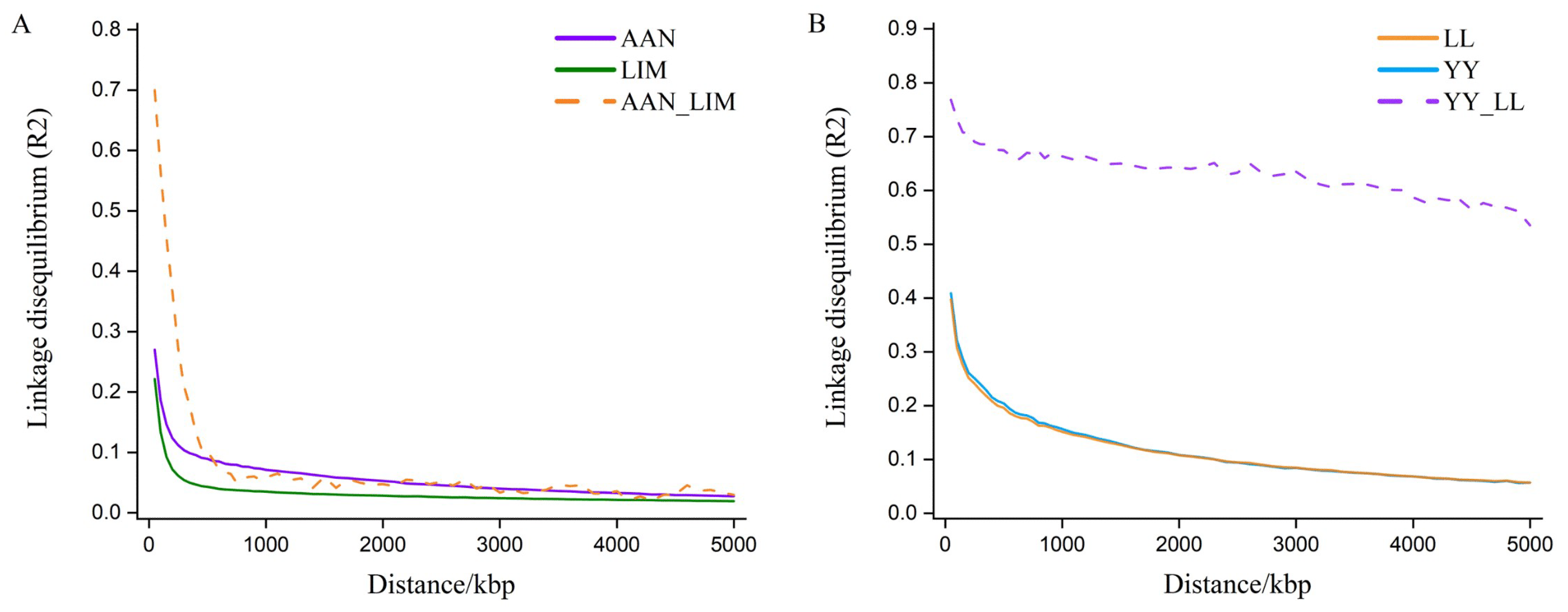
According to the individual dispersion of the first and second principal components (Figure A1), the genetic differences between breeds in the two datasets were significant. In the LD r2 and LD consistency plots (Figure A2), certain differences in the LD patterns were observed between the two datasets. The LD of the two beef cattle breeds decreased faster than that of the pigs at the same distance, and the consistency of the LD among the cattle breeds was lower than that of the pigs. These results indicated that the genetic relationship between LIM and AAN was more distant than that between the two pig breeds. These results showed that the dataset used in this study represents various situations that may exist in MBGP and is suitable for testing the performance of different joint prediction models.
The residual variance estimates for YY and LL were close, and the difference in heritability estimates mainly arose from additive genetic variance (Table 1). Notably, although LL showed higher heritability estimates than YY, the standard error for its heritability was noticeably larger than that of YY. The heritability estimates for the cattle population for YWT and WWT were greater than 0.5. The heritability estimates for the YWT trait differed substantially between LIM and AAN, whereas the estimates for the WWT were similar between the two breeds. Additionally, the standard error of the heritability for both traits was small for LIM and AAN. However, the estimates of additive genetic and residual variance for the WWT trait in LIM and AAN differed by an order of magnitude.
3.2. Degrees of Freedom and Scale Matrix Hyperparameters in IW Prior
The impact of different scale matrix B settings on the prediction accuracy of mbBayesAB was analyzed. The results showed that the estimated value of the scale matrix from the phenotypic information of the analyzed traits achieved the highest prediction accuracy (Figure 1). When an identity matrix and its scaled form, which are generally considered to carry no additional information such as guess values for B, the prediction accuracy was considerably affected. Notably, the prediction accuracy showed an upward trend in most cases when a lower marker effect variance prior was provided. However, even when scaled down to the same order of magnitude as B estimated from the phenotypic data, its prediction accuracy was not as good as that of the latter. The number of pig breeds was smaller than that of beef cattle, which may be one of the reasons because of which the posterior inference of the former was more sensitive than the latter to the choice of the scale matrix.
As the degrees of freedom in the IW prior distribution increase, the amount of information provided by the prior increases [28]. However, when the freedom is too large, posterior inference may be dominated by empirical information and unable to obtain effective information from the real data. The results of analysis of the real data confirmed that extreme degree-of-freedom parameters (too large or too small) adversely affected prediction accuracy (Figure 2). In the joint prediction of the two beef cattle breeds, using df = p + 1 achieved a higher prediction accuracy than that using other settings, and this strategy has been observed in other studies [29,30,31]. However, the analysis of the pig dataset showed that df = p + 3 performed optimally, consistent with the findings of Rossi et al. [44].
3.3. Hierarchical Inverse Wishart Prior
To study whether alternative priors can avoid the adverse effects of IW prior characteristics on posterior inference in multi-breed joint assessment models, we specified hierarchical IW priors for the (co)variance matrix of the labeling effect. The results showed that specifying a Wishart distribution or an inverse gamma distribution for the IW prior-scale matrix does not improve prediction accuracy (Table 2). For the joint prediction results for beef cattle, assigning an HIW prior to the marker effect (co)variance matrix resulted in lower average genetic correlation estimates than that obtained after assigning an IW prior. However, the average genetic correlation estimates between breeds were almost zero for the analysis outputs of different models and datasets.
3.4. Number of SNPs in Genome Block Partitioning
Block size can affect prediction accuracy of single-trait or multi-trait Bayesian models fitting heterogeneous genetic (co)variances [41,45]. In the present study, the prediction accuracy of mbBayesAB for different block sizes (one SNP; a group of 25, 50, 100, 200 adjacent SNPs or the whole genome) was compared. The degree of freedom df was set to p + 3, and the scale parameter in the IW prior was estimated from the phenotype variance. Although none of the block sizes maintained an advantage under all scenarios, block splitting for 50 or 100 adjacent SNPs seemed a good choice (Figure 3). Gianola et al. [46] suggested establishing marker clusters to alleviate the impact of marker effect variance prior to Bayesian inference. However, for analysis of the LL breed, higher prediction accuracy was obtained without marker clustering (i.e., only one SNP in each block) compared to that obtained by grouping adjacent markers into sets of 25, 200, or including all markers in the analysis (paired t-test, p < 0.05). Not performing marker grouping resulted in higher prediction accuracy than grouping adjacent SNPs into sets of 50 and 100; however, the difference was not statistically significant (p > 0.05).
3.5. Prediction Accuracy of mbBayesAB and Commonly Used Joint Prediction Models
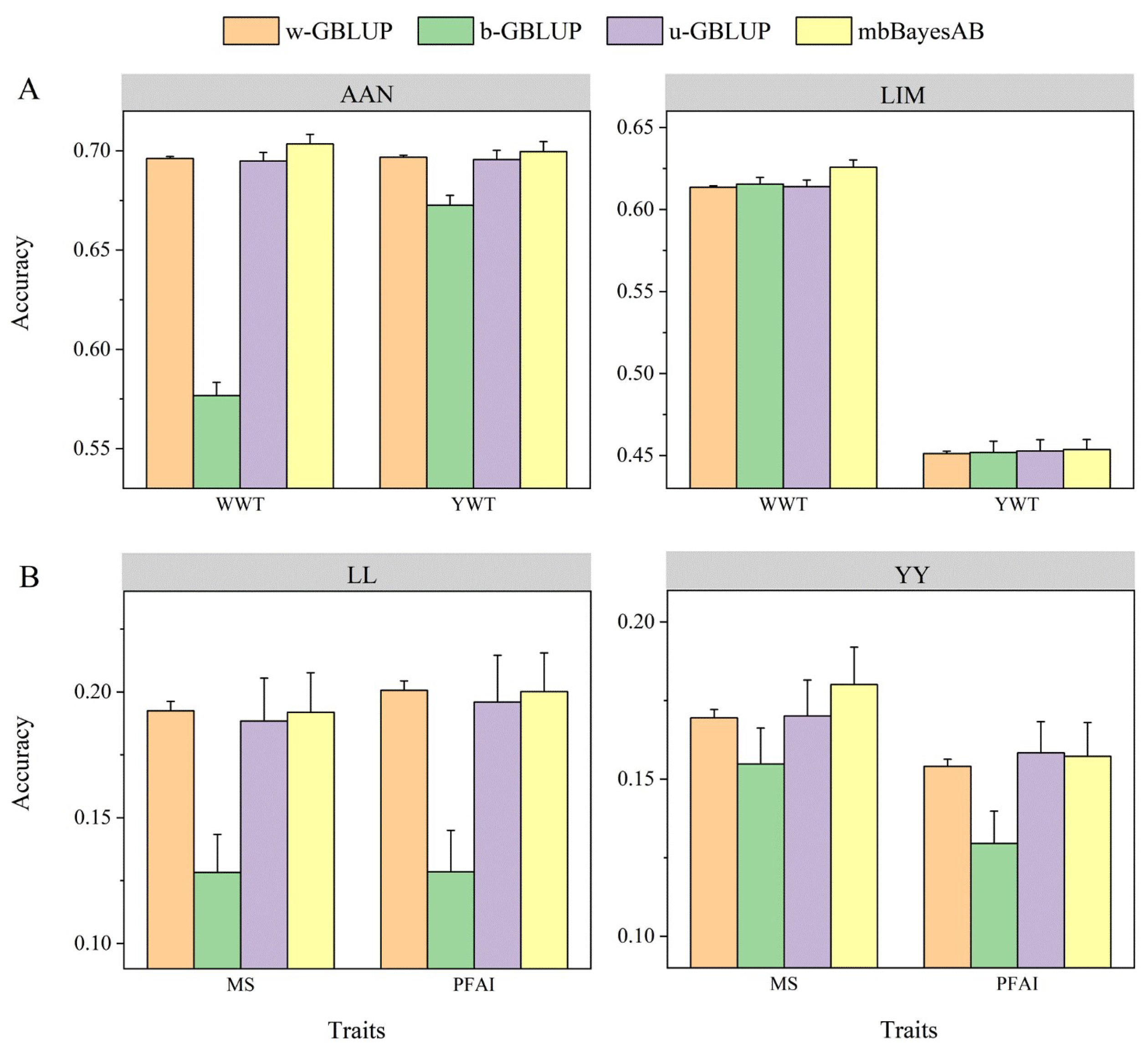
In this study, the optimal parameter settings for the mbBayesAB model were determined. Subsequently, the prediction accuracy of mbBayesAB with that of the WBGP model and the two commonly used MBGP models was compared. The random effects (co)variance matrix in mbBayesAB was set a prior to the IW distribution, and the scale matrix was calculated from the phenotypic variance. In the data analysis of beef cattle and pigs, the df hyperparameters were set to p + 1 and p + 3, respectively. The results showed that the aforementioned parameters achieved high prediction accuracy in the corresponding dataset analysis. In most cases, the mbBayesAB model achieved higher prediction accuracy for both within-breed and multi-breed predictions (Figure 4). Moreover, simply blending data from the two breeds for prediction in a single-trait model yielded a lower prediction accuracy than within-breed prediction. The multi-trait GBLUP model u-GBLUP achieved higher prediction accuracy than its corresponding single-trait form as the model b-GBLUP, indicating the advantages of multi-trait models in joint prediction. When heterogeneous genetic (co)variances were fitted in the MBGP, the model’s prediction accuracy improved, achieving the highest prediction accuracy in most cases.
4. Discussion
Determining of the IW prior hyperparameter is crucial for the posterior inference of the parameters [47]. Zhang [28] demonstrated that the posterior mean is the weighted average of the sample covariance matrix and the prior mean. In the present study, when an identity matrix I for the scale matrix of the IW prior was specified, the posterior inference was adversely affected, and this effect was more evident in pigs with smaller population sizes (Figure 1). The results demonstrate that obtaining a data-dominated parameter value in the absence of sufficient data is difficult if a prior value that is far from the real value for the model parameters is provided. The assignment of degrees of freedom to the IW prior also significantly affected the predictive accuracy of the MBGP model (Figure 2). The larger the degree of freedom parameter df, the higher the certainty of the information in the scale matrix B [28]. However, the results showed that using the value of the degree-of-freedom parameter (df = 2) with the minimum amount of information did not provide any advantage in most cases. The p + 1 degree of freedom used in this study performed optimally for beef cattle data analysis, whereas using p + 3 led to a relatively high predictive accuracy in pigs with smaller population sizes compared to beef cattle. Therefore, when fewer data are available, a reasonable choice is to use df = p + 3. Zhang [28] suggested that the degrees of freedom of the IW prior can be determined from the expression when the variance estimation of the (co)variance matrix is available. However, when the dataset is used twice in the analysis, the certainty of the estimated parameters may be exaggerated. Kass and Steffey [48] showed that specifying an empirical inference value for the prior parameters resulted in a very small posterior variance of the random effects, suggesting that it cannot approach the correct posterior variance through Bayesian learning.
Although the IW prior is widely used in multivariate Bayesian models, it depends on the estimated standard deviation and correlation coefficient. For example, a standard deviation close to zero often appears when the genetic correlation is close to zero [32,49]. In quantitative genetics, quantitative traits are usually controlled by many genes with small effects; therefore, the genetic variance explained by a single genetic marker is small. According to the results of the real data, there was no significant difference in prediction accuracy between specifying the HIW-WI and HIW-IG priors for the marker effect (co)variance matrix and the commonly used IW priors (p < 0.05). However, a serious issue of the IW prior is that precision of all elements in the (co)variance matrix is controlled by a single degree freedom parameter, whereas the HIW prior can help address this defect [50,51]. In our study, the same prior hyperparameters were provided for different breeds, which may be one reason why the HIW prior did not show any advantages in posterior inference. Next, we studied the effect of specifying different hyperparameters for each breed’s marker effect variance on the model’s performance. Additionally, the study predicted that the influence of certain unfavorable characteristics of the IW prior on posterior inference would become more obvious with an increase in the number of elements in the marker effect (co)variance matrix. Therefore, when the number of breeds was increased, the effect of specifying different priors for the (co)variance matrix on the prediction accuracy required further study.
Gianola et al. [46] indicated that forming marker clusters such that their effects have the same variance can reduce the impact of prior on Bayesian inference. Due to their ease of use, it is common practice in multi-trait Bayesian models to group a fixed number of adjacent SNPs together to form marker clusters [41,52]. In this study, the effect of different block sizes (one SNP, a group of 25, 50, 100, or 200 adjacent SNPs, or the whole genome) on the prediction accuracy of the mbBayesAB model was investigated. None of the block sizes exhibited the highest prediction accuracy in all cases. However, a relatively moderate size (50 or 100 SNPs) may be a robust choice, which is consistent with to the block size (100 SNPs) recommended by Gebreyesus et al. [52]. The optimal block size differed among different datasets, which may be a parameter based on a specific genetic background. Genetic information is usually transmitted form parent to offspring in the form of a haplotype; therefore, chromosomes can also be divided into blocks according to their LD information [53].
If the data of multiple breeds were to be directly mixed, and the genomic prediction of the target breed simply based on the fixed effect of the breed, the predictive accuracy may be lower than when using the information of a single breed. This result is consistent with the conclusions of similar studies [54,55], and may be due to the large differences in genetic background among the breeds; however, this simple blending strategy also resulted in noise in the GEBV estimation of both breeds. The multi-trait model provides a new approach for the joint prediction of multiple populations [56,57,58] because it can flexibly manage different genetic relationships. The joint prediction model used in this study allows for different genetic correlation sizes among breeds in different genome blocks, with the result that information sharing among breeds is more accurate than assuming uniform genetic correlations across the whole genome. Additionally, a multi-trait model can effectively process gene–environment interaction effects [59,60], which increases in importance when combining multiple populations for GP. Because these populations are often fed under different environmental conditions, accurately dissecting random environmental effects is conducive to improving prediction accuracy. The estimated value of genetic correlation showed that the global genetic correlation of the genome among breeds was approximately zero; however, there were many blocks in the genome exhibited genetic correlations far from zero. Notably, the data might not be sufficient to accurately estimate the true genetic correlation between breeds owing to zero being the prior value for the correlation between marker effects in all blocks.
The size of the reference population is an important factor influencing prediction accuracy in joint prediction. The population sizes of two beef cattle breeds, LIM (1907) and AAN (800), used in this study were larger than those of the pig breeds, YY (641) and LL (228). Although a higher prediction accuracy was achieved in MBGP of beef cattle populations compared to WBGP, the improvement was relatively small. However, for MS traits, MBGP of the YY and LL breeds resulted in a 6.27% increase in prediction accuracy for individuals in the YY validation. Kjetså et al. [61] demonstrated that adding data of individuals from other breeds to the reference for MBGP could improve prediction accuracy when the population size is small. Therefore, further studies included simulation research and real data analysis should be conducted to improve prediction accuracy. Furthermore, the model will be employed as a multi-trait Bayesian model for joint prediction.
5. Conclusions
Joint genome prediction is crucial for selecting local breeds, developing new traits, and across-county joint evaluation. In this study, a multi-trait Bayesian model was used for multi-breed joint genome prediction and extended to fulfill the needs of heterogeneous genetic (co)variance in different genome blocks. The results demonstrated that mbBayesAB can improve the prediction accuracy of the target breed and obtain a higher prediction accuracy than commonly used joint prediction models. Notably, the choice of priors and assignment of hyperparameters in the model significantly impact the prediction accuracy. Overall, the study proved the effectiveness of a multi-trait Bayesian model in multi-breed joint prediction. However, further research is necessary to accurately estimate local genetic correlations.
Author Contributions
Conceptualization, J.L. and L.Z.; software, W.L.; resources, M.Z.; writing—original draft preparation, W.L.; writing—review and editing, J.W., W.L., L.Z., M.Z. and H.D. All authors have read and agreed to the published version of the manuscript.
Funding
This research was funded by the National Key R&D Program of China (2023ZD0404405), the Earmarked Fund for China Agriculture Research System (No. CARS-pig-35), and the Beijing Municipal Commission of Science and Technology (Z211100004621005).
Institutional Review Board Statement
Not applicable.
Data Availability Statement
The codes and programs needed to reproduce all results in this study are available for download from the following GitHub repository: https://github.com/CAU-TeamLiuJF/mbBayesAB (accessed on 16 April 2024).
Acknowledgments
The authors express their gratitude for the support received from the high-performance computing platform of the National Research Facility for Phenotypic and Genotypic Analysis of Model Animals, and the High-performance Computing Platform of China Agricultural University.
Conflicts of Interest
The authors have read the journal’s guidelines and have the following competing interests: the co-author, J.W., is an employee of Beijing Zhongyu Pig Breeding Co., Ltd. and partially participated in the analysis. The other authors have no competing interests.
Appendix A
The model proposed in this study can be expressed in the following matrix form:
where is the phenotypes (or corrected phenotypes) vector of breed l, b is the vector of fixed effect with a uniform prior; s is the number of blocks across all chromosomes, is the number of SNPs in the ith block; is the allelic substitution effect of breed l at the marker j within the ith block, and it follows a multivariate normal distribution, with the prior of markers’ effect in the ith block being ; is the (co)variance matrix of all marker effects within the block, with a prior of IW distribution ; e is residual effect vector that follows and .
In this study, we assumed that the scale matrix of the random effect prior was unknown and assigned an inverse gamma prior to it. Here, we use the additive effect (co)variance matrix as an example to demonstrate the posterior derivation:
The posterior distribution of the random effects (co)variance matrix and its scale matrix can be derived as
We assumed that the scale matrix of the random effect prior was unknown and assigned it the Wishart prior. Here, we use the additive effect (co)variance matrix as an example to demonstrate the posterior derivation:
The posterior distribution of the random effects (co)variance matrix and its scale matrix can be derived as
The GBLUP models used in our study were defined as:
where is the response variable vector, b is the fixed effect vector, and a is the breeding value vector, which follows the normal distribution . G is the genome relationship matrix constructed using the first method of VanRaden et al. [62], where is the variance of additive genetic effects. X and Z are the incidence matrices of effects b and a, respectively, and e is the residual effect, which follows the normal distribution , where is the identity matrix and is the residual effect variance.
In WBGP, a single-trait GBLUP model was used to predict GEBVs (w-GBLUP). In the real pig data (see Dataset Section 2.5 for details), in addition to the population mean, an additional sex fixed effect was included. In the MBGP, we first used the same single-trait GBLUP model to predict GEBVs, and then we added an additional breed fixed effect to the model (b-GBLUP). The genotype data used to construct G were obtained from the combined genotype dataset containing multiple breeds, and the construction method was the same as that in w-GBLUP. Additionally, we used a multi-trait GBLUP model in MBGP (u-GBLUP). In this model, the distribution of additive effect a changed to , where is the (co)variance matrix of additive genetic effects. Similarly, e is the random residual effect vector that follows distribution , where is the (co)variance matrix of the residual effect.
The GBLUP model uses the dmuai program in DMU software (v6.0) to obtain the GEBVs. Notably, to run the u-GBLUP model in DMU, the (co)variance of the residual effects must be constrained; that is, the off-diagonal elements of remain zero.
Appendix B
Figure A1.
Individuals clustered based on principal components analysis using genotypes. The dataset comprised beef cattle data (A) from two breeds, Limousin (LIM) and Angus (AAN), and pig data (B) from two breeds, Large White (YY) and Landrace (LL).
Figure A1.
Individuals clustered based on principal components analysis using genotypes. The dataset comprised beef cattle data (A) from two breeds, Limousin (LIM) and Angus (AAN), and pig data (B) from two breeds, Large White (YY) and Landrace (LL).

Figure A2.
Average LD r2 within different distances (solid line) and changes in LD r2 correlation coefficients between breeds (dashed line). The dataset comprised beef cattle data (A) from two breeds, Limousin (LIM) and Angus (AAN), and pig data (B) from two breeds, Large White (YY) and Landrace (LL).

References
- Aguilar, I.; Misztal, I.; Johnson, D.L.; Legarra, A.; Tsuruta, S.; Lawlor, T.J. Hot topic: A unified approach to utilize phenotypic, full pedigree, and genomic information for genetic evaluation of Holstein final score. J. Dairy Sci. 2010, 93, 743–752. [Google Scholar] [CrossRef] [PubMed]
- Xu, Y.; Liu, X.; Fu, J.; Wang, H.; Wang, J.; Huang, C.; Prasanna, B.M.; Olsen, M.S.; Wang, G.; Zhang, A. Enhancing Genetic Gain through Genomic Selection: From Livestock to Plants. Plant Commun. 2020, 1, 100005. [Google Scholar] [CrossRef] [PubMed]
- Daetwyler, H.D.; Calus, M.P.; Pong-Wong, R.; de Los, C.G.; Hickey, J.M. Genomic prediction in animals and plants: Simulation of data, validation, reporting, and benchmarking. Genetics 2013, 193, 347–365. [Google Scholar] [CrossRef] [PubMed]
- Jonas, D.; Ducrocq, V.; Fritz, S.; Baur, A.; Sanchez, M.P.; Croiseau, P. Genomic evaluation of regional dairy cattle breeds in single-breed and multibreed contexts. J. Anim. Breed. Genet. 2017, 134, 3–13. [Google Scholar] [CrossRef] [PubMed]
- Van den Berg, I.; Meuwissen, T.H.E.; MacLeod, I.M.; Goddard, M.E. Predicting the effect of reference population on the accuracy of within, across, and multibreed genomic prediction. J. Dairy Sci. 2019, 102, 3155–3174. [Google Scholar] [CrossRef] [PubMed]
- Ma, P.; Huang, J.; Gong, W.; Li, X.; Gao, H.; Zhang, Q.; Ding, X.; Wang, C. The impact of genomic relatedness between populations on the genomic estimated breeding values. J. Anim. Sci. Biotechnol. 2018, 9, 64. [Google Scholar] [CrossRef] [PubMed]
- Faville, M.J.; Ganesh, S.; Cao, M.; Jahufer, M.; Bilton, T.P.; Easton, H.S.; Ryan, D.L.; Trethewey, J.; Rolston, M.P.; Griffiths, A.G.; et al. Predictive ability of genomic selection models in a multi-population perennial ryegrass training set using genotyping-by-sequencing. Theor. Appl. Genet. 2018, 131, 703–720. [Google Scholar] [CrossRef] [PubMed]
- Thomasen, J.R.; Sorensen, A.C.; Lund, M.S.; Guldbrandtsen, B. Adding cows to the reference population makes a small dairy population competitive. J. Dairy Sci. 2014, 97, 5822–5832. [Google Scholar] [CrossRef] [PubMed]
- Ai, H.; Huang, L.; Ren, J. Genetic diversity, linkage disequilibrium and selection signatures in Chinese and Western pigs revealed by genome-wide SNP markers. PLoS ONE 2013, 8, e56001. [Google Scholar] [CrossRef] [PubMed]
- Cardoso, T.F.; Amills, M.; Bertolini, F.; Rothschild, M.; Marras, G.; Boink, G.; Jordana, J.; Capote, J.; Carolan, S.; Hallsson, J.H.; et al. Patterns of homozygosity in insular and continental goat breeds. Genet. Sel. Evol. 2018, 50, 56. [Google Scholar] [CrossRef] [PubMed]
- Lund, M.S.; van den Berg, I.; Ma, P.; Brondum, R.F.; Su, G. Review: How to improve genomic predictions in small dairy cattle populations. Animal 2016, 10, 1042–1049. [Google Scholar] [CrossRef] [PubMed]
- Lund, M.S.; Su, G.; Janss, L.; Guldbrandtsen, B.; Brondurn, R.F. Invited review: Genomic evaluation of cattle in a multi-breed context. Livest. Sci. 2014, 166, 101–110. [Google Scholar] [CrossRef]
- Samorè, A.B.; Fontanesi, L. Genomic selection in pigs: State of the art and perspectives. Ital. J. Anim. Sci. 2016, 15, 211–232. [Google Scholar] [CrossRef]
- VanRaden, P.M. Symposium review: How to implement genomic selection. J. Dairy Sci. 2020, 103, 5291–5301. [Google Scholar] [CrossRef] [PubMed]
- Gebreyesus, G.; Bovenhuis, H.; Lund, M.S.; Poulsen, N.A.; Sun, D.; Buitenhuis, B. Reliability of genomic prediction for milk fatty acid composition by using a multi-population reference and incorporating GWAS results. Genet. Sel. Evol. 2019, 51, 16. [Google Scholar] [CrossRef] [PubMed]
- Ye, S.; Song, H.; Ding, X.; Zhang, Z.; Li, J. Pre-selecting markers based on fixation index scores improved the power of genomic evaluations in a combined Yorkshire pig population. Animal 2020, 14, 1555–1564. [Google Scholar] [CrossRef] [PubMed]
- Zhou, L.; Ding, X.; Zhang, Q.; Wang, Y.; Lund, M.S.; Su, G. Consistency of linkage disequilibrium between Chinese and Nordic Holsteins and genomic prediction for Chinese Holsteins using a joint reference population. Genet. Sel. Evol. 2013, 45, 7. [Google Scholar] [CrossRef] [PubMed]
- Calus, M.P.; Huang, H.; Vereijken, A.; Visscher, J.; Ten, N.J.; Windig, J.J. Genomic prediction based on data from three layer lines: A comparison between linear methods. Genet. Sel. Evol. 2014, 46, 57. [Google Scholar] [CrossRef] [PubMed]
- Fangmann, A.; Bergfelder-Drüing, S.; Tholen, E.; Simianer, H.; Erbe, M. Can multi-subpopulation reference sets improve the genomic predictive ability for pigs? J. Anim. Sci. 2015, 93, 5618–5630. [Google Scholar] [CrossRef] [PubMed]
- Olson, K.M.; VanRaden, P.M.; Tooker, M.E. Multibreed genomic evaluations using purebred Holsteins, Jerseys, and Brown Swiss. J. Dairy Sci. 2012, 95, 5378–5383. [Google Scholar] [CrossRef] [PubMed]
- Calus, M.; Goddard, M.E.; Wientjes, Y.; Bowman, P.J.; Hayes, B.J. Multibreed genomic prediction using multitrait genomic residual maximum likelihood and multitask Bayesian variable selection. J. Dairy Sci. 2018, 101, 4279–4294. [Google Scholar] [CrossRef] [PubMed]
- Lehermeier, C.; Schön, C.; de Los Campos, G. Assessment of Genetic Heterogeneity in Structured Plant Populations Using Multivariate Whole-Genome Regression Models. Genetics 2015, 201, 323–337. [Google Scholar] [CrossRef] [PubMed]
- Li, X.; Lund, M.S.; Janss, L.; Wang, C.; Ding, X.; Zhang, Q.; Su, G. The patterns of genomic variances and covariances across genome for milk production traits between Chinese and Nordic Holstein populations. BMC Genet. 2017, 18, 26. [Google Scholar] [CrossRef] [PubMed]
- Wientjes, Y.C.; Bijma, P.; Veerkamp, R.F.; Calus, M.P. An Equation to Predict the Accuracy of Genomic Values by Combining Data from Multiple Traits, Populations, or Environments. Genetics 2016, 202, 799–823. [Google Scholar] [CrossRef] [PubMed]
- Shi, H.; Mancuso, N.; Spendlove, S.; Pasaniuc, B. Local Genetic Correlation Gives Insights into the Shared Genetic Architecture of Complex Traits. Am. J. Hum. Genet. 2017, 101, 737–751. [Google Scholar] [CrossRef] [PubMed]
- Werme, J.; van der Sluis, S.; Posthuma, D.; de Leeuw, C.A. An integrated framework for local genetic correlation analysis. Nat. Genet. 2022, 54, 274–282. [Google Scholar] [CrossRef] [PubMed]
- Lupi, A.S.; Sumpter, N.A.; Leask, M.P.; Sullivan, J.O.; Fadason, T.; de Los Campos, G.; Merriman, T.R.; Reynolds, R.J.; Vazquez, A.I. Local genetic covariance between serum urate and kidney function estimated with Bayesian multitrait models. G3 Genes Genomes Genet. 2022, 12, jkac158. [Google Scholar] [CrossRef] [PubMed]
- Zhang, Z. A Note on Wishart and Inverse Wishart Priors for Covariance Matrix. J. Behav. Data Sci. 2021, 1, 119–126. [Google Scholar] [CrossRef]
- Alvarez, I.; Niemi, J.; Simpson, M. Bayesian inference for a covariance matrix. In Proceedings of the 26th Annual Conference on Applied Statistics in Agriculture, Manhattan, KS, USA, 27–29 April 2014. [Google Scholar] [CrossRef]
- Riecke, T.V.; Sedinger, B.S.; Williams, P.J.; Leach, A.G.; Sedinger, J.S. Estimating correlations among demographic parameters in population models. Ecol. Evol. 2019, 9, 13521–13531. [Google Scholar] [CrossRef] [PubMed]
- Sarkar, P.; Khare, K.; Ghosh, M. High-dimensional Posterior Consistency in Multi-response Regression models with Non-informative Priors for Error Covariance Matrix. arXiv 2023, arXiv:2305.13743. [Google Scholar]
- Tokuda, T.; Goodrich, B.; Van Mechelen, I.; Gelman, A.; Tuerlinckx, F. Visualizing Distributions of Covariance Matrices; Technical Report; Columbia University: New York, NY, USA, 2011; p. 18. [Google Scholar]
- Akinc, D.; Vandebroek, M. Bayesian estimation of mixed logit models: Selecting an appropriate prior for the covariance matrix. J. Choice Model. 2018, 29, 133–151. [Google Scholar] [CrossRef]
- Hurtado Rúa, S.M.; Mazumdar, M.; Strawderman, R.L. The choice of prior distribution for a covariance matrix in multivariate meta-analysis: A simulation study. Stat. Med. 2015, 34, 4083–4104. [Google Scholar] [CrossRef] [PubMed]
- Xie, L.; Qin, J.; Rao, L.; Tang, X.; Cui, D.; Chen, L.; Xu, W.; Xiao, S.; Zhang, Z.; Huang, L. Accurate prediction and genome-wide association analysis of digital intramuscular fat content in longissimus muscle of pigs. Anim. Genet. 2021, 52, 633–644. [Google Scholar] [CrossRef] [PubMed]
- Lee, J.; Kim, J.M.; Garrick, D.J. Increasing the accuracy of genomic prediction in pure-bred Limousin beef cattle by including cross-bred Limousin data and accounting for an F94L variant in MSTN. Anim. Genet. 2019, 50, 621–633. [Google Scholar] [CrossRef] [PubMed]
- Train, K.; Sonnier, G. Mixed Logit with Bounded Distributions of Correlated Partworths. In Applications of Simulation Methods in Environmental and Resource Economics; Scarpa, R., Alberini, A., Eds.; Springer: Dordrecht, The Netherlands, 2005; pp. 117–134. [Google Scholar]
- Elhezzani, N.S. Improved estimation of SNP heritability using Bayesian multiple-phenotype models. Eur. J. Hum. Genet. 2018, 26, 723–734. [Google Scholar] [CrossRef] [PubMed]
- Huang, A.; Wand, M.P. Simple Marginally Noninformative Prior Distributions for Covariance Matrices. Bayesian Anal. 2013, 8, 439–452. [Google Scholar] [CrossRef]
- Mulder, J.; Pericchi, L.R. The Matrix-F Prior for Estimating and Testing Covariance Matrices. Bayesian Anal. 2018, 13, 1193–1214. [Google Scholar] [CrossRef]
- Karaman, E.; Lund, M.S.; Su, G. Multi-trait single-step genomic prediction accounting for heterogeneous (co)variances over the genome. Heredity 2020, 124, 274–287. [Google Scholar] [CrossRef] [PubMed]
- Purcell, S.; Neale, B.; Todd-Brown, K.; Thomas, L.; Ferreira, M.A.R.; Bender, D.; Maller, J.; Sklar, P.; de Bakker, P.I.W.; Daly, M.J.; et al. PLINK: A Tool Set for Whole-Genome Association and Population-Based Linkage Analyses. Am. J. Hum. Genet. 2007, 81, 559–575. [Google Scholar] [CrossRef] [PubMed]
- Badke, Y.M.; Bates, R.O.; Ernst, C.W.; Schwab, C.; Steibel, J.P. Estimation of linkage disequilibrium in four US pig breeds. BMC Genomics 2012, 13, 24. [Google Scholar] [CrossRef] [PubMed]
- Rossi, P.E.; Allenby, G.M.; McCulloch, R. Bayesian Statistics and Marketing; Wiley: New York, NY, USA, 2005; p. 364. [Google Scholar]
- Ren, D.; Cai, X.; Lin, Q.; Ye, H.; Teng, J.; Li, J.; Ding, X.; Zhang, Z. Impact of linkage disequilibrium heterogeneity along the genome on genomic prediction and heritability estimation. Genet. Sel. Evol. 2022, 54, 47. [Google Scholar] [CrossRef] [PubMed]
- Gianola, D.; de Los Campos, G.; Hill, W.G.; Manfredi, E.; Fernando, R. Additive Genetic Variability and the Bayesian Alphabet. Genetics 2009, 183, 347–363. [Google Scholar] [CrossRef] [PubMed]
- Ruoyong, Y.; James, O.B. Estimation of a Covariance Matrix Using the Reference Prior. Ann. Stat. 1994, 22, 1195–1211. [Google Scholar] [CrossRef]
- Kass, R.E.; Steffey, D. Approximate Bayesian inference in conditionally independent hierarchical models (parametric empirical Bayes models). J. Am. Stat. Assoc. 1989, 84, 717–726. [Google Scholar] [CrossRef]
- Zhang, M.; Xiao, O.Y.; Lim, J.; Wang, X. Goodness-of-fit testing for meta-analysis of rare binary events. Sci. Rep. 2023, 13, 17712. [Google Scholar] [CrossRef] [PubMed]
- Leon, L.; Wendt, H.; Tourneret, J.Y.; Abry, P. A Bayesian Framework for Multivariate Multifractal Analysis. IEEE Trans. Signal Process. 2022, 70, 3663–3675. [Google Scholar] [CrossRef]
- O’Malley, A.J.; Zaslavsky, A.M. Domain-Level Covariance Analysis for Multilevel Survey Data With Structured Nonresponse. J. Am. Stat. Assoc. 2008, 103, 1405–1418. [Google Scholar] [CrossRef]
- Gebreyesus, G.; Lund, M.S.; Buitenhuis, B.; Bovenhuis, H.; Poulsen, N.A.; Janss, L.G. Modeling heterogeneous (co)variances from adjacent-SNP groups improves genomic prediction for milk protein composition traits. Genet. Sel. Evol. 2017, 49, 89. [Google Scholar] [CrossRef] [PubMed]
- Li, H.; Wang, Z.; Xu, L.; Li, Q.; Gao, H.; Ma, H.; Cai, W.; Chen, Y.; Gao, X.; Zhang, L.; et al. Genomic prediction of carcass traits using different haplotype block partitioning methods in beef cattle. Evol. Appl. 2022, 15, 2028–2042. [Google Scholar] [CrossRef] [PubMed]
- Karaman, E.; Su, G.; Croue, I.; Lund, M.S. Genomic prediction using a reference population of multiple pure breeds and admixed individuals. Genet. Sel. Evol. 2021, 53, 46. [Google Scholar] [CrossRef] [PubMed]
- Van den Berg, I.; MacLeod, I.M.; Reich, C.M.; Breen, E.J.; Pryce, J.E. Optimizing genomic prediction for Australian Red dairy cattle. J. Dairy Sci. 2020, 103, 6276–6298. [Google Scholar] [CrossRef] [PubMed]
- Haile-Mariam, M.; MacLeod, I.M.; Bolormaa, S.; Schrooten, C.; O’Connor, E.; de Jong, G.; Daetwyler, H.D.; Pryce, J.E. Value of sharing cow reference population between countries on reliability of genomic prediction for milk yield traits. J. Dairy Sci. 2020, 103, 1711–1728. [Google Scholar] [CrossRef] [PubMed]
- Raymond, B.; Wientjes, Y.; Bouwman, A.C.; Schrooten, C.; Veerkamp, R.F. A deterministic equation to predict the accuracy of multi-population genomic prediction with multiple genomic relationship matrices. Genet. Sel. Evol. 2020, 52, 21. [Google Scholar] [CrossRef] [PubMed]
- Vargas, J.N.; Notter, D.R.; Taylor, J.B.; Brown, D.J.; Mousel, M.R.; Lewis, R.M. Combined purebred and crossbred genetic evaluation of Columbia, Suffolk, and crossbred lamb birth and weaning weights: Systematic effects and heterogeneous variances. J. Anim. Sci. 2024, 102, skad410. [Google Scholar] [CrossRef] [PubMed]
- Li, X.; Lund, M.S.; Zhang, Q.; Costa, C.N.; Ducrocq, V.; Su, G. Short communication: Improving accuracy of predicting breeding values in Brazilian Holstein population by adding data from Nordic and French Holstein populations. J. Dairy Sci. 2016, 99, 4574–4579. [Google Scholar] [CrossRef] [PubMed]
- Song, H.; Zhang, Q.; Ding, X. The superiority of multi-trait models with genotype-by-environment interactions in a limited number of environments for genomic prediction in pigs. J. Anim. Sci. Biotechnol. 2020, 11, 88. [Google Scholar] [CrossRef] [PubMed]
- Kjetså, M.V.; Gjuvsland, A.B.; Grindflek, E.; Meuwissen, T. Effects of reference population size and structure on genomic prediction of maternal traits in two pig lines using whole-genome sequence-, high-density- and combined annotation-dependent depletion genotypes. J. Anim. Breed. Genet. 2024, 1–15. [Google Scholar] [CrossRef] [PubMed]
- VanRaden, P.M. Efficient methods to compute genomic predictions. J. Dairy Sci. 2008, 91, 4414–4423. [Google Scholar] [CrossRef] [PubMed]
Figure 1.
Prediction accuracy of the model using different scale matrices in the IW prior to random effects in mbBayesAB. The dataset comprised beef cattle data (A) from two breeds, Limousin (LIM) and Angus (AAN), and pig data (B) from two breeds, Large White (YY) and Landrace (LL). The analyzed traits included marbling score (MS), fat area ratio in image (PFAI), yearling weight (YWT), and weening weight (WWT). Prediction accuracy was derived from five-fold CV of 10 replicates. The degree of freedom parameter df in the IW prior was set to p + 1, where p is the number of breeds. The legend labels df*I, I, and 0.01*I represent scaling of the identity matrix I, where P represents the estimate of the scaling matrix parameters using phenotypic variance information.
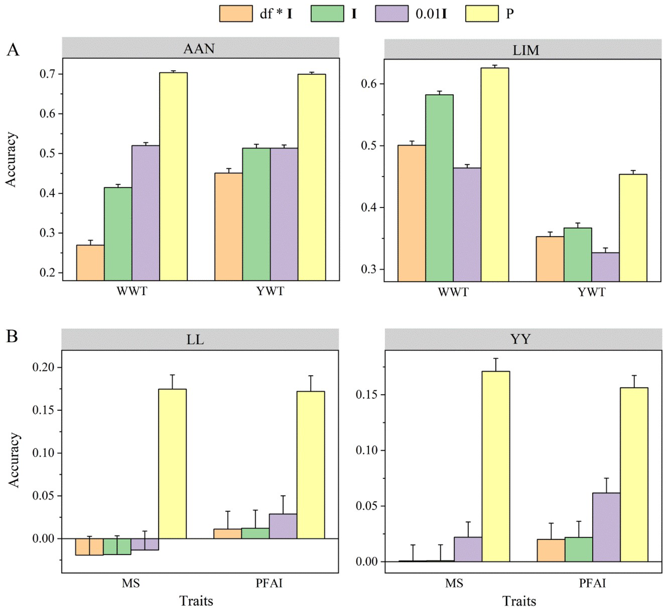
Figure 2.
Prediction accuracy of the model using different degrees of freedom (df) in IW prior to random effects in mbBayesAB. The dataset comprised beef cattle data (A) from two breeds, Limousin (LIM) and Angus (AAN), and pig data (B) from two breeds, Large White (YY) and Landrace (LL). The analyzed traits included marbling score (MS), fat area ratio in the image (PFAI), yearling weight (YWT), and weening weight (WWT). Prediction accuracy was derived from a five-fold CV of 10 replicates. The scale parameter in IW prior was estimated from the phenotype variance (details in the Section 2). The “p” in the legend represents the number of breeds.
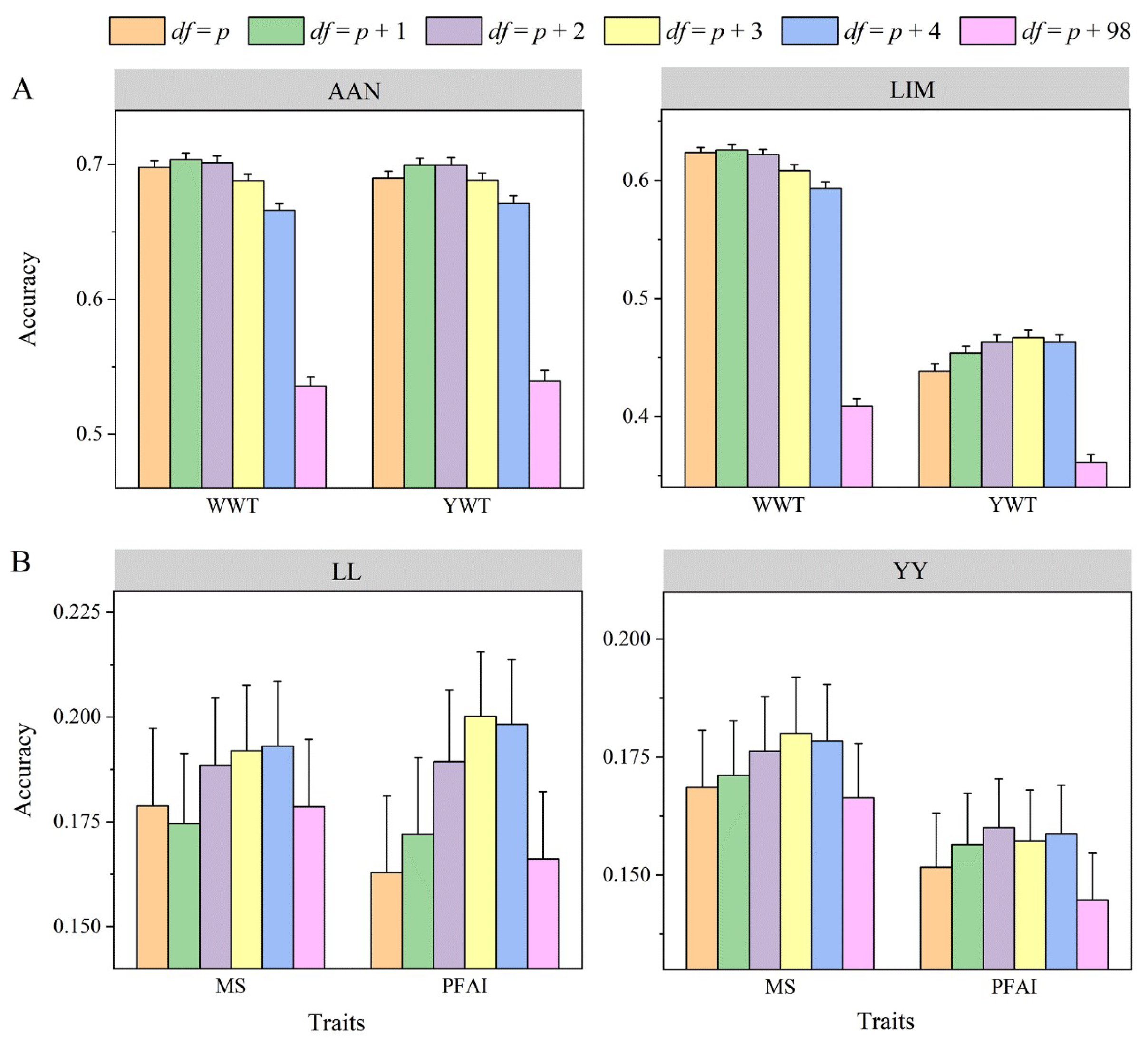
Figure 3.
Prediction accuracy of mbBayesAB model when partitioning the genome using different numbers of adjacent SNPs. The dataset comprised beef cattle data (A) from two breeds, Limousin (LIM) and Angus (AAN), and pig data (B) from two breeds, Large White (YY) and Landrace (LL). The analyzed traits included marbling score (MS), fat area ratio in image (PFAI), yearling weight (YWT), and weening weight (WWT). Prediction accuracy was derived from five-fold CV of 10 replicates. The degree of freedom was set to p + 3 and the scale parameter in IW prior was estimated based on phenotype variance (details in the Section 2).
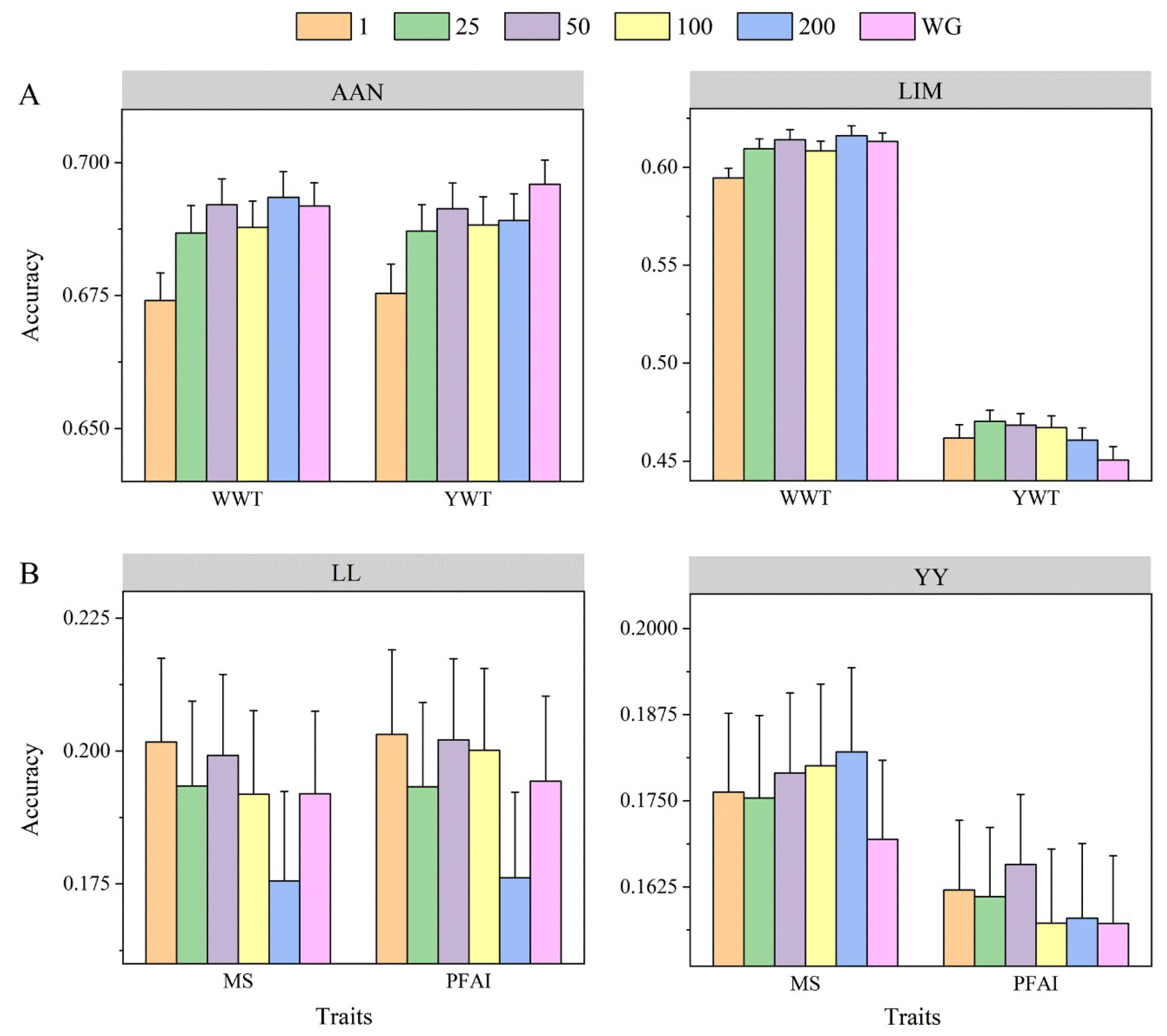
Figure 4.
Prediction accuracies of different models in real data analysis. The dataset comprised beef cattle data (A) from two breeds, Limousin (LIM) and Angus (AAN), and pig data (B) from two breeds, Large White (YY) and Landrace (LL). The analyzed traits included marbling score (MS), fat area ratio in the image (PFAI), yearling weight (YWT), and weening weight (WWT). The reference population in the w-GBLUP only contains individuals of the same breed as the validation, and the references for the other three models contain individuals of two breeds. For u-GBLUP and mbBayesAB, the same traits of different breeds were regarded as genetically related different traits, and in b-GBLUP, two breeds were blended, and then single-trait GBLUP was used for prediction. Predictive accuracy was derived from five-fold CV of 10 replicates. The degree of freedom was set to p + 3 and the scale parameter in IW prior was estimated based on phenotype variance (details in the Section 2).


Table 1.
Estimates of heritability for analyzed traits across different breeds.
| Species | Traits 1 | Breed 2 | Records | Va 3 | Ve 4 | h2 (SE) 5 |
|---|---|---|---|---|---|---|
| Pig | PFAI | YY | 641 | 0.31 | 1.30 | 0.19(0.07) |
| LL | 228 | 0.67 | 1.35 | 0.33(0.16) | ||
| MS | YY | 641 | 0.05 | 0.18 | 0.22(0.07) | |
| LL | 228 | 0.09 | 0.20 | 0.31(0.16) | ||
| Beef cattle | YWT | LIM | 1528 | 1601.40 | 1497.88 | 0.52(0.05) |
| AAN | 796 | 1116.65 | 340.43 | 0.77(0.04) | ||
| WWT | LIM | 1897 | 3133.74 | 994.59 | 0.76(0.03) | |
| AAN | 797 | 347.75 | 94.44 | 0.79(0.04) |
1 WWT, weening weight; YWT, yearling weight; MS, marbling score; PFAI, fat area ratio in image; 2 LIM, Limousin; AAN, Angus; YY, Large White; LL, Landrace; 3 additive genetic variances; 4 residual variances; 5 heritability and estimated standard error.
Table 2.
Prediction accuracy when specifying different priors for the (co)variance matrix of random effects in the mbBayesAB model.
Table 2.
Prediction accuracy when specifying different priors for the (co)variance matrix of random effects in the mbBayesAB model.
| Species | Breed 1 | Traits 2 | Prior 3 | Genetic Correlation 4 | Accuracy 5 |
|---|---|---|---|---|---|
| Beef cattle | AAN | WWT | IW | 0.065 ± 0.005 | 0.704 ± 0.005 |
| HIW-WI | 0.053 ± 0.006 | 0.699 ± 0.005 | |||
| HIW-IG | 0.050 ± 0.005 | 0.698 ± 0.005 | |||
| YWT | IW | 0.050 ± 0.005 | 0.700 ± 0.005 | ||
| HIW-WI | 0.039 ± 0.006 | 0.698 ± 0.005 | |||
| HIW-IG | 0.051 ± 0.005 | 0.690 ± 0.005 | |||
| LIM | WWT | IW | 0.065 ± 0.005 | 0.626 ± 0.005 | |
| HIW-WI | 0.053 ± 0.006 | 0.624 ± 0.005 | |||
| HIW-IG | 0.050 ± 0.005 | 0.623 ± 0.004 | |||
| YWT | IW | 0.050 ± 0.005 | 0.454 ± 0.006 | ||
| HIW-WI | 0.039 ± 0.006 | 0.452 ± 0.006 | |||
| HIW-IG | 0.051 ± 0.005 | 0.438 ± 0.006 | |||
| Pig | LL | MS | IW | −0.071 ± 0.007 | 0.175 ± 0.017 |
| HIW-WI | −0.035 ± 0.008 | 0.186 ± 0.018 | |||
| HIW-IG | −0.038 ± 0.007 | 0.179 ± 0.019 | |||
| PFAI | IW | −0.081 ± 0.007 | 0.172 ± 0.018 | ||
| HIW-WI | −0.057 ± 0.007 | 0.160 ± 0.019 | |||
| HIW-IG | −0.069 ± 0.006 | 0.163 ± 0.018 | |||
| YY | MS | IW | −0.071 ± 0.007 | 0.171 ± 0.012 | |
| HIW-WI | −0.035 ± 0.008 | 0.172 ± 0.012 | |||
| HIW-IG | −0.038 ± 0.007 | 0.169 ± 0.012 | |||
| PFAI | IW | −0.081 ± 0.007 | 0.156 ± 0.011 | ||
| HIW-WI | −0.057 ± 0.007 | 0.155 ± 0.011 | |||
| HIW-IG | −0.069 ± 0.006 | 0.152 ± 0.011 |
1 LIM, Limousin; AAN, Angus; YY, Large White; LL, Landrace; 2 WWT, weening weight; YWT, yearling weight; MS, marbling score; PFAI, fat area ratio in image; 3 priors for the (co)variance matrix of random effect. IW represents the (co)variance matrix assigned to an IW prior assuming that the scale matrix is known, IW-WI represents an IW prior for which the scale matrix follows the Wishart distribution, IW-IG represents an IW prior for which the scale matrix follows the inverse gamma distribution (details in the Section 2); 4 an estimate of the genetic correlation (standard errors) between breeds across the entire genomic region, calculated from the correlation of marker effects between two breeds in the pig or beef cattle population; 5 prediction accuracy (standard errors) was derived from five-fold CV of 10 replicates.
Disclaimer/Publisher’s Note: The statements, opinions and data contained in all publications are solely those of the individual author(s) and contributor(s) and not of MDPI and/or the editor(s). MDPI and/or the editor(s) disclaim responsibility for any injury to people or property resulting from any ideas, methods, instructions or products referred to in the content. |
© 2024 by the authors. Licensee MDPI, Basel, Switzerland. This article is an open access article distributed under the terms and conditions of the Creative Commons Attribution (CC BY) license (https://creativecommons.org/licenses/by/4.0/).
Share and Cite
MDPI and ACS Style
Li, W.; Zhang, M.; Du, H.; Wu, J.; Zhou, L.; Liu, J. Multi-Trait Bayesian Models Enhance the Accuracy of Genomic Prediction in Multi-Breed Reference Populations. Agriculture 2024, 14, 626. https://doi.org/10.3390/agriculture14040626
AMA Style
Li W, Zhang M, Du H, Wu J, Zhou L, Liu J. Multi-Trait Bayesian Models Enhance the Accuracy of Genomic Prediction in Multi-Breed Reference Populations. Agriculture. 2024; 14(4):626. https://doi.org/10.3390/agriculture14040626
Chicago/Turabian StyleLi, Weining, Meilin Zhang, Heng Du, Jianliang Wu, Lei Zhou, and Jianfeng Liu. 2024. "Multi-Trait Bayesian Models Enhance the Accuracy of Genomic Prediction in Multi-Breed Reference Populations" Agriculture 14, no. 4: 626. https://doi.org/10.3390/agriculture14040626
Note that from the first issue of 2016, this journal uses article numbers instead of page numbers. See further details here.