Article

An Accurate Approach for Predicting Soil Quality Based on Machine Learning in Drylands

by
Radwa A. El Behairy
1,
Hasnaa M. El Arwash
2,
Ahmed A. El Baroudy
1,
Mahmoud M. Ibrahim
1,
Elsayed Said Mohamed
3,4,
Nazih Y. Rebouh
4 and
Mohamed S. Shokr
1,*
1
Soil and Water Department, Faculty of Agriculture, Tanta University, Tanta 31527, Egypt
2
Mechatronics Engineering Department, Alexandria Higher Institute of Engineering & Technology (AIET), Alexandria 21311, Egypt
3
National Authority for Remote Sensing and Space Sciences, Cairo 1564, Egypt
4
Department of Environmental Management, Institute of Environmental Engineering (RUDN University), Moscow 117198, Russia
*
Author to whom correspondence should be addressed.
Agriculture 2024, 14(4), 627; https://doi.org/10.3390/agriculture14040627
Submission received: 29 February 2024 / Revised: 12 April 2024 / Accepted: 16 April 2024 / Published: 18 April 2024
(This article belongs to the Special Issue Applications of Data Analysis in Agriculture—2nd Edition)

Abstract

:
Nowadays, machine learning (ML) is a useful technology due to its high accuracy in constructing non-linear models and algorithms that can adapt to the complexity and diversity of data. Thus, the current work aimed to predict the soil quality index (SQI) from extensive soil data, achieving high accuracy with the artificial neural networks (ANN) model. However, the efficiency of ANN depends on the accuracy of the data that is prepared for training. For this purpose, MATLAB programming language was used to enable the calculation, classification, and compilation of the results into databases within a few minutes. The proposed MATLAB program was highly efficient, accurate, and quick in calculating soil big data for training the machine compared with traditional methods. The database contains 306 vector sets, 80% of them are used for training and the remaining 20% are reserved for testing. The optimal model obtained comprises one hidden layer with 250 neurons and one output layer with a sigmoid function. The ANN achieved a high coefficient of determination (R2) values for SQI estimation, with around 0.97 and 0.98 for training and testing, respectively. The results indicate that 36.93% of the total soil samples belonged to the very high quality class (C1). In contrast, the high quality (C2), moderate quality (C3), low quality (C4), and very low quality (C5) classes accounted for 10.46%, 31.37%, 20.92%, and 0.33% of the samples, respectively. The high contents of CaCO3, pH, sodium saturation, salinity, and clay content were identified as limiting factors in certain areas. The results of this study indicated high accuracy of soil quality assessment using physical, chemical, and fertility soil features in regression analysis with ANN. This method, which is suitable for arid zones, enhances agricultural productivity and decision-making by identifying critical soil quality categories and constraints.

1. Introduction

It is expected that global food demand will increase by 70% by 2050 because of the rapid growth of global population which may exceed 9 billion, and consequently lead to human food insecurity [1,2]. Developing countries such as Egypt face food security challenges due to the growth of population and the shortage of agricultural resources [3,4]. Soil is one of the critical resources that can help fill the gap in food demand and ensure food security [3]. However, in recent decades, rapid growth in industry and agriculture, as well as degradation and degrading the earth’s environment in various ways, have posed a significant challenge in promoting environmental sustainability and improving agricultural productivity [5,6,7].
Soil quality is very important to focus on for the sustainable use of agricultural lands [8,9]. Soil quality assessment can improve soil fertility, conserve soil, improve soil environmental integrity, protect human health, and ensure long-term soil productivity [5,10]. Therefore, to protect and improve the quality of farmlands, it is necessary to assess and search for soil quality, also improve agricultural productivity, and assist in food planning for the ever-growing global population. However, comprehensive soil quality studies in drylands have received little attention [10]. There are many complex methods to create a soil quality index. This process includes selecting indicators, scoring, and then combining them into a single index [11]. Soil physicochemical properties are indicators of soil quality, reflecting ecosystem stability. Therefore, selecting appropriate evaluation methods is critical to accurately assessing soil quality [12,13].
Artificial intelligence (AI) and machine learning (ML) techniques are successfully being applied in agriculture. ML techniques use computer algorithms and sample data to create a model for decision-making without explicit programming [14]. ML algorithms utilize past experiments to establish successful relationships for data inputs, rebuild the knowledge schema, and process them for future prediction [15,16]. They are used in agriculture [17,18,19], especially in determining soil quality [20,21,22], to enhance efficiency, reduce production costs, and minimize environmental impact [23,24]. Machine learning methods can be supervised [25], unsupervised [26], or reinforcement learning [27]. Artificial neural networks (ANN) are an example of an ML method under supervised learning and can be used to optimize agricultural management [16,22,28]. Supervised learning builds a model to predict the output from input data. It provides better accuracy for regression and classification problems [14].
Artificial neural networks (ANN) have been used by several researchers to predict soil attributes based on different variables [21,29,30]. ANN have proven to be successful in solving complex problems in various agricultural research fields [31,32], especially when the fundamental correlation is unclear. They can recognize and learn types of correlation between independent variables and dependent target variables. Then, they can estimate the dependent variables using recent independent variable datasets [33]. ANN are also error-tolerant, adaptive to work with incomplete data, and to make decisions even in uncertain situations [21]. The main drawback of the classical method is that it requires a linear mathematical operation that cannot satisfy the objective function in nonlinear conditions [34]. Artificial neural networks (ANN) are comprised of three main types of neurons: the input layer, the hidden layer, and the output layer [35]. These layers work in parallel, mimicking the structure and function of the human brain. The parallel information transmission between neurons is represented by these layers. Because of this arrangement, ANN can compute faster than a sequential system [35] as each data set in ANN has different activation functions, neurons, and layers that can have different results. Therefore, artificial neural networks are currently considered the most preferred method to estimate soil quality in farmland [22].
Big data refers to the practice of gathering and scrutinizing large quantities of data sets to uncover valuable and useful insights and patterns. Big data is utilized in various advanced analytic techniques such as machine learning, deep learning, and predictive modeling to help solve workplace problems and make more informed decisions [16,36]. Additionally, agricultural big data is a collection of technologies that can help farmers face the challenges of the new era of data. When combined with machine learning, it enables farmers to use data to address various issues such as decision making, water and soil management, and crop and livestock management [16].
Programming languages are classified into two generations: third-generation languages such as C, C++, Python, and Java and fourth-generation languages such as Matlab, which stands for Matrix Laboratory. Third-generation languages are general-purpose and provide granular control to create fast applications. Fourth-generation languages are designed for scientific and technical computing and are ideal for data-driven fields [37]. Matlab has a programming capability via written codes that allows users to create functions for intended activities, making it fast and ideal for calculations [38]. It is used for soil quality assessment because of its ability to perform high-accuracy calculations, store results digitally, and modify data easily with efficient, easy-to-use window-based software [39,40].
The aims of this work were as follows:
  • To propose an accurate approach for assessment soil quality, used in Egypt, using 16 features and their scores depending on Matlab codes. The codes are available for calculating the SQI for other regions, just by changing the dataset and updating the scoring criteria. A MATLAB program was developed to calculate soil quality, classify it, and compile the results into useful databases. This will contribute to big data analysis in a systematic, reliable, accurate, and timely manner compared to traditional methods.
  • To use the artificial neural network model for SQI prediction with 306 datasets of soil samples based on one hidden layer with a number of neurons and one output layer. To improve the performance and generalization ability of the model, hyperparameter tuning and K-fold cross-validation were carried out in this paper. Then, the optimal number of neurons was determined to obtain the most effective and accurate predictive model in this study evaluating the metrics (MSE and R).

2. Materials and Methods

In this section, the sequence of work is demonstrated as shown in Figure 1 and will be explained in detail in the following subsections.

2.1. Experimental Zones and Soil Sampling

Three unmanaged areas were selected in many different governorates in Egypt (Figure S1). The first zone is situated on the northwest coast of the western region of Matrouh governorate [41]. The Wadi Al-Halaazin area is located at 26°49′06″ to 26°58′00″ E longitudes and 31°13′00″ to 31°26′03″ N latitudes with a total area of 21,369.74 hectares. Information on spectral satellite (sentinel 2 acquired in April 2020) was used in this zone.
The second zone is situated in the northern part of the Nile Delta, in Kafr El Sheikh governorate [42]. The zone is located between longitudes 31°00″ and 31°15″ East, and latitudes 31°00′ and 31°37′ North, covering a total area of 156 Kha. It is bordered to the north by the Mediterranean Sea; to the south by Gharbia Governorate; to the east by Dakahlia Governorate, and to the west by Sidi Salem and Kafr El-Sheikh district. Digital image processing for Thematic Mapper TM image (1983) and Enhanced Thematic Mapper ETM+ (2003) images was performed using ENVI 4.3 software in this zone.
The third zone, in the middle of the first and the second zones, is located northwest of the Nile Delta [43]. This zone is located between the coordinates 30°15′0″ and 30°40′0″ E and 31°7′15″ and 31°30′45″ N, with a total area of 79.700 hectares. In this zone, a sentinel-2 image acquired in August 2020 under clear-sky conditions was utilized. These zones were selected to assess soil quality for better and more accurate assessment on a large scale.
Three datasets for these zones were created having entirely different properties. The first dataset consisted of 118 soil samples, called here as the first zone soil dataset. Also, the second dataset consisted of 112 soil samples, called the second zone soil dataset, while the third zone soil dataset consisted of 76 soil samples. Soil samples for these datasets were collected in various locations having a very different texture and physio-chemical content variation. The global positioning system (GPS) tagged the soil samples with their location, and they were dug up and described according to [44,45]. In total, we collected 306 soil samples that covered various recognized soil layers. After air-drying the soil samples and sieving the fine earth (<2 mm) particles with a 2 mm sieve, we conducted a complete chemical analysis on them. These soil sample analyses were carried out based on [46] by an accredited soil, water, and plant laboratory in compliance with the requirements of [47] at the Faculty of Agriculture, Tanta University.
The soil quality index (SQI) is comprised of three primary groups, each with its own set of indicators. These groups are as follows:
(i)
Chemical indicators: This group includes indicators such as cation exchange capacity (CEC), the percentage of calcium carbonate (CaCO3), the percentage of exchangeable sodium (ESP), gypsum (CaSO4), electrical conductivity (EC), and soil reaction (pH).
(ii)
Physical indicators: This group includes soil depth (SD), soil slope (SS), bulk density (BD), soil texture (ST), water holding capacity (WHC), and hydraulic conductivity (HC).
(iii)
Fertility indicators: This group includes soil organic matter (SOM), available nitrogen (AvN), available phosphorus (AvP), and available potassium (AvK).
Soil quality features are defined as soil processes and characteristics sensitive to fluctuation caused by both natural and human-induced indicators. As a result, soil quality metrics can be classified as dynamic or static [21]. Furthermore, soil quality studies are primarily concerned with dynamic soil parameters, which may be significantly influenced by soil management [48]. Therefore, native indicators such as soil texture, particle size distribution, and mineral content type, are difficult to modify in a short period of time, whereas dynamic indicators, such as plant nutrient element concentration, reveal soil circumstances caused by current soil management or agrotechnology [21]. Thus, the rising heavy metal concentration in Egypt’s soils influences negatively the quality of soil and water, which is also linked to soil fertility and food security [49,50,51,52,53]. Soil salinity, soil reaction (pH), and proportion of soil calcium carbonate are among the parameters that influence soil physicochemical properties [31]. Thus, the most studied aspects to assess soil quality are nutritional elements, soil organic matter, and hydraulic properties [54]. Soil quality can be measured using physical indicators such as bulk density, root depth, and soil texture, as well as chemical indicators such as cation exchange capacity (CEC), soil salinity, and pH. There are significant relationships among these parameters and soil quality [55,56]. As a result, texture is a highly effective attribute in terms of water and nutrient retention, aeration, and root growth, as it contributes significantly to soil quality [22,57,58]. In addition, hydraulic conductivity (HC) is an indicator of the movement of water and the pore structure in soil [59]. In general, soil organic matter (SOM) plays a vital role in enhancing the physical and chemical properties of soil [60,61]; that is, the soil’s water holding capacity and nitrogen cycle are directly affected by any increase in the content of SOM in the soil [62]. On the contrary, depletion of SOM can cause a decline in the cation exchange capacity, the aggregate stability, and the yield productivity. Hence, it can negatively impact soil quality [63,64]. In order to improve the quality of soil and water, it is important to use accurate measurements and effective procedures [65].

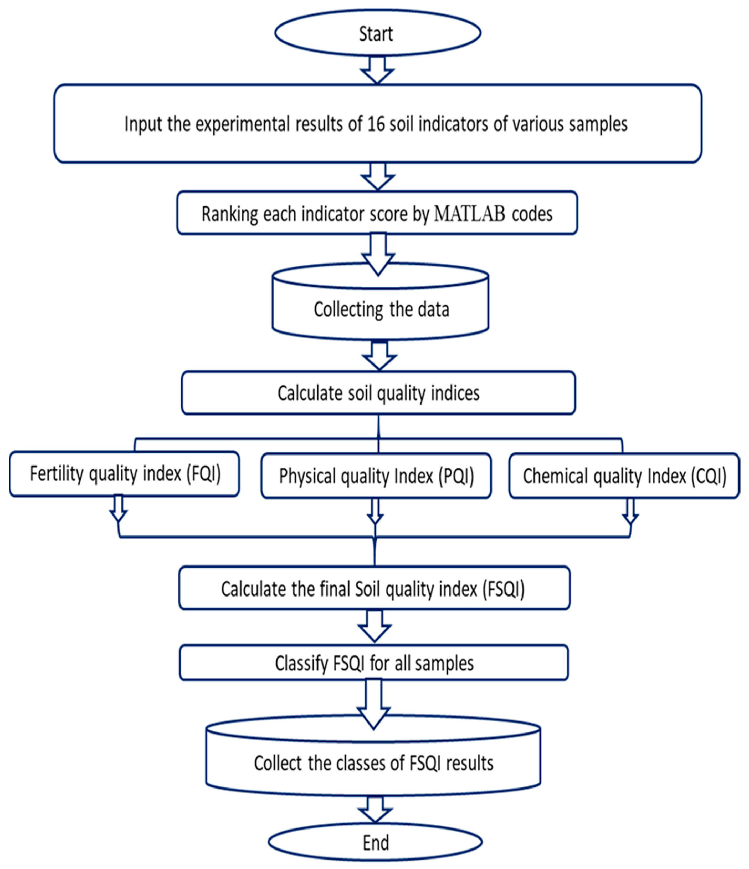
2.2. Soil Quality Index Database Using MATLAB Codes

The process of soil quality assessment using the Matlab program can be summarized in the flowchart shown in Figure 2 and is explained in detail in the following steps:
  • First, the experimental results of 16 soil indicators, that is, SOM, AvK, AvP, AvN, HC, WHC, BD, ST, SS, SD, CEC, CaSO4, CaCO3, ESP, pH, and EC for the various samples used in this study were added as inputs.
  • Next, each indicator score was ranked in MATLAB environment according to Tables S1–S3.
  • A special database was built to collect each indicator score for various samples under study.
  • The soil quality indices were calculated as described in detail in Section 2.3.
  • In this step, the final soil quality index (FSQI) was calculated as described in Section 2.3.
  • The values of FSQI were classified for all samples.
  • Finally, a new database, with the classes of FSQI results for each investigated sample was created.

2.3. Soil Quality Model

The following text discusses the mathematical model used to calculate the index of soil quality (SQI) in detail. SQI is calculated using the geometric mean algorithm (GMA) methodology, which involves finding the nth root of a sequence of values, as shown in Equation (1). GMA has been widely used to assess soil quality and crop suitability, as presented in most recent studies [3,51,66,67,68,69,70].
I n d e x x = S 1 × S 2 × S 3 × × S n n
where
  • x: the quality index
  • S: the parameter’s score
  • n: the parameter’s number
In this study, the researchers utilized a soil quality index that consists of three indices, namely, chemical (CQI), physical (PQI), and fertility (FQI), to evaluate soil quality. The chemical quality index can be calculated using Equation (2) as follows:
C Q I = E C × p H × E S P × C a C O 3 × C a S O 4 × C E C 6
where
  • CQI: chemical quality index
  • EC: electric conductivity
  • pH: soil reaction
  • ESP: exchangeable sodium percentage in soil
  • CaCO3: soil calcium carbonate
  • CaSO4: percentage of gypsum
  • CEC: cation exchange capacity
To calculate the index of physical quality, Equation (3) is used as follows:
P Q I = H C × W H C × B D × S T × S S × S D 6
where
  • PQI: physical quality index
  • HC: hydraulic conductivity
  • WHC: water holding capacity
  • BD: bulk density
  • ST: soil texture
  • SS: soil slope
  • SD: soil depth
Equation (4) is used to define the fertility quality index.
F Q I = S O M × A v K × A v P × A v N 4
where
  • FQI: fertility quality index
  • SOM: soil organic matter
  • AvK: available potassium
  • AvP: available phosphorus
  • AvN: available nitrogen
Soil chemical, physical, and fertility quality indices are integrated together to classify the final soil quality index (FSQI) using the mathematical equation shown in Equation (5):
F S Q I = C Q I × P Q I × F Q I 3
where
  • FSQI: the index of final soil quality
  • CQI: the index of chemical quality
  • PQI: the index of physical quality
  • FQI: the index of fertility quality
The parameters are scored on a scale of 0.2 to 1, where 0.2 is the worst condition and 1 is the best condition. Based on several sources [44,71,72,73,74,75,76], the scores for each parameter are presented in Tables S1–S3. Figure 3 shows part of the proposed program code using MATLAB to calculate the EC score.
The final soil quality index (FSQI) values are divided into five classes (Table S4). These classes are very high quality (C1), high quality (C2), moderate quality (C3), low quality (C4), and very low quality (C5). The width of each class is determined by dividing the range of values for the index by the total number of classes (which is 5). The top limits of each class are then determined by sequentially adding the obtained values to the index’s lowest values. This approach was used in various studies by [51,67,68]. Figure 4 depicts part of the proposed program code using MATLAB to calculate classes of FSQI.

2.4. Soil Quality Index (SQI) Assessment in Big Data

The calculations were performed in three different scenarios, as follows:
Scenario 1: 150 different samples.
To hold soil features, 150 soil samples are used, and a matrix of size (m × n) is created in this study. Similarly, a soil indices matrix of size (m × n) is created to classify the input soils and facilitate calculations. The size of the soil indices matrix is 16 rows by 150 columns, where m represents soil indices and n represents different soil samples. Soil quality using 16 soil indicators is evaluated, and a program to determine the class of final soil quality index for each sample is also run.
Scenario 2: 306 different samples.
Scenario 3: 700 different samples.
For the three scenarios mentioned above, the proposed program consists of four major steps:
  • Data analytics: The best way to organize big data analysis is to put it in the form of matrices so that we can keep track of the data.
  • Data classification: Structured rules are used in big data classification using MATLAB.
  • Comparison with traditional method calculations for quality (effectiveness and accuracy) and time consumption.
  • Finally, validating the proposed program.

2.5. Soil Quality Prediction Using ANN

In order to enable the system to learn from high-quality data on its own, ANN algorithms are created by combining a parameterized module. To ensure the system is reliable, the primary task is to estimate the soil experimental analysis and define the soil quality index for hundreds of soil samples. In this study, the total dataset of 306 samples is divided as follows:
-
A training dataset of 245 data points is required to build the model. The obtained data is randomly divided into training sets of 70% and testing sets of 30%.
-
A test dataset of 61 data points is required to estimate the model’s performance.
In order to determine the most suitable number of neurons for the hidden layers in this application, the training process is repeated several times with different numbers of neurons: 50, 100, 150, 200, 250, and 260. The results of training and testing are then compared and analyzed.
Figure 5 illustrates the computational flow diagram of the established hybrid ANN model, which involves cross-validation using k-fold and BOA.
As shown in Figure 5, the ANN-based scheme can be used to forecast SQI. The first ANN training structure, proposed in this study, is to determine the content of experimental soil analysis. Sixteen soil parameters derived from 306 soil samples are used as input signals. Feed-forward neural network takes these sampled values at each examined point as input signals without any pre-processing. The neural networks used to assess soil quality consist of three layers: input layer, one hidden layer, and output layer. The input layer contains 16 neurons representing 16 experimental soil tests. The network’s capacity to generalize the detection process dictates the number of neurons in the hidden layers. Many trials are made to determine which hidden layer of neurons is the best fit for the network’s soil quality. The sigmoid function is the most suitable activation function for hidden layers.
Mean square error (MSE) and the coefficient of determination (R2) are used to validate the performance measurement of the ANN model and are calculated, as shown in Equations (6) and (7) [21,77]. These equations represent the network’s output value of 0.0001 and show how to adjust the network’s weight and bias based on the mean square error (MSE). The value of the target weight is predicted by the ANN algorithm using the smallest estimate of the MSE being close to zero, which measures its effectiveness [78].
M S E = 1 n i = 1 n Y i y ^ i 2
R 2 = 1 i = 1 n Y i y ^ i 2 i = 1 n Y i y i ¯ 2
where
  • n: the number of experimental data sets
  • y ^ i : the actual soil quality value
  • Y i : the predicted soil quality value
  • y i ¯ : the mean of the target output data
The activation function is crucial in a neural network as it enables the representation of the actual relationship between input and output. Without it, the neural network produces a simple linear function, limiting its complexity to that of a basic first-degree polynomial function. A neural network without an activation function operates as a linear regression model, which is usually limited in performance and power, making it unsuitable for learning and identifying complex mappings from data. Therefore, an activation function is critical for a neural network to model complex data types like images, videos, audio, speech, text, etc. [79]. The relationship between the input, hidden, and output layers can be expressed using Equation (8), which shows the correlation between these levels:
y i = f i = 1 N w i x i + b
where
  • N: the number of input parameters
  • wi: the weighted average of input parameters
  • xi: the input parameters
  • b: the bias function
The bias function ‘b’ is used to optimize input data in an ANN model. During the training process, the initial weight ‘w’ is gradually corrected, and the estimated results are compared to the targets. Any errors are then back-propagated. The data are trained using the back-propagation (BP) technique [80], specifically the scaled conjugate gradient (trainscg) algorithm. These procedures are repeated until a specific value of root mean square error (RMSE) is achieved, through updating the values of both ‘w’ and ‘b’.
It is unclear what sample size is appropriate when using artificial neural networks (ANN) in a particular context. However, it is commonly recommended that the sample size be at least 10 to 100 times the number of features [81,82]. This study used 16 different features (such as SOM, AvK, AvP, AvN, HC, WHC, BD, ST, SS, SD, CEC, CaSO4, CaCO3, ESP, pH, EC) to create the model. Therefore, the minimum number of samples required is 160. The total number of samples used in this study was 306, which is more than the minimum required sample size of 160. The optimal structure of the ANN network is influenced by various hyperparameters including the number of hidden layers, hidden neurons, and learning rate. All hyperparameter tuning was conducted using the k-fold cross-validation and Bayesian optimization algorithm (BOA) approaches [83,84,85,86,87,88].
The data set is split into k subsets. One subset is selected as the test data, while the rest are used for training. This process is repeated k times to ensure each subset is tested only once.
The Bayesian optimization algorithm (BOA) is designed to select the best hyperparameters that can minimize validation errors. The Bayesian backpropagation algorithm is used to train the system. In the training phase, the proposed MATLAB program is utilized to train the ANN system using the soil quality index. BOA optimization can be expressed in Equation (9), which helps in minimizing validation error, given a hyperparameter space X and an objective function f:
x * = arg min xϵX f ( x )
where
  • x * : is the set of hyperparameters that produce the minimum target score
  • x: is any value in the space X
The term ‘optimization’ commonly refers to the process of finding the maximum or minimum value of an objective function. In most cases, this function is unknown and lacks an analytical expression. Optimization is the global optimization of a black-box function with an unknown equation and derivatives [89,90]. This method performs better than random, manual, or grid search algorithms [91]. It involves using a surrogate probability model based on the Bayes theorem [92]. This model selects the values for the next iteration based on the results of the previous iterations, which results in more effective optimization than arbitrary selection. The experiment results can be summed up as follows:
p w D = p w D p ( w ) p ( D )
where
  • p w : is the prior probability
  • p D : is the evidence, p D w refers to the probability
  • p w D : is the posterior probability
This method involves identifying the optimal point to evaluate by means of using the acquisition function, which is based on the surrogate model. The Gaussian process (GP) is capable of simulating p w D . The mean value function (μ) and the covariance function (K) of the model are expressed as follows [83,84,85,86,87,88]:
f x ~ G P ( μ , K )
Generally, BOA can be described as a process that consists of the following steps:
  • Step one: Create an objective function that minimizes validation errors.
  • Step two: Develop a surrogate probability model for the objective function.
  • Step three: Determine the optimal hyperparameters for the surrogate probability model.
  • Step four: Apply these hyperparameters to the actual objective function.
  • Step five: Combine the new findings to improve the surrogate model.
  • Step six: Repeat steps three to five until the maximum number of iterations is reached.

3. Results and Discussion

3.1. Soil Physicochemical Features

Descriptive statistics of soil properties are presented in Table 1. EC values in soil samples varied between 0.55 and 129.70 dSm−1, with an average value of 5.46 ± 10.91 dSm−1. The results are consistent with the environmental conditions of drylands, which have high rates of evaporation and low precipitation that results in most salinized soils [3,93]. High soil salinity in certain areas can be attributed to the high salinity of the water table and the effects of lake water and seawater [51,94,95]. Various soil management options have been proposed to decrease soil salinity, such as using low-salinity water to enhance the leaching of salts from the soil root zone [49,96]. The rate of plant growth under salt stress varies significantly among different plant species [97,98]. The soil salinity relations with ESP and CaCO3 reveal that soil salinity is primarily due to Na+, Ca2+, CO32−, and HCO3 [99]. The range of ESP values is 1.45% to 35.93%, with an average value of 9.29 ± 7.50%. A high sodium percentage can negatively impact soil properties such as soil structure and hydrology, leading to reduced crop productivity [3]. The value of CaCO3 in soil samples varied from 0.21 to 34.42%. The highest values of CaCO3 are due to shell fragments, which can lead to the formation of solid layers impermeable to crops and water, as well as the fixation of P fertilizer [3,100]. CaCO3 has a positive effect on soil quality by enhancing WHC and reducing HC [6]. Previous studies demonstrated that adding gypsum can lower the high soil sodium saturation content [73,101], because of its ability to absorb calcium instead of sodium in soil particles, which causes aggregation improvement and pH decline [101,102]. CaSO4 ranged from 0.07% to 9.68% with an average of 1.21%. The soil reaction (pH) was maximum 9.21, and minimum 7.46. High pH values may have resulted from low macro-nutrients levels, which cause low vegetation [103].
The available N ranged from 3.10 to 98.91 mgKg−1. Moreover, minimum, and maximum values of available phosphorus ranged from 2.09 to 38.45 mgKg−1, while available potassium varied between 7.70 and 719.10 mgKg−1. The content of soil organic matter ranged from 0.01% to 2.96%, with an average of 0.63%. The results of CEC ranged from 0.95 to 58.40 cmolcKg−1. The low values of CEC are primarily caused by inadequate amounts of clay and organic matter since there is a substantial positive correlation between CEC, clay content, and organic matter [104].
Reduced levels of available macro-nutrient (N, P, K), SOM%, and CEC adversely impact soil quality. Additionally, physical characteristics such as shallow depth and coarse texture disrupt the arrangement of particles and pores in the soil, thereby impeding root growth and plant emergence velocity. Moreover, these factors also affect water infiltration during agricultural practices [59]. The soils were flat to sloping with a slope range of 0.10 to 8%. The depth of soils (SD) varied from 30 to 150 cm. There are differences in soil texture between sand, loamy sand, sandy loam, sandy clay loam, clay, silty clay, silty clay loam, silty loam, loam, and clay loam. Fine earth has a significant effect on soil quality because soils originating from coarse sands are deep with poor physical properties such as high density, rapid infiltration rate, and low water retention [105]. The bulk density (BD) values of the soils varied between 1.16 gcm−3 and 1.68 gcm−3 depending on the organic matter content and especially the amount of sand and clay. Soil water holding capacity (WHC) and hydraulic conductivity (HC) ranged from 3.01 to 53.04% and from 0.29 to 33.42 cmhr−1, respectively. Increasing the medium (silt) and fine (clay) particles might improve these conditions, as these fractions block soil macro-pores, by decreasing BD and HC, and improving WHC [106].
According to the results obtained, the BD and SD values are left skewed (−) as compared to the normal distribution. On the other hand, the values of other features exhibit a right skewness (+) distribution. The feature with the highest skewness coefficient and the farthest distribution from the normal was determined as EC. The data show that the curves of most soil properties have low kurtosis and tend to have light tails or lack of outliers relative to a normal distribution. The coefficient of variation (CV) defines the degree of variability where CV values below 20, 20–50, and above 50% indicate low, moderate, and large variability [107]. Hence, all the studied soil properties had large variabilities, meaning that there is a high variability of soil parameters and soil quality (SQ) within soil samples in the study zones, except for the pH and BD (low variability), and the soil depth (SD) (moderate variability).

3.2. Soil Quality Index Using MATLAB Proposed Program

3.2.1. Scenario 1

Figure 6 shows a comparison between the soil quality index calculations using Matlab and traditional methods. It can be observed that the traditional methods have significant differences in some soil samples for the soil quality classes, which validate the accuracy of the proposed program.

3.2.2. Scenario 2

In this scenario, we considered a total of 306 soil samples. This study involved assessing the quality of the soil using 16 different indicators. As a result, the soil features matrix has 16 rows and 306 columns. The program was modified and executed to perform the soil quality calculation. Figure 7 illustrates noticeable variations in soil quality classes with traditional methods, which confirms the accuracy of the proposed program.

3.2.3. Scenario 3

For this study, 700 soil samples were analyzed. The soil features matrix has 16 rows and 700 columns, with each column representing a different soil sample. To determine the class of final soil quality index, the program was modified and run accordingly. Figure 8 depicts a plot of the obtained results from traditional methods and the proposed program.

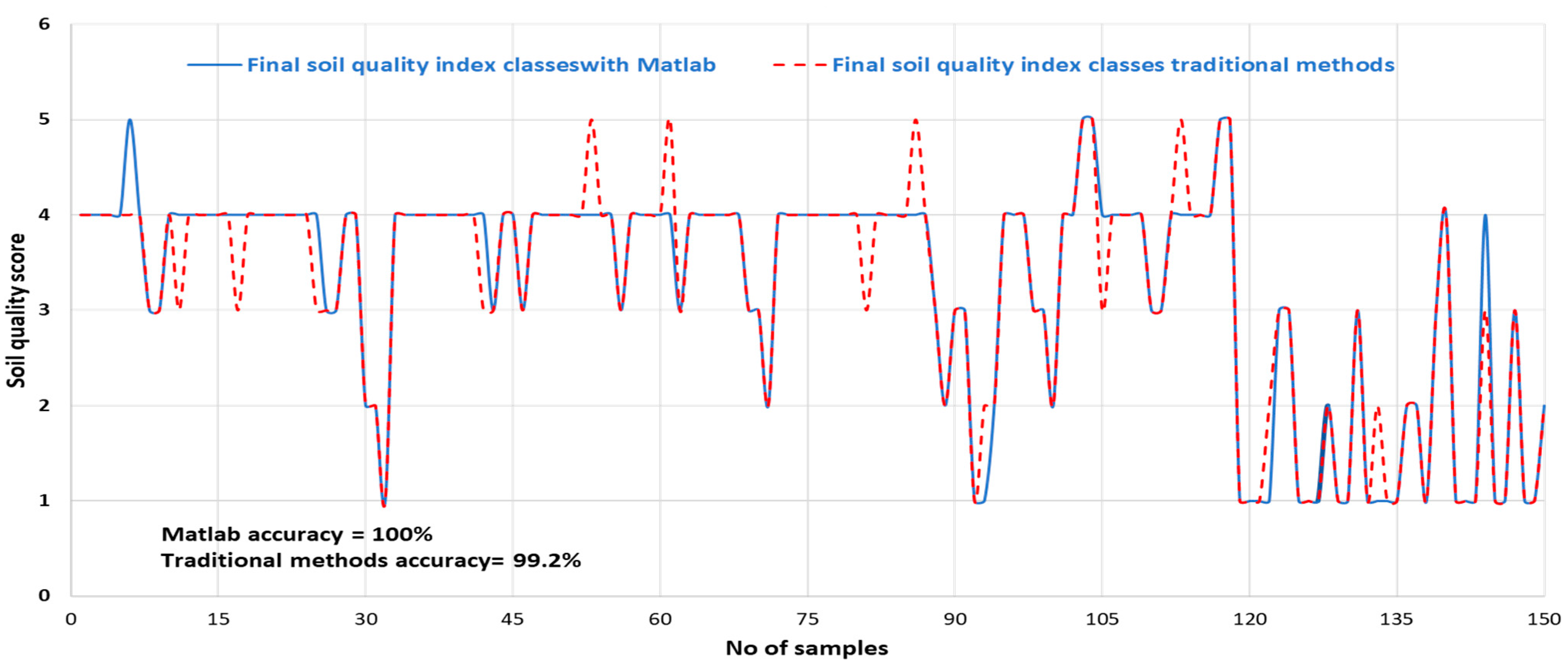
3.2.4. Comparison between the Final Soil Quality Index Class Calculations Using Matlab and Traditional Methods

This study is concerned with comparing the accuracy and efficiency of final soil quality index class calculations using traditional methods and MATLAB. The results, presented in Table 2, reveal that the MATLAB program proposed in the study is highly effective, precise, and fast in processing large amounts of data required for machine learning training.

3.3. ANN Training Phase

The performance of the soil quality prediction program is examined by processing a predefined range of MATLAB output results.
Soil samples were collected at 306 separate points spaced along the length. These values were fed into the feed-forward neural network without performing any preprocessing. According to the literature, the ANN model is suitable for soil quality estimation using multilayer sensory perception with 16 input neurons in one hidden layer and one output, as shown in Figure 9.
In applications involving ANN systems, a low MSE (mean square error) value is typically sufficient. However, to prevent any misestimation of the soil quality index while using ANN systems, a high degree of accuracy in the soil quality index is necessary. The number of neurons in the hidden layer is chosen based on MSE observations, resulting in five times the total number [83,84,85,86,87,88].
There were 306 vector sets in the database; 80% of them were simulated vectors that obtain a low enough training error, and the remaining 20% was kept for the testing step. The ANN training parameters are compiled in Table 3.
Figure 10 presents a comparison of the six models, which allows determination of the best number of neurons for the hidden layer. This provides the activation function with the opportunity to characterize accurately the relationship between input and output. For the training algorithms used in this study, the sigmoidal function is chosen for the hidden layer. Additionally, Figure 10 displays the best training performance over 1000 epochs.
Table 4 presents a comparison of the artificial neural network (ANN) performance with various numbers of hidden layer neurons. The results from the analysis in Table 4 and Figure 10 reveal that the lowest MSE (7.918 × 10⁻²) value during training is achieved using 200 neurons in the hidden layer. However, during the test phase, the MSE (1.856 × 10⁻¹) value is the greatest in the case of 200 neurons. While a low MSE (0.0001) value is sufficient in many applications [78], it is essential to minimize the soil quality estimator’s error to avoid misestimating the true final soil quality index value while using the ANN system.
Based on Figure 10a, which shows the performance of ANN with 50 neurons in the hidden layer, the MSE for training and testing is (0.00857) and (0.01385), respectively. This indicates that the mean square error (MSE) for the training and testing performance exceeded the validation performance (0.0001). This pattern is noticeable in Figure 10b–e, which covers the performance of ANN with 50, 100, 150, 200, and 260 neurons. However, the best performance was achieved with 250 neurons in the hidden layer, as demonstrated in Figure 10e, that presents the actual performance structure for MSE and regression prediction. The Bayesian back-propagation algorithm is used to advance the training states while cross-checking the output and target of the analysis using the ANN. The performance of the chosen epoch describes the best-fit value, while the MSE shows the deviation of the estimated Figure 10e. The validation of 1000 epochs obtained the best results.
In the test phase, Table 4 displays the lowest mean squared error (MSE) of 9.880 × 10⁻². This is achieved by using 250 neurons in the hidden layer, with the best performance occurring at 327 epochs. The reason for this optimal result is due to the large amount of data in the training set, in addition to the high level of accuracy necessary for this application. To achieve this level of accuracy, a large number of neurons is necessary.
Table 5 below shows the ANN training progress and various ANN parameters, number of epochs, elapsed time, performance, gradient, mutation (Mu), and validation checks.
Figure 11 demonstrates that gradient referring to the slope of a line, and in this context, it is most likely referring to the slope of a curve that is plotted during the machine learning model’s training. At epoch 327, the gradient’s value is ‘0.017214’, the numerical value of the slope at that epoch. Epoch refers to a complete pass of all training data in a machine learning model. Therefore, at epoch 327, the model has completed 327 full passes through the training data.
The ‘training state’ of ANN refers to its current stage in the process of training the network to perform a specific task. ANN are trained using a dataset that consists of input data and corresponding desired output data. The process of training ANN involves adjusting the network’s weights and biases of the connections to minimize the difference between the network’s output and the desired output, as shown in Figure 11.
Figure 12 displays a histogram indicating the error for the 20 bins used in performing testing and normalizing data training. The hidden layer achieves the best fit at epoch 1000, resulting in an error value close to zero. This indicates that the predicted values are approximately very close to the actual data. The error histogram confirms the results of both the testing and training phases.
Figure 13 shows the correlation between the estimated actual values plotted on the x-axis and the recorded values on the y-axis for all data, both testing and training. The coefficient of determination (R2) is a useful indicator for evaluating the performance of the proposed artificial neural networks. As shown in Figure 13, the regression for training and test is equal to 0.9651 and 0.9665, respectively, and the overall regression is equal to 0.96502. This means that we can obtain the best accuracy of predictable soil quality by using physical, chemical, and soil fertility parameters.

3.4. ANN Test Phase

In this section, we evaluate the performance of the ANN algorithm for different soil sample features in the test phase. We used a MATLAB-based expert ANN system that takes input signals of soil quality features. Figure 14 shows the histogram in the test phase, which indicates that there are no errors at any point.
Figure 15 is a helpful indicator, as it shows the regression in the test phase. The coefficient of determination (R2) is used to evaluate the performance of the artificial neural networks in predicting soil quality accurately [21]. This proves that the proposed ANN soil quality prediction algorithm is effective, based on the physical, chemical, and fertility soil parameters.

3.5. Assessment of Soil Quality

According to the findings, as shown in Table 6, the FSQI classes are grouped into five quality levels: high (C1 and C2), moderate (C3), and low (C4 and C5). These levels indicate the dominant limitations for ecosystem functions [108]. More than one-third of the overall soil sample quality index, nearly 37%, are classified as very high quality class, whilst only around 0.33% are classified as very low quality class. Additionally, 31.37% of the samples belong to the moderate quality class, 20.92% belong to the low quality class, and the last remaining samples (10.46%) belong to the high quality class. These classes can be associated with limitation factors in certain areas, such as high contents of CaCO3, high pH, high sodium saturation, high salinity, and soil texture (clay content). C5 has a high content of CaCO3 and pH therefore, this soil cannot be cultivated consistently, due to the management process of agriculture being difficult [109]. Moreover, soil reaction and calcium carbonate content affect significant changeability on the degree of soil improvement, in the parent material, gaining or leaching process, and land management applications such as tillage and fertilization systems [110].

4. Conclusions

The increasing demand for soil quality assessment is of great interest to the scientific community for ensuring sustainable use of agricultural land and addressing food security challenges. Machine learning can be used in soil quality assessment and prediction, but it requires precise data from laboratory analyses conducted across diverse zones. A new code has been developed using MATLAB programming language to quickly calculate SQI, and to classify and compile soil sample data into databases. The proposed MATLAB program is highly efficient, accurate, and speedy when handling large data for machine learning training. This reduces the effort, cost, and time required for assessing soil quality.
The use of artificial neural networks (ANN) in machine learning algorithms was investigated to improve learning processes for specific problem areas. The Bayesian back-propagation algorithm was used in this case study to advance training states while cross-checking output target analysis using ANN. In order to achieve the optimal architecture for ANN, the number of neurons was gradually increased to minimize the mean squared error (MSE) during both the training and testing phases. According to this study, the most accurate number of neurons in the hidden layer was 250 neurons. As a result, ANN achieved high coefficient of determination (R2) values for prediction with around 0.97 and 0.98 for training and testing, respectively. The study demonstrates that ANN algorithms can effectively predict changes in spatial patterns over large areas, making them valuable for sustainable agriculture practices. One of the main challenges encountered is overfitting in ANN. As a result, future work will include discussions on methods to overcome this overfitting in ANN.
Regular evaluation of soil quality plays a crucial role in maintaining high crop yields and reducing the gap between production and consumption. Therefore, a proposed methodology can be easily applied to other regions. This approach can aid decision-makers and regional governments in identifying the best ways to enhance soil quality, implement effective soil management practices, and overcome the food security challenge. This challenge is considered one of the most important issues in the 2030 Agenda for Sustainable Development. In future research, soil quality should be assessed with various activation functions and algorithms, and the model should be tested for larger areas. In this case, in addition to guiding future studies, this study could be further improved by adding various biophysical indicators and socio-economic factors.

Supplementary Materials

The following supporting information can be downloaded at: https://www.mdpi.com/article/10.3390/agriculture14040627/s1, Figure S1: Location of study areas.; Table S1: Scores of chemical property parameters; Table S2: Scores of physical property parameters; Table S3: Scores of fertility property parameters; Table S4: Final SQ range of study area.

Author Contributions

Conceptualization, R.A.E.B., H.M.E.A. and M.S.S.; methodology, R.A.E.B., H.M.E.A. and M.S.S.; software. R.A.E.B., H.M.E.A. and M.S.S.; validation, R.A.E.B., H.M.E.A., and M.S.S. formal analysis R.A.E.B., H.M.E.A. and M.S.S.; investigation, R.A.E.B., H.M.E.A. and M.S.S.; resources, R.A.E.B., E.S.M. and M.S.S.; data curation, R.A.E.B., H.M.E.A. and M.S.S.; writing—original draft preparation, R.A.E.B., H.M.E.A. and M.S.S.; writing—review and editing, A.A.E.B., M.M.I. and N.Y.R.; supervision, A.A.E.B., M.M.I. and M.S.S. All authors have read and agreed to the published version of the manuscript.

Funding

This research received no external funding.

Institutional Review Board Statement

Not applicable.

Data Availability Statement

Data are contained within the article or Supplementary Materials. The data presented in this study are available in (Supplementary Materials here).

Acknowledgments

Soil and plant water analysis laboratory team, Faculty of Agriculture, Tanta University. This paper was supported by the RUDN University Strategic Academic Leadership Program.

Conflicts of Interest

The authors declare no conflicts of interest.

References

  1. Hunter, M.C.; Smith, R.G.; Schipanski, M.E.; Atwood, L.W.; Mortensen, D.A. Agriculture in 2050: Recalibrating targets for sustainable intensification. Bioscience 2017, 67, 386–391. [Google Scholar] [CrossRef]
  2. Tahmasebinia, F.; Tsumura, Y.; Wang, B.; Wen, Y.; Bao, C.; Sepasgozar, S.; Alonso-Marroquin, F. Floating Cities Bridge in 2050. In Smart Cities and Construction Technologies; IntechOpen: London, UK, 2020; p. 35. [Google Scholar]
  3. Shokr, M.S.; Abdellatif, M.A.; El Baroudy, A.A.; Elnashar, A.; Ali, E.F.; Belal, A.A.; Attia, W.; Ahmed, M.; Aldosari, A.A.; Szantoi, Z. Development of a spatial model for soil quality assessment under arid and semi-arid conditions. Sustainability 2021, 13, 2893. [Google Scholar] [CrossRef]
  4. Hendawy, E.; Belal, A.; Mohamed, E.; Elfadaly, A.; Murgante, B.; Aldosari, A.A.; Lasaponara, R. The prediction and assessment of the impacts of soil sealing on agricultural land in the North Nile Delta (Egypt) using satellite data and GIS modeling. Sustainability 2019, 11, 4662. [Google Scholar] [CrossRef]
  5. Ma, J.; Chen, Y.; Zhou, J.; Wang, K.; Wu, J. Soil quality should be accurate evaluated at the beginning of lifecycle after land consolidation for eco-sustainable development on the Loess Plateau. J. Clean. Prod. 2020, 267, 122244. [Google Scholar] [CrossRef]
  6. Semenkov, I.; Koroleva, T. Heavy metals content in soils of Western Siberia in relation to international soil quality standards. Geoderma Reg. 2020, 21, e00283. [Google Scholar] [CrossRef]
  7. Diaz-Gonzalez, F.A.; Vuelvas, J.; Correa, C.A.; Vallejo, V.E.; Patino, D. Machine learning and remote sensing techniques applied to estimate soil indicators—Review. Ecol. Indic. 2022, 135, 108517. [Google Scholar] [CrossRef]
  8. Bakhshandeh, E.; Hossieni, M.; Zeraatpisheh, M.; Francaviglia, R. Land use change effects on soil quality and biological fertility: A case study in northern Iran. Eur. J. Soil Biol. 2019, 95, 103119. [Google Scholar] [CrossRef]
  9. Zeraatpisheh, M.; Bakhshandeh, E.; Hosseini, M.; Alavi, S.M. Assessing the effects of deforestation and intensive agriculture on the soil quality through digital soil mapping. Geoderma 2020, 363, 114139. [Google Scholar] [CrossRef]
  10. Shao, W.; Guan, Q.; Tan, Z.; Luo, H.; Li, H.; Sun, Y.; Ma, Y. Application of BP-ANN model in evaluation of soil quality in the arid area, northwest China. Soil Tillage Res. 2021, 208, 104907. [Google Scholar] [CrossRef]
  11. Jian, J.; Du, X.; Reiter, M.S.; Stewart, R.D. A meta-analysis of global cropland soil carbon changes due to cover cropping. Soil Biol. Biochem. 2020, 143, 107735. [Google Scholar] [CrossRef]
  12. Guo, L.; Sun, Z.; Ouyang, Z.; Han, D.; Li, F. A comparison of soil quality evaluation methods for Fluvisol along the lower Yellow River. Catena 2017, 152, 135–143. [Google Scholar] [CrossRef]
  13. Zhang, Z.; Han, J.; Yin, H.; Xue, J.; Jia, L.; Zhen, X.; Chang, J.; Wang, S.; Yu, B. Assessing the effects of different long-term ecological engineering enclosures on soil quality in an alpine desert grassland area. Ecol. Indic. 2022, 143, 109426. [Google Scholar] [CrossRef]
  14. Kenge, R. Machine Learning, Its Limitations, and Solutions Over IT. Int. J. Inf. Technol. Model. Comput. 2020, 11, 73–83. [Google Scholar] [CrossRef]
  15. Suthaharan, S. Machine learning models and algorithms for big data classification. Integr. Ser. Inf. Syst 2016, 36, 1–12. [Google Scholar]
  16. Cravero, A.; Pardo, S.; Sepúlveda, S.; Muñoz, L. Challenges to Use Machine Learning in Agricultural Big Data: A Systematic Literature Review. Agronomy 2022, 12, 748. [Google Scholar] [CrossRef]
  17. Liakos, K.G.; Busato, P.; Moshou, D.; Pearson, S.; Bochtis, D. Machine learning in agriculture: A review. Sensors 2018, 18, 2674. [Google Scholar] [CrossRef] [PubMed]
  18. Shi, T.; Zhang, J.; Shen, W.; Wang, J.; Li, X. Machine learning can identify the sources of heavy metals in agricultural soil: A case study in northern Guangdong Province, China. Ecotoxicol. Environ. Saf. 2022, 245, 114107. [Google Scholar] [CrossRef] [PubMed]
  19. Ismaili, M.; Krimissa, S.; Namous, M.; Htitiou, A.; Abdelrahman, K.; Fnais, M.S.; Lhissou, R.; Eloudi, H.; Faouzi, E.; Benabdelouahab, T. Assessment of soil suitability using machine learning in arid and semi-arid regions. Agronomy 2023, 13, 165. [Google Scholar] [CrossRef]
  20. Pant, J.; Pant, P.; Pant, R.; Bhatt, A.; Pant, D.; Juyal, A. Soil quality prediction for determining soil fertility in Bhimtal Block of Uttarakhand (India) using machine learning. Int. J. Anal. Appl. 2021, 19, 91–109. [Google Scholar]
  21. Pacci, S.; Kaya, N.S.; Turan, İ.D.; Odabas, M.S.; Dengiz, O. Comparative approach for soil quality index based on spatial multi-criteria analysis and artificial neural network. Arab. J. Geosci. 2022, 15, 104. [Google Scholar] [CrossRef]
  22. Alaboz, P.; Odabas, M.S.; Dengiz, O. Soil quality assessment based on machine learning approach for cultivated lands in semi-humid environmental condition part of Black Sea region. Arch. Agron. Soil Sci. 2023, 69, 3514–3532. [Google Scholar] [CrossRef]
  23. Shaddad, S.M. Geostatistics and proximal soil sensing for sustainable agriculture. In Sustainability of Agricultural Environment in Egypt: Part I: Soil-Water-Food Nexus; Springer: Cham, Switzerland, 2019; pp. 255–271. [Google Scholar]
  24. Asadi Nalivan, O.; Mousavi Tayebi, S.A.; Mehrabi, M.; Ghasemieh, H.; Scaioni, M. A hybrid intelligent model for spatial analysis of groundwater potential around Urmia Lake, Iran. Stoch. Environ. Res. Risk Assess. 2023, 37, 1821–1838. [Google Scholar] [CrossRef]
  25. Jaiswal, A.; Babu, A.R.; Zadeh, M.Z.; Banerjee, D.; Makedon, F. A survey on contrastive self-supervised learning. Technologies 2020, 9, 2. [Google Scholar] [CrossRef]
  26. Sha, T.; Zhang, W.; Shen, T.; Li, Z.; Mei, T. Deep Person Generation: A Survey from the Perspective of Face, Pose, and Cloth Synthesis. ACM Comput. Surv. 2023, 55, 1–37. [Google Scholar] [CrossRef]
  27. Lin, L.-J. Self-improving reactive agents based on reinforcement learning, planning and teaching. Mach. Learn. 1992, 8, 293–321. [Google Scholar] [CrossRef]
  28. Monjardin, C.E.F.; Power, C.; Senoro, D.B.; De Jesus, K.L.M. Application of Machine Learning for Prediction and Monitoring of Manganese Concentration in Soil and Surface Water. Water 2023, 15, 2318. [Google Scholar] [CrossRef]
  29. Kolassa, J.; Reichle, R.; Liu, Q.; Alemohammad, S.; Gentine, P.; Aida, K.; Asanuma, J.; Bircher, S.; Caldwell, T.; Colliander, A. Estimating surface soil moisture from SMAP observations using a Neural Network technique. Remote Sens. Environ. 2018, 204, 43–59. [Google Scholar] [CrossRef] [PubMed]
  30. Ng, W.; Minasny, B.; Montazerolghaem, M.; Padarian, J.; Ferguson, R.; Bailey, S.; McBratney, A.B. Convolutional neural network for simultaneous prediction of several soil properties using visible/near-infrared, mid-infrared, and their combined spectra. Geoderma 2019, 352, 251–267. [Google Scholar] [CrossRef]
  31. El-Sayed, M.A.; Abd-Elazem, A.H.; Moursy, A.R.; Mohamed, E.S.; Kucher, D.E.; Fadl, M.E. Integration Vis-NIR Spectroscopy and Artificial Intelligence to Predict Some Soil Parameters in Arid Region: A Case Study of Wadi Elkobaneyya, South Egypt. Agronomy 2023, 13, 935. [Google Scholar] [CrossRef]
  32. Alqadhi, S.; Mallick, J.; Talukdar, S.; Alkahtani, M. An artificial intelligence-based assessment of soil erosion probability indices and contributing factors in the Abha-Khamis watershed, Saudi Arabia. Front. Ecol. Evol. 2023, 11, 1189184. [Google Scholar] [CrossRef]
  33. Suo, X.M.; Jiang, Y.T.; Mei, Y.A.; Li, S.K.; Wang, K.R.; Wang, C.T. Artificial neural network to predict leaf population chlorophyll content from cotton plant images. Agric. Sci. China 2010, 9, 38–45. [Google Scholar] [CrossRef]
  34. Kinhal, V.G.; Agarwal, P.; Gupta, H.O. Performance investigation of neural-network-based unified power-quality conditioner. IEEE Trans. Power Deliv. 2010, 26, 431–437. [Google Scholar] [CrossRef]
  35. Khalghani, M.R.; Khooban, M.H. A novel self-tuning control method based on regulated bi-objective emotional learning controller’s structure with TLBO algorithm to control DVR compensator. Appl. Soft Comput. 2014, 24, 912–922. [Google Scholar] [CrossRef]
  36. Bhat, S.A.; Huang, N.-F. Big data and ai revolution in precision agriculture: Survey and challenges. IEEE Access 2021, 9, 110209–110222. [Google Scholar] [CrossRef]
  37. Mazza, D.; Canuto, E. Fundamental Chemistry with Matlab; Elsevier: Amsterdam, The Netherlands, 2022. [Google Scholar]
  38. Arinze Emmanuel, E.; Okafor Chukwuma, C. A Matlab® Program for Soil Classification Using Aashto Classification. IOSR J. Mech. Civ. Eng. 2015, 12, 58–62. [Google Scholar]
  39. Pawar, S.B.; Kolhe, P.; Jadhav, V.; Patil, A.; Gujar, B.; Bhange, H. Application of C programming language to determine soil phase relationship. Pharma Innov. J. 2022, SP-11, 1835–1841. [Google Scholar]
  40. Raorane, A.A.; Kulkarni, R.V. Role of MATLAB in Crop Yield Estimation. Int. J. Sci. Res. Comput. Sci. (IJSRCS) 2014, 2, 1–8. [Google Scholar]
  41. Abdellatif, M.A. A Remote Sensing and GIS Techniques Based Approach for the Quantitative Assessment of Soil Quality in Some Areas of Northwestren Coast. Ph.D. Thesis, Faculty of Agriculture, Tanta University, Cairo, Egypt, 2022. [Google Scholar]
  42. El-Baroudy, A.A. Using Remote Sensing and GIS Techniques for Monitoring Land Degradation in Some Areas of Nile Delta. Ph.D. Thesis, Faculty of Agriculture, Tanta University, Cairo, Egypt, 2005. [Google Scholar]
  43. El Behairy, R.A. Using New Techniques for Studying Land Resources in Some Areas of North West Nile Delta, Egypt. Master’s Thesis, Faculty of Agriculture, Tanta University, Cairo, Egypt, 2021. [Google Scholar]
  44. Food, Agriculture Organization of the United Nations Soil Resources Development and Conservation Service. Guidelines for Soil Profile Description; FAO Soil Resources Development and Conservation Service: Rome, Italy, 2006. [Google Scholar]
  45. Taxonomy, S. Keys to Soil Taxonomy; United State Department of Agriculture (USDA), Natural Resources Conservation Service: Washington, DC, USA, 2014.
  46. Usda, N. Soil survey laboratory methods manual. In Soil Survey Investigations Report; Department of Agriculture, Natural Resources Conservation Service: Lincoln, NE, USA, 2004; No. 42. [Google Scholar]
  47. Read, S. ISO/IEC 17025; 2017-General requirements for the competence of testing and calibration laboratories. Vernier: Geneva, Switzerland, 2017.
  48. Karlen, D.L.; Ditzler, C.A.; Andrews, S.S. Soil quality: Why and how? Geoderma 2003, 114, 145–156. [Google Scholar] [CrossRef]
  49. El Behairy, R.A.; El Baroudy, A.A.; Ibrahim, M.M.; Kheir, A.M.; Shokr, M.S. Modelling and assessment of irrigation water quality index using GIS in semi-arid region for sustainable agriculture. Water Air Soil Pollut. 2021, 232, 352. [Google Scholar] [CrossRef]
  50. Shokr, M.S.; Abdellatif, M.A.; El Behairy, R.A.; Abdelhameed, H.H.; El Baroudy, A.A.; Mohamed, E.S.; Rebouh, N.Y.; Ding, Z.; Abuzaid, A.S. Assessment of Potential Heavy Metal Contamination Hazards Based on GIS and Multivariate Analysis in Some Mediterranean Zones. Agronomy 2022, 12, 3220. [Google Scholar] [CrossRef]
  51. El Behairy, R.A.; El Baroudy, A.A.; Ibrahim, M.M.; Mohamed, E.S.; Kucher, D.E.; Shokr, M.S. Assessment of soil capability and crop suitability using integrated multivariate and GIS approaches toward agricultural sustainability. Land 2022, 11, 1027. [Google Scholar] [CrossRef]
  52. Hammam, A.A.; Mohamed, W.S.; Sayed, S.E.-E.; Kucher, D.E.; Mohamed, E.S. Assessment of soil contamination using gis and multi-variate analysis: A case study in El-Minia Governorate, Egypt. Agronomy 2022, 12, 1197. [Google Scholar] [CrossRef]
  53. El Behairy, R.A.; El Baroudy, A.A.; Ibrahim, M.M.; Mohamed, E.S.; Rebouh, N.Y.; Shokr, M.S. Combination of GIS and Multivariate Analysis to Assess the Soil Heavy Metal Contamination in Some Arid Zones. Agronomy 2022, 12, 2871. [Google Scholar] [CrossRef]
  54. Watzinger, A. Microbial phospholipid biomarkers and stable isotope methods help reveal soil functions. Soil Biol. Biochem. 2015, 86, 98–107. [Google Scholar] [CrossRef]
  55. Istijono, B.; Harianti, M. Soil quality index analysis under horticultural farming in Sumani upper watershed. GEOMATE J. 2019, 16, 191–196. [Google Scholar]
  56. Moore, F.; Sheykhi, V.; Salari, M.; Bagheri, A. Soil quality assessment using GIS-based chemometric approach and pollution indices: Nakhlak mining district, Central Iran. Environ. Monit. Assess. 2016, 188, 214. [Google Scholar] [CrossRef] [PubMed]
  57. Dengiz, O. Parametric approach with linear combination technique in land evaluation studies. J. Agric. Sci. 2013, 19, 101–112. [Google Scholar]
  58. Şenol, H.; Alaboz, P.; Demir, S.; Dengiz, O. Computational intelligence applied to soil quality index using GIS and geostatistical approaches in semiarid ecosystem. Arab. J. Geosci. 2020, 13, 1–20. [Google Scholar] [CrossRef]
  59. Semih, Ç.; Barik, K. Hydraulic conductivity values of soils in different soil processing conditions. Alinteri J. Agric. Sci. 2020, 35, 132–138. [Google Scholar]
  60. Alam, M.; Mishra, A.; Singh, K.; Singh, S.K.; David, A. Response of sulphur and FYM on soil physico-chemical properties and growth, yield and quality of mustard (Brassica nigra L.). J. Agric. Phys. 2014, 14, 156–160. [Google Scholar]
  61. Fabrizio, A.; Tambone, F.; Genevini, P. Effect of compost application rate on carbon degradation and retention in soils. Waste Manag. 2009, 29, 174–179. [Google Scholar] [CrossRef]
  62. Palmer, J.; Thorburn, P.J.; Biggs, J.S.; Dominati, E.J.; Probert, M.E.; Meier, E.A.; Huth, N.I.; Dodd, M.; Snow, V.; Larsen, J.R. Nitrogen cycling from increased soil organic carbon contributes both positively and negatively to ecosystem services in wheat agro-ecosystems. Front. Plant Sci. 2017, 8, 731. [Google Scholar] [CrossRef] [PubMed]
  63. Ramos, F.T.; Dores, E.F.d.C.; Weber, O.L.d.S.; Beber, D.C.; Campelo Jr, J.H.; Maia, J.C.d.S. Soil organic matter doubles the cation exchange capacity of tropical soil under no-till farming in Brazil. J. Sci. Food Agric. 2018, 98, 3595–3602. [Google Scholar] [CrossRef] [PubMed]
  64. Alaboz, P.; Dengiz, O.; Demir, S. Barley yield estimation performed by ANN integrated with the soil quality index modified by biogas waste application. Zemdirb. Agric. 2021, 108, 217–226. [Google Scholar] [CrossRef]
  65. Shokr, M.S.; Baroudy, A.A.E.L.; Fullen, M.A.; El-Beshbeshy, T.R.; Ali, R.R.; Elhalim, A.; Guerra, A.J.T.; Jorge, M.C.O. Mapping of Heavy Metal Contamination in Alluvial Soils of the Middle Nile Delta of Egypt. J. Environ. Eng. Landsc. Manag. 2016, 24, 218–231. [Google Scholar] [CrossRef]
  66. Abdellatif, M.A.; El Baroudy, A.A.; Arshad, M.; Mahmoud, E.K.; Saleh, A.M.; Moghanm, F.S.; Shaltout, K.H.; Eid, E.M.; Shokr, M.S. A GIS-based approach for the quantitative assessment of soil quality and sustainable agriculture. Sustainability 2021, 13, 13438. [Google Scholar] [CrossRef]
  67. Abuzaid, A.S.; Abdellatif, A.D.; Fadl, M.E. Modeling soil quality in Dakahlia Governorate, Egypt using GIS techniques. Egypt. J. Remote Sens. Space Sci. 2021, 24, 255–264. [Google Scholar] [CrossRef]
  68. El Behairy, R.A.; El Arwash, H.M.; El Baroudy, A.A.; Ibrahim, M.M.; Mohamed, E.S.; Rebouh, N.Y.; Shokr, M.S. Artificial Intelligence Integrated GIS for Land Suitability Assessment of Wheat Crop Growth in Arid Zones to Sustain Food Security. Agronomy 2023, 13, 1281. [Google Scholar] [CrossRef]
  69. El Baroudy, A. Mapping and evaluating land suitability using a GIS-based model. Catena 2016, 140, 96–104. [Google Scholar] [CrossRef]
  70. Baroudy, A.A.E.; Ali, A.M.; Mohamed, E.S.; Moghanm, F.S.; Shokr, M.S.; Savin, I.; Poddubsky, A.; Ding, Z.; Kheir, A.M.; Aldosari, A.A. Modeling land suitability for rice crop using remote sensing and soil quality indicators: The case study of the nile delta. Sustainability 2020, 12, 9653. [Google Scholar] [CrossRef]
  71. Staff, S. Soil Survey Manual in USDA Handbook 18; Ditzler, C., Scheffe, K., Monger, H.C., Eds.; Government Printing Office: Washington, DC, USA, 2017.
  72. Yao, R.-J.; Yang, J.-S.; Zhang, T.-J.; Gao, P.; Yu, S.-P.; Wang, X.-P. Short-term effect of cultivation and crop rotation systems on soil quality indicators in a coastal newly reclaimed farming area. J. Soils Sediments 2013, 13, 1335–1350. [Google Scholar] [CrossRef]
  73. Abrol, I.; Yadav, J.S.P.; Massoud, F. Salt-Affected Soils and Their Management; Food & Agriculture Organization: Rome, Italy, 1988. [Google Scholar]
  74. Hazelton, P.; Murphy, B. Interpreting Soil Test Results: What Do All the Numbers Mean? CSIRO Publishing: Collingwood, VA, Australia, 2016. [Google Scholar]
  75. Soltanpour, P. Determination of nutrient availability and elemental toxicity by AB-DTPA soil test and ICPS. In Advances in Soil Science; Springer: New York, NY, USA, 1991; Volume 16, pp. 165–190. [Google Scholar]
  76. Mohamed, E.S.; Baroudy, A.A.E.; El-Beshbeshy, T.; Emam, M.; Belal, A.; Elfadaly, A.; Aldosari, A.A.; Ali, A.M.; Lasaponara, R. Vis-nir spectroscopy and satellite landsat-8 oli data to map soil nutrients in arid conditions: A case study of the northwest coast of Egypt. Remote Sens. 2020, 12, 3716. [Google Scholar] [CrossRef]
  77. Mohamed, E.S.; Jalhoum, M.E.; Belal, A.A.; Hendawy, E.; Azab, Y.F.; Kucher, D.E.; Shokr, M.S.; El Behairy, R.A.; El Arwash, H.M. A Novel Approach for Predicting Heavy Metal Contamination Based on Adaptive Neuro-Fuzzy Inference System and GIS in an Arid Ecosystem. Agronomy 2023, 13, 1873. [Google Scholar] [CrossRef]
  78. Salman, M.S.; Kukrer, O.; Hocanin, A. Recursive inverse algorithm: Mean-square-error analysis. Digit. Signal Process. 2017, 66, 10–17. [Google Scholar] [CrossRef]
  79. Sharma, S.; Sharma, S.; Athaiya, A. Activation functions in neural networks. Towards Data Sci. 2017, 6, 310–316. [Google Scholar] [CrossRef]
  80. Fei, R.; Guo, Y.; Li, J.; Hu, B.; Yang, L. An improved BPNN method based on probability density for indoor location. IEICE Trans. Inf. Syst. 2023, 106, 773–785. [Google Scholar] [CrossRef]
  81. Jain, A.K.; Chandrasekaran, B. 39 Dimensionality and sample size considerations in pattern recognition practice. Handb. Stat. 1982, 2, 835–855. [Google Scholar]
  82. Raudys, S.J.; Jain, A.K. Small sample size effects in statistical pattern recognition: Recommendations for practitioners. IEEE Trans. Pattern Anal. Mach. Intell. 1991, 13, 252–264. [Google Scholar] [CrossRef]
  83. Dayhoff, J. Pattern recognition with a pulsed neural network. In Proceedings of the Conference on Analysis of Neural Network Applications, Fairfax, VA, USA, 29–31 May 1991; pp. 146–159. [Google Scholar]
  84. Mehrotra, K.; Mohan, C.K.; Ranka, S. Elements of Artificial Neural Networks; MIT Press: Cambridge, MA, USA, 1997. [Google Scholar]
  85. Haykin, S. Neural Networks: A Comprehensive Foundation; Prentice Hall PTR: Hoboken, NJ, USA, 1998. [Google Scholar]
  86. Haykin, S. Neural networks: A guided tour. In Nonlinear Biomedical Signal Processing; Institute of Electrical and Electronics Engineers, Inc.: Piscataway, NJ, USA, 2000; Volume 1, pp. 53–68. [Google Scholar]
  87. Rasmussen, C.E.; Williams, C.K. Gaussian Processes for Machine Learning; Springer: Berlin/Heidelberg, Germany, 2006; Volume 1. [Google Scholar]
  88. Dayhoff, J.E. Neural Network Architectures: An Introduction; Van Nostrand Reinhold Co.: New York, NY, USA, 1990. [Google Scholar]
  89. Mockus, J.; Mockus, J. Global optimization and the Bayesian approach. In Bayesian Approach to Global Optimization: Theory and Applications; Springer: Dordrecht, The Netherlands, 1989; pp. 1–3. [Google Scholar]
  90. Snoek, J.; Larochelle, H.; Adams, R.P. Practical bayesian optimization of machine learning algorithms. In Advances in Neural Information Processing Systems; Morgan Kaufmann Publishers, Inc.: Burlington, MA, USA, 2012; Volume 25. [Google Scholar]
  91. Wu, J.; Chen, X.-Y.; Zhang, H.; Xiong, L.-D.; Lei, H.; Deng, S.-H. Hyperparameter optimization for machine learning models based on Bayesian optimization. J. Electron. Sci. Technol. 2019, 17, 26–40. [Google Scholar]
  92. Shahriari, B.; Swersky, K.; Wang, Z.; Adams, R.P.; De Freitas, N. Taking the human out of the loop: A review of Bayesian optimization. Proc. IEEE 2015, 104, 148–175. [Google Scholar] [CrossRef]
  93. Nachshon, U. Cropland soil salinization and associated hydrology: Trends, processes and examples. Water 2018, 10, 1030. [Google Scholar] [CrossRef]
  94. Hammam, A.; Mohamed, E. Mapping soil salinity in the East Nile Delta using several methodological approaches of salinity assessment. Egypt. J. Remote Sens. Space Sci. 2020, 23, 125–131. [Google Scholar] [CrossRef]
  95. Abdel-Fattah, M.K.; Abd-Elmabod, S.K.; Aldosari, A.A.; Elrys, A.S.; Mohamed, E.S. Multivariate analysis for assessing irrigation water quality: A case study of the Bahr Mouise Canal, Eastern Nile Delta. Water 2020, 12, 2537. [Google Scholar] [CrossRef]
  96. Zalacáin, D.; Martínez-Pérez, S.; Bienes, R.; García-Díaz, A.; Sastre-Merlín, A. Salt accumulation in soils and plants under reclaimed water irrigation in urban parks of Madrid (Spain). Agric. Water Manag. 2019, 213, 468–476. [Google Scholar] [CrossRef]
  97. Qadir, M.; Schubert, S. Degradation processes and nutrient constraints in sodic soils. Land Degrad. Dev. 2002, 13, 275–294. [Google Scholar] [CrossRef]
  98. Jacobsen, S.-E.; Jensen, C.R.; Liu, F. Improving crop production in the arid Mediterranean climate. Field Crops Res. 2012, 128, 34–47. [Google Scholar] [CrossRef]
  99. Osman, K.T. Management of Soil Problems; Springer: Berlin/Heidelberg, Germany, 2018. [Google Scholar]
  100. Von Wandruszka, R. Phosphorus retention in calcareous soils and the effect of organic matter on its mobility. Geochem. Trans. 2006, 7, 6. [Google Scholar] [CrossRef] [PubMed]
  101. Chi, C.; Zhao, C.; Sun, X.; Wang, Z. Reclamation of saline-sodic soil properties and improvement of rice (Oriza sativa L.) growth and yield using desulfurized gypsum in the west of Songnen Plain, northeast China. Geoderma 2012, 187, 24–30. [Google Scholar] [CrossRef]
  102. Temiz, C.; Cayci, G. The effects of gypsum and mulch applications on reclamation parameters and physical properties of an alkali soil. Environ. Monit. Assess. 2018, 190, 347. [Google Scholar] [CrossRef]
  103. Abdelsamie, E.A.; Abdellatif, M.A.; Hassan, F.O.; El Baroudy, A.A.; Mohamed, E.S.; Kucher, D.E.; Shokr, M.S. Integration of RUSLE Model, Remote Sensing and GIS Techniques for Assessing Soil Erosion Hazards in Arid Zones. Agriculture 2022, 13, 35. [Google Scholar] [CrossRef]
  104. Abdel-Fattah, M.K.; Mohamed, E.S.; Wagdi, E.M.; Shahin, S.A.; Aldosari, A.A.; Lasaponara, R.; Alnaimy, M.A. Quantitative evaluation of soil quality using Principal Component Analysis: The case study of El-Fayoum depression Egypt. Sustainability 2021, 13, 1824. [Google Scholar] [CrossRef]
  105. Bassouny, M.; Abuzaid, A. Impact of biogas slurry on some physical properties in sandy and calcareous soils, Egypt. Int. J. Plant Soil Sci. 2017, 16, 1–11. [Google Scholar] [CrossRef]
  106. Abuzaid, A.S.; Jahin, H.S. Profile distribution and source identification of potentially toxic elements in north Nile Delta, Egypt. Soil Sediment Contam. Int. J. 2019, 28, 582–600. [Google Scholar] [CrossRef]
  107. Mammadov, E.; Denk, M.; Riedel, F.; Lewinska, K.; Kaźmierowski, C.; Glaesser, C. Visible and near-infrared reflectance spectroscopy for assessment of soil properties in the Caucasus Mountains, Azerbaijan. Commun. Soil Sci. Plant Anal. 2020, 51, 2111–2136. [Google Scholar] [CrossRef]
  108. Fadl, M.; Abuzaid, A. Assessment of land suitability and water requirements for different crops in Dakhla Oasis, Western Desert, Egypt. Int. J. Plant Soil Sci. 2017, 16, 1–16. [Google Scholar] [CrossRef]
  109. Bernardi, A.C.d.C.; Grego, C.R.; Andrade, R.G.; Rabello, L.M.; Inamasu, R.Y. Spatial variability of vegetation index and soil properties in an integrated crop-livestock system. Rev. Bras. De Eng. Agrícola E Ambient. 2017, 21, 513–518. [Google Scholar] [CrossRef]
  110. Öztürk, E.; Dengiz, O. Assessment and selection of suitable microbasins for organic agriculture under subhumid ecosystem conditions: A case study from Trabzon Province, Turkey. Arab. J. Geosci. 2020, 13, 1222. [Google Scholar] [CrossRef]
Figure 1. Flow chart describing the performed working methodology of this study.
Agriculture 14 00627 g001
Figure 2. Flow chart describing soil quality index calculation using Matlab codes.
Agriculture 14 00627 g002
Figure 3. EC score calculations using MATLAB code.
Agriculture 14 00627 g003
Figure 4. FSQI class calculations using MATLAB code.
Agriculture 14 00627 g004
Figure 5. The Bayesian artificial neural network (ANN) model flow chart.
Agriculture 14 00627 g005
Figure 6. Comparison between the obtained results from traditional methods and the proposed MATLAB program.
Agriculture 14 00627 g006
Figure 7. Comparison between the obtained results from traditional methods and the proposed program.
Agriculture 14 00627 g007
Figure 8. Comparison between the soil quality index calculations using Matlab and traditional methods.
Agriculture 14 00627 g008
Figure 9. ANN model under Matlab.
Agriculture 14 00627 g009
Figure 10. Comparison between the ANN best training performance using various neurons in hidden layer: (a) 50; (b) 100; (c) 150; (d) 200; (e) 250; and (f) 260 neurons.
Agriculture 14 00627 g010
Figure 11. The training state parameters using 250 neurons in the hidden layer over 1000 epochs.
Agriculture 14 00627 g011
Figure 12. The training error histogram for the data using ANN back-propagation.
Agriculture 14 00627 g012
Figure 13. The regression plots depict the correlation between the output data and the targets.
Agriculture 14 00627 g013
Figure 14. The test histogram error.
Agriculture 14 00627 g014
Figure 15. The regression depicts the relation between the output data and the targets.
Agriculture 14 00627 g015
Table 1. Descriptive statistics of soil physicochemical properties (n = 306).
Soil PropertyUnitMinMaxMeanSDCV, %SkewnessKurtosis
ECdSm−10.55129.705.4610.91199.86.7361.33
pH-7.469.218.340.313.70.11−0.05
ESP%1.4535.939.297.5080.71.251.10
CaCO30.2134.429.158.1589.10.94−0.08
CaSO40.079.681.211.32108.52.8912.16
CECcmolcKg−10.9558.4022.0919.8990.00.27−1.75
HCcmhr−10.2933.429.718.5788.20.54−0.88
WHC%3.0153.0423.3219.3082.80.21−1.83
BDgcm−31.161.681.430.128.5−0.46−0.88
SS%0.108.002.041.6078.52.386.91
SDcm30.00150.00110.5236.3932.9−0.20−1.37
SOM%0.012.960.630.67105.41.521.47
AvKmgKg−17.70719.10263.77144.2554.70.01−0.10
AvP2.0938.459.666.6668.91.331.46
AvN3.1098.9128.7826.5092.10.96−0.43
n = number of soil samples; Min = minimum; Max = maximum; SD = standard deviation; CV = coefficient of variation.
Table 2. Comparison of soil quality class calculations using Matlab and traditional methods.
Comparison FaceTime-ConsumingEffectivenessAccuracy
ScenarioTraditional
Methods
MATLAB
Program
Traditional
Methods
MATLAB
Program
Traditional
Methods
MATLAB
Program
Scenario 1; 150 samples18 h5 m90%100%99.2%100%
Scenario 2; 306 samples37 h5 m80%100%97.9%100%
Scenario 3; 700 samples84 h5 m70%100%97.8%100%
Note: h = hours; and m = minutes.
Table 3. ANN training parameters.
I/P No.16Outputs No.1
No. of training samples245Max. training Epochs1000
Hidden layers1Target Regression (R)1
Target MSE0Target error1 × 10−3
Table 4. ANN training performance with different hidden layer neurons.
No. of Neurons for the Hidden Layers50100150200250260
MSE (Training)8.507 × 10−28.033 × 10−21.066 × 10−17.918 × 10−29.0237 × 10−29.651 × 10−2
MSE (Test)1.385 × 10−11.28 × 10−11.285 × 10−11.856 × 10−19.880 × 10−21.424 × 10−1
R (Training)9.668 × 10−19.69 × 10−19.69 × 10−19.694 × 10−19.650 × 10−19.627 × 10−1
R (Test)9.559 × 10−19.518 × 10−19.518 × 10−19.306 × 10−19.664 × 10−19.531 × 10−1
No. of total epochs for best performance565997873147327162
Table 5. ANN training progress.
UnitEpochElapsed TimePerformanceGradientMutation (Mu)Validation Checks
Initial Value0-1636180.005000
Current Value10001:13:350.07920.01510.5000
Objective Value1000-0.001 × 10−71.00 × 10100
Table 6. Classification and evaluation limits of the FSQI in soil samples.
ClassesSymbolValuesNo. of Samples%
Very high qualityC1≥0.6111336.93
high qualityC20.53–0.603210.46
Moderate qualityC30.45–0.529631.37
Low qualityC40.37–0.446420.92
Very low qualityC5≤0.3610.33
Total306100
Disclaimer/Publisher’s Note: The statements, opinions and data contained in all publications are solely those of the individual author(s) and contributor(s) and not of MDPI and/or the editor(s). MDPI and/or the editor(s) disclaim responsibility for any injury to people or property resulting from any ideas, methods, instructions or products referred to in the content.

