1. Introduction
Precision agriculture (PA) is a new paradigm in agriculture that dates back to the middle of the 1980s [
1] and is experiencing exponential growth, being considered as the one of the top ten revolutions in agriculture [
1,
2]. For example, in the recent past, the number of research works related to PA has increased enormously. A simple search in Google Academics with the term “precision agriculture” returns 2130 records for 2005, 5670 for 2015, and 6670 for 2017. In terms of farmers as well as food and agricultural companies, progressively more and more users are starting to use some kind of PA-based system [
3]. Many of them are focused on automation of agricultural tasks, remote sensing crop monitoring (e.g., [
4]), and on segmentation of within-field variability to delineate potential management zones [
5,
6]. Nevertheless, although PA is little by little gaining weight in the day-to-day of farms, there is still a big gap between scientific research and real implementation and/or full adoption.
One of the fields of research in PA is the delineation of potential management zones (PMZs; also called site-specific management zones (SSMZs), or simply management zones [
1]). This is an important task in PA because it supposes the identification of areas within a field with different productive potential, allowing the opportunity for differential management to be assessed [
7,
8,
9]. Specifically, site-specific crop management is the management of agricultural crops at a spatial scale smaller than the whole field by considering local variability to cost-effectively maximize crop production and the efficient use of agrichemicals to minimize detrimental environmental impacts [
10]. To identify and delineate PMZs, information about the yield variation pattern is a good starting point [
11]. When yield maps are not available, this delineation is usually performed on the basis of other related (proxy) parameters such as remote sensing multispectral indices, soil mapping units, apparent soil electrical conductivity (ECa), or topography, among others [
12,
13].
To delineate PMZs, cluster analysis is the main used and recommended methodology [
14,
15]. This procedure allows pixel values of different maps to be classified into homogeneous groups (map classes). For this, the user can choose between a hard-type or a fuzzy-type classification algorithm. For example, the
k-means algorithm or the Isodata [
16] are examples of hard classifiers in which each observation (map pixel) can only belong to a single class or cluster. On the other hand, the fuzzy
c-means algorithm, as an example of a fuzzy-type classifier, allows more than one class or cluster to be assigned to each observation, with different membership values of belonging [
8]. The Management Zone Analyst (MZA) software [
17] is an example of successful implementation of this algorithm. In short, 2–6 classes can be created using MZA. The program calculates two coefficients to help the user decide on the optimal solution. This is made based on the degree of separation (or overlap) between the partitioned classes (fuzziness performance index, FPI) and on the amount of disorganisation created by the fuzzy partition (normalized classification entropy, NCE).
One of the extensive crops in which precision management has gained adepts due to economic and environmental considerations is maize (
Zea mays L.) as stated by Jin et al. [
18]. One of the most frequent applications of PA techniques is the use of multi-spectral images to improve in-season N management and yield prediction [
19]. Those applications are very interesting for maize growers, because maize is a high N-demanding crop where insufficient supply of N can result in important economic losses, whereas excessive fertilization implies wasting resources and increasing environmental pollution. Then, to take advantage of the productive potential of different areas within a field, delineation of management zones for variable rate seeding or variable rate fertilization is considered as an opportunity to achieve higher yields while optimizing agricultural inputs, reducing environmental impact.
As mentioned above, geospatial measurement of apparent soil electrical conductivity (ECa) is one of the most reliable and frequently used measurements to characterize within-field variability of edaphic properties to apply site-specific crop management [
20]. In relation to differential management of maize, different research works have used ECa to generate management zones and/or recommendations for spatially variable rate applications of N fertilizer [
21]. However, these zones were not only based on ECa but on other relevant properties such as elevation and slope, or also taking into account soil brightness images [
22]. Other researchers have found that the best predictor of the spatial pattern of yield variability is the aggregation of yield maps from previous years [
23]. Nevertheless, in the absence of yield maps, or when zones within the field are more sensitive to weather conditions fluctuating from one year to the other, the spatial patterns can be derived from within-season remote sensing images. In this respect, other works have demonstrated the effectiveness of remote sensing-based vegetation indices to track phenological changes such as leaf greenness to infer the maize N status and needs, as well as for yield prediction. For example, Maresma et al. [
19,
24] investigated the correlation of different multispectral vegetation indices with the N status at V12 (12 leaves with visible leaf collar) just before tasselling with a single date image. However, other authors point out that good estimator of biomass and yield can be derived from the use of temporal series of remote-sensing images to characterize dynamics of crop canopy throughout the growing and development cycle [
25,
26]. From that, the accumulation of vegetation index values (e.g., the normalized difference vegetation index, NDVI) from the beginning of the biomass accumulation to grain maturity could be a good alternative to yield maps to estimate the within-field variability to finally delineate potential zones for different management practices.
As can be deduced from the above, there is still no accepted protocol or guidelines for establishing potential management zones [
10]. Then, the delineation of potential management zones for differential crop management may have different solutions, since the resulting zones can vary depending on the input variables considered for clustering [
8]. Then, some important questions arise, which many studies sometimes ignore. For example, do the resulting zones reflect the real soil productive potential? Do the proposed class maps give information about the soil and/or environmental properties/conditions that may limit the productive potential? On the other hand, was the farmer’s expert knowledge taken into account in the management zone delineation process? Within precision agriculture research much emphasis has been put on technology, whereas the knowledge that farmers have and ways to explore it have received little attention [
27]. Farmers know which areas of a field are more or less productive, and the use of this knowledge may allow or help in the identification of management zones. Few studies, however, have specifically addressed the use of farmers’ knowledge for that purpose. Schenatto et al. [
28] evaluated the application of farmers’ experience to determine management zones in soybean fields. They found that the use of farmers’ experience could be an efficient and simple tool that could reduce costs in comparison with the traditional method of using stable soil variables and relief. Another interesting experience, although not specifically addressed to the delineation of management zones, analysed how to integrate farmers’ experience-based knowledge in decision support systems, in order to calculate variable N rate application from satellite images [
29]. They found that PA technology must fit doubly the technical needs of farmers and their usual practices to be adopted.
In accordance with this background, the objective of the present work was to propose a methodology that uses the farmers’ expert knowledge to improve the delineation of potential management zones for differential crop management that result from unsupervised clustering. Our hypothesis is that the farmers’ expert knowledge can add highly valuable information which can guide the segmenting of the initial proposed zones. This knowledge can include information on soil and/or local environmental limitations. This information could be also very useful to decide about management actions to be taken to reduce within-field variability.
2. Materials and Methods
2.1. Study Area and Plot Characteristics
The research was carried out in a commercial plot of 45 ha located in the municipality of Tamarite de Litera (Huesca, NE Spain, Latitude 41.75455°, Longitude 0.36386°, WGS84,
Figure 1). The plot was sown with maize (
Zea mays L.) on 16 April 2017 and was harvested on 20 October 2017. The hybrid was DKC6729YG (Monsanto Company, St. Louis, MO, USA), which is a FAO 700 cycle adapted to the conditions of the Ebro Valley, where the farm is located. The average yield was 12.7 t ha
−1. The precedent crop was second-harvest sunflower (
Helianthus annuus L.). The elevation of the plot ranges from 212 to 235 m.a.s.l., with average slopes of 5%, and a maximum of 20%. Soils were classified as Typic Xerorthents, Typic Xerofluvents, and Haplocalcid Xerics [
30]. The plot is irrigated by a centre pivot consisting of six pipe segments of 60-m each, with a total length of 360 m. The outer-most span has a canyon that irrigates an additional length of 25 m.
2.2. Methodological Approach
The idea that motivated the present research was to analyse some of the affordable possibilities that service companies and/or (advanced) farmers have to delineate potential management zones (PMZs) in order to apply precision agriculture in extensive crops. For that, we proposed the delineation of PMZ based on information acquired during the previous crop season to guide management practices for the next one. The information should be easy to obtain by service companies and/or farmers, for example: freely available remote sensing data, elevation data from public digital elevation models, and apparent electrical conductivity as proxy monitoring of soil variability. The resulting PMZs were delineated according to a clustering procedure (see
Section 2.5) using different input data and were validated with the crop yield map obtained at the end of the season. In addition, the farmer’s expert knowledge was considered in order to revise and refine the results, and to identify the causes of within-field variability to propose solutions (see
Section 2.7).
Figure 2 shows the summary of the proposed methodological approach.
2.3. Remote Sensing Data—Sentinel-2 Imagery: Acquisition, Processing, and Vegetation Indices
According to
Figure 2, multispectral images along the maize cycle in 2017 (from sowing to harvest) were acquired and considered to map PMZs as a first option. These images corresponded to Sentinel-2A satellite and were downloaded from the Copernicus Open Access Hub (
https://scihub.copernicus.eu/). Copernicus is the European Union’s Earth Observation Programme, which is coordinated and managed by the European Commission (
http://www.copernicus.eu/).
Table 1 shows the downloaded images with the identifiers, the cloud cover percentage and the maize development stage at image acquisition date according to Ritchie et al. [
31].
Some of the listed images were discarded due to cloud cover affecting the study area (
Table 1). On the other hand, three of the images were downloaded as Level 1C (Top-of-Atmosphere, ToA reflectance), and the rest were Level-2A (Bottom-of-Atmosphere, BoA reflectance). The Level-1C images were converted to Level-2A with the plugin Sen2Cor (
http://step.esa.int/main/third-party-plugins-2/sen2cor) implemented in the open source ESA Sentinel Application Platform (SNAP), which includes the Sentinel-2 Toolbox. Sen2Cor is a processor for Sentinel-2 Level-2A product generation and formatting. It performs the physical atmospheric, terrain, and cirrus correction of ToA Level-1C Sentinel-2 products and creates, among others, BoA reflectance-corrected bands. The output format is equivalent to the Level-1C User Product: georeferenced JPEG 2000 images with bands with three different resolutions: 10, 20, and 60 m.
Table 2 summarizes the basic spectral information about the Sentinel-2A bands acquired by the onboard Multi Spectral Instrument (MSI). More detailed information about the Sentinel-2 mission, satellites, payloads, spectral bands, and products can be found in Drusch et al. [
32].
Only the B04 (Red 664.5 nm, width 38 nm) and B08 (near infrared NIR 835.1 nm, width 145 nm), with 10-m pixel size, were used to calculate the normalized difference vegetation index (NDVI) according to the Equation (1) [
33]. There are other multispectral broad-band vegetation indices available for use in PA that can be calculated from Sentinel-2 bands (for example, normalized difference index bands B04 and B05 (NDI45) [
34], and the red edge inflection point [
35], among others). However, although several limitations have been recognised, it is one of the most frequently used index used to estimate spatial patterns in crop biomass and/or potential crop yield [
1,
25]. In addition, at present it starts to be widely used in PA services for end users.
After calculating the NDVI for each valid image, and following the criteria proposed by González-Gómez et al. [
26], we plotted the average NDVI of the field for each date to identify the date of the green-up and the date of grain maturity (
Figure 3).
The green-up corresponds to the beginning of the growing phase or crop development stage [
36]. The time series of NDVI allowed for the identification of the green-up moment [
26]. Specifically, the green-up does not correspond to any phenological stage. It is a matter of change from pure soil reflectance to the detection of the growing vegetation cover. In the present case study, it corresponded to the stage characterized by the appearance of 2–4 leaves (V2–V4), which was registered in the Sentinel-2A image acquired on 16 May 2017. From this point on, the crop begins a period of rapid growth until plants reach the plateau of maximum canopy cover and start the tasselling phase (V12–VT). In the reproductive growth stages (silking to grain maturity) the NDVI decreases rapidly.
In the present case study, the accumulated NDVI (aNDVI) was calculated between the green-up date (16 May) and the end of the dent stage (13 September) to map the within-field variability of plant vigour. The aNDVI, as proposed by Campos et al. [
25] and González-Gómez [
26], was preferred to map the within-field variability instead of only using indices of a specific date (e.g., just before tasselling) because, according to our experience, the crop development stage in different parts of the plot is not uniform. It can vary according to soil properties, irrigation rates, and other factors. Therefore, at a specific date there can be parts of the plot in stage VT (tasselling) and others that have not yet reached this stage. For this reason, the aNDVI can better represent the variability of the crop development within the plot, since it is not dependent on the different crop stages at a specific time.
2.4. Apparent Electrical Conductivity and Elevation Data
The second option to delineate PMZs was by considering the combination of the aNDVI with a map of the apparent soil electrical conductivity (ECa). For that, an ECa survey was carried out on 20 June 2016 with a Veris 3100 sensor (Veris Technologies Inc., Salina, KS, USA). Veris 3100 uses two coulter pairs to measure ECa at 0–30 cm (shallow ECa) and 0–90 cm (deep ECa) soil depths simultaneously. Data was georeferenced by means of a Trimble AgGPS332 receiver with EGNOS (European Geostationary Navigation Overlay Service) augmentation to obtain differential global position system (DGPS) locations in geographic coordinates WGS84 (EPSG 4326). Negative ECa values were filtered. Then, values above or below ±2.5 standard deviations (SDs) were considered as outliers and were removed from the original raw data according to the criteria of Taylor et al. [
12]. The final ECa data set consisted of 8230 points with shallow and deep readings. These data were interpolated on a 2-m grid by means of ordinary kriging using an exponential semivariogram model. For this purpose, ArcGIS Geostatistical Analyst 10.4 (ESRI, Redlands, CA, USA) was used.
In the present work, and according to Sudduth et al. [
37], we only used the deep ECa data, since it represents the integrated signal for the 0–90 cm soil profile.
To compare ECa values with saturated paste extract electrical conductivity (ECe), ECa original values were first standardized at the reference temperature of 25 °C using a polynomial function proposed by Sheets and Hendrickx [
38]. Then, ECa values at the reference temperature were converted to ECe according to an empirical regression line calculated with data of our own from a close study area (Equation (2), unpublished),
where ECe is the estimated electrical conductivity of the saturated paste extract in dS m
−1 at 25 °C and ECa is the apparent electrical conductivity converted from mS m
−1 to dS m
−1 at 25 °C according to Sheets and Hendrickx [
38]).
In addition to the first two approaches, the third option to delineate PMZ was to consider elevation data as an input variable, together with the aNDVI and the ECa. For this purpose, a publically available 5 × 5 m spatial resolution digital elevation model (DEM) was used. This DEM was produced by the Spanish National Geographic Institute by means of airborne flights using LiDAR (Light Detection and Ranging), with a density of 0.5 points m−2 or higher.
2.5. Clustering Procedure to Delineate Potential Management Zones
For clustering, we selected a fuzzy logic unsupervised classification method (fuzzy
c-means algorithm), implemented in the Management Zone Analyst (MZA) software of the United States Department of Agriculture Agricultural Research Service [
17]. The fuzzy
c-means algorithm allows more than one class or cluster to be assigned to each individual (pixel inside the plot), according to its characteristics and with different membership values. The class in which each pixel obtained the highest score (assignment) was the class which would finally appear on the classified PMZ map (“defuzzification” process).
According to Fridgen et al. [
17], the optimal fuzzy classification of the input data (
n observations) into classes (
c clusters) is the classification which minimizes the objective function J
m (Equation (3)):
where
m is the fuzziness exponent (
m is usually set in the range 1 <
m ≤ 2; in this particular case
m was set to 1.30), (
dij)
2 is the squared distance between observations and centroids (clusters), and
uij is the membership value assigned to pixel
i within the cluster
j.
As it can be seen in Equation (3), the fuzzy
c-means algorithm introduces the use of a weighting exponent (fuzziness exponent), the function of which was to control the degree of overlap established between the classes or clusters. The algorithm also incorporates the concept of distance between points to evaluate the similarity (proximity) between observations and the centroids of each class. In this respect, the distance used in the present research was the Mahalanobis distance, which was calculated through the matrix product (Equation (4)):
where
yi represents the vector of the
ith observation of the data,
vj is the means vector (centroid) corresponding to the cluster
j, and S is the matrix of variances and covariances of the original data. In this way, as a measure of similarity, the use of Mahalanobis distance enabled a “bringing together” or “separation” of the points, taking into consideration the existing degree of correlation between the original variables (aNDVI, ECa, and DEM).
The selection of the most appropriate number of classes was done on the basis of the calculation of two coefficients: the fuzziness performance index (FPI) and the normalized classification entropy (NCE). The FPI measured the degree of separation (or overlap) between the partitioned classes for the original data matrix [
15], and was calculated using Equation (5):
where
c is the number or clusters. FPI values range between 0 and 1. Those values close to 0 were indicative of distinct classes with little overlap between them, while values close to 1 indicated non-distinct classes or, in other words, classes with a very high degree of overlap.
On the other hand, the NCE provided an estimate of the amount of disorganisation created by the fuzzy partition of the data matrix using a specific number of clusters. It was calculated using Equation (6):
where H is the entropy, in which the logarithmic base
a could be any positive integer, with the values of H varying from 0 to log
a (
c). As before, the NCE values close to 0 were indicative of an appropriate classification (or clustering with a higher degree of organisation). The optimum number of clusters was, therefore, the number which managed to minimize the two proposed coefficients, the FPI and NCE.
2.6. Validation of Potential Management Zones
The validation of PMZ was done with yield data acquired at the end of the season. Specifically, yield data were acquired by means of a Trimble Ag FMX yield monitor (Trimble Inc., Sunnyvale, CA, USA) installed in a Fendt 6335 CPL combine harvester. The combine had a cutting width of 5.60 m (8 rows) and was equipped with tilt sensors to correct the effect of slope on the sensor readings. The yield monitor operation principle is based on an optical sensor to measure grain volume flow rate (l s−1) and grain moisture in real time. The system measured the volume of grain harvested and estimates the weight by multiplying the measured volume by the test weight (grain density). In order to get a higher accuracy, the monitor was calibrated with real grain weight from the first load on 20 October 2017 (the day of harvest). The calibration was done following the recommendations prescribed by Trimble and according to the expertise of the experienced combine driver.
Yield monitor data consisted of a set of 43,580 points. Each point contained data related to the effective harvest width (m), the combine forward speed (km h−1), the grain flow rate cm3 s−1, grain yield (kg ha−1), grain moisture (%), grain temperature (°C), and other less relevant measures.
The procedure to obtain the yield map was as follows. First of all, the points with yield equal to zero were removed. Those mainly corresponded to points of combine displacement within the plot without harvesting. Then, the ratio between the average yield of the monitor and the actual average yield from the loads was calculated (
r1). This ratio was used to multiply the yield of each acquired point to adjust it to match the actual yield average. In a second step, adjusted yield values above or below 2.5 SD were considered outliers and were removed from the data set, according to the criteria used in Taylor et al. [
14]. This procedure was repeated twice until a normal distribution of yield data was achieved without variation in the average yield data compared to the actual yield average. Finally, grain yield values per point were converted to the reference grain moisture content of 14% according to Equation (7).
where Yr is the grain yield at 14% moisture content, Hg is the moisture content provided by the monitor, and Hr is the reference moisture content (14% in the present case).
After data filtering, the final set of yield points consisted of 38,507 points, which were used to interpolate to a continuous grid. This process was performed with VESPER (Variogram Estimation and Spatial Prediction plus Error) [
39], using ordinary kriging in 20 m blocks and projecting interpolated data over a regular 5-m grid. A global variogram of raw data was initially fitted using the exponential model, and a minimum of 90 and a maximum of 100 neighbouring yield data points were used to interpolate each point in the grid.
To check the suitability of PMZ to discriminate areas of different potential yield, an analysis of variance (ANOVA) was performed for each clustering to assess its effect on yield taking the number of classes as factor levels. For that purpose, 80 sample points were randomly distributed within the plot and sampled with respect to yield, the aNDVI class, the aNDVI-ECa class, and the aNDVI-ECa-elevation class. The software JMP Pro 13 (SAS Institute Inc., Cary, NC, USA) was used to perform this data analysis.
2.7. Refinement of Potential Management Zones: Adding Farmer’s Expert Knowledge
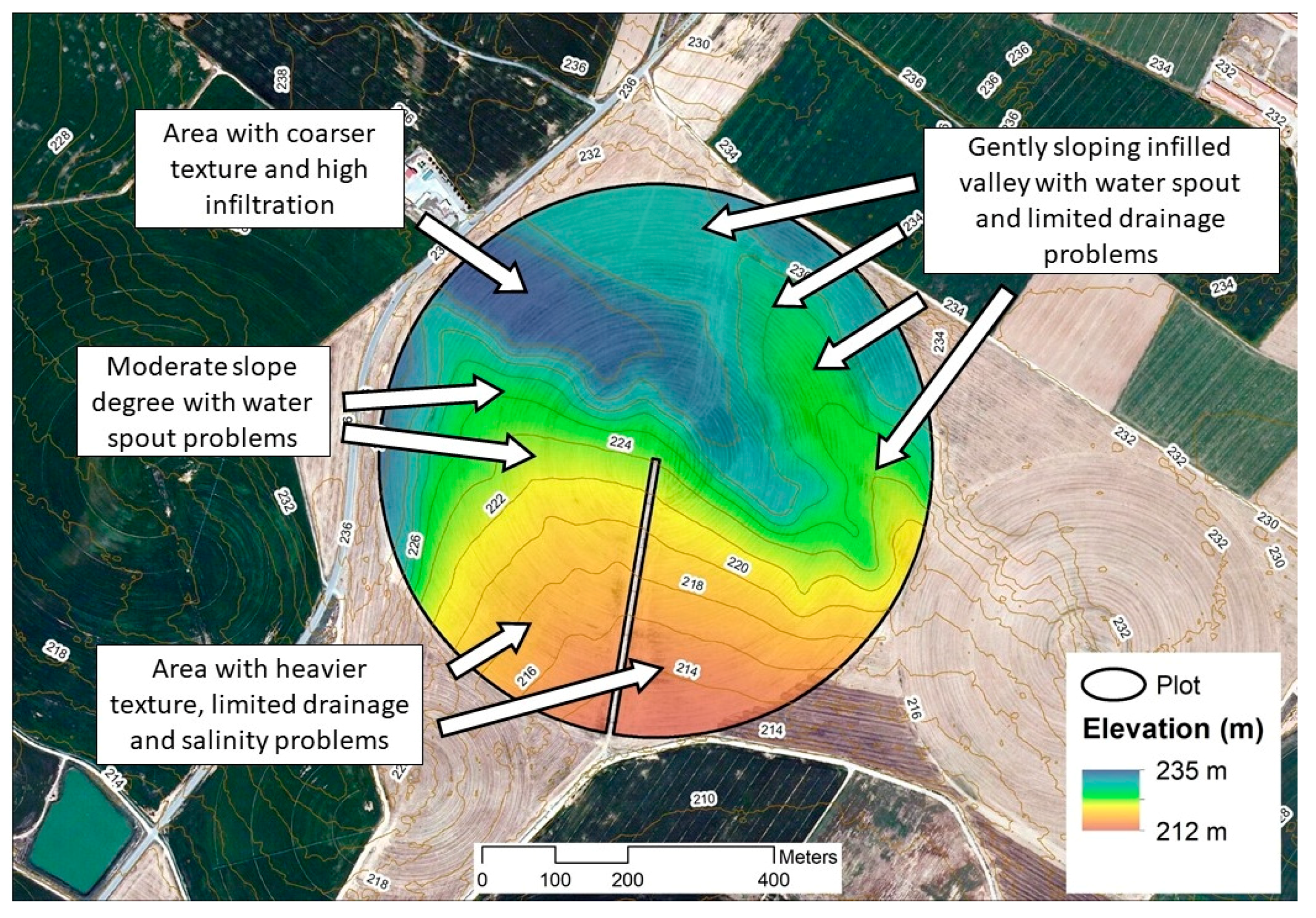
Once the clustering option that best matched with the final yield was selected, a refinement of the zones according to the farmer’s expert knowledge was proposed. The objective was double. First, to avoid a very fragmented map of PMZs, which could complicate the application of differential management actions (e.g., addition of cow manure, variable-rate-application of fertilizers, etc.), and second, associate to the zones the farmer’s knowledge of the possible causes of variability. In this respect, we tried to follow the concept of “on-farm experimentation” built around the farmer’s experiences, observation and analysis of farm operations [
40]. In the present case study, the farmer had 25 years of experience in the farm. This knowledge is summarized in
Figure 4, making use of the elevation map to facilitate the reader with an understanding of the subsequent revision of PMZs presented in the results section. As mentioned above, such expert knowledge was also used to recommend solutions to reduce the within-field variability.
4. Discussion
This research work showed different aspects of within-field variability and zoning that are worth discussing. First, the results revealed an inverse relationship between the accumulated NDVI along the maize cycle and the ECa, and between the yield and ECa. The explanation was the higher values of electrical conductivity in relation to the tolerance level of maize. This is in agreement with the theoretical framework of soil electrical conductivity [
10,
37], which indicates that for saline soils most of the variation in ECa can be related to salt concentration, but in non-saline soils, conductivity variations are primarily a function of soil texture, moisture content, and cation exchange capacity (CEC). However, the highly productive potential zones in the plot (with high aNDVI) mainly corresponded to the lowest ECa values, which in the case of non-saline soils was not expected [
37]. In the present case, the lowest ECa values corresponded to coarse-texture soils which are located in the upper part of the plot and have very good drainage. In good conditions of water supply and fertilization, these soils are the most productive within the plot.
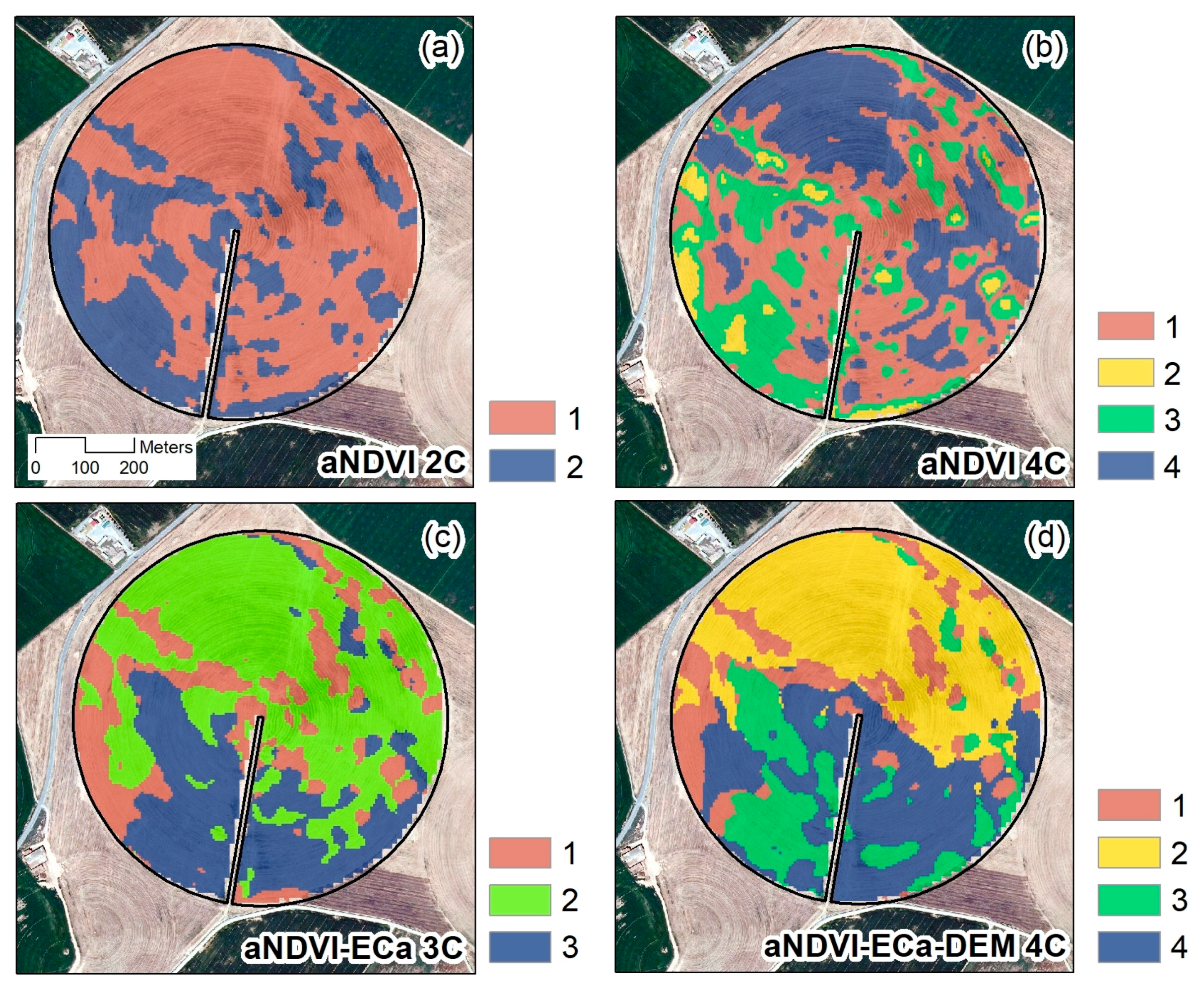
Regarding the unsupervised clustering results, the classification of the accumulated NDVI presented no agreement between the fuzziness performance index (FPI) and the normalized classification entropy (NCE). The two indices indicated different numbers of recommended classes. The ANOVA of the maize yield according to previously delimited classes indicated that the best option was the classification into two classes instead of four. This result is in agreement with the recommendation of Lark and Stafford [
43] and Arnó et al. [
11], who found that the best option is to choose the lowest number of classes.
Clustering the aNDVI in combination with the ECa into three classes did not produce a clear separation of yield levels (
Table 5). Having sorted the classes according to the accumulated NDVI values, there was a class with medium yield (13.1 t ha
−1) and high average ECa (65.9 mS m
−1) and another class with low yield (11.8 t ha
−1) and low average ECa (21.4 mS m
−1). Moreover, similar average ECa values (Class 2 and Class 1 in
Table 5) had very different yields (15.3 and 11.8 t ha
−1, respectively). This reveals that factors other than soil properties could have affected maize growth in areas within Class 1. In the case study plot, these areas suffered a problem of drainage water upwelling coming from the upper parts of the plot (
Figure 4). As is known, excess moisture can produce root hypoxia, which can be one of the major production constrains for maize [
44].
Assessing PMZs resulting from the combined classification of aNDVI, ECa, and DEM, the latter did not seem to be useful in segmenting four yield classes as recommended by the FPI and NCE indices. A priori, the hypothesis could be that the lower parts had to be less productive than the higher parts due to limited drainage and salinity. However, as shown in
Table 5, yield was very different in Classes 1 and 2 characterized by the same high average in elevation, which indicates that topography is not a good discriminant variable to delineate potential management zones, at least in the plot under study. This finding is in contradiction with other works, as in the one by Fraisse et al. [
12], who analysed the “goodness” of PMZ using ECa and topographical data, indicating that elevation and ECa showed better behaviour than slope and a topographic index in defining soil potential management zones.
The accumulated NDVI has been shown to be a good yield predictor, but neither the aNDVI map nor the yield map itself provides information about the cause of spatial variability. In this sense, ECa survey is useful to detect problems of salinity or fine textures that can lead to drainage problems [
13,
37]. In this respect, information revealed as very useful was the farmer’s expert knowledge. There are few works in the literature relating farmer knowledge to precision agriculture, but they have shown interesting results in agreement with the present research. For example, Oliver et al. [
45] integrated farmer’s knowledge and spatial data to define yield zones where targeted soil sampling and crop simulation were then used to determine yield potential and particular constraints. The results provided farmers with a good method for making decisions about spatial management in their fields. Also, Heijting et al. [
27] stated that, given the farmers’ spatial knowledge of their fields, that knowledge is a good starting point to map the within-field variation of soil properties. The results of this work corroborate this concept, highlighting that farmer’s knowledge cannot be ignored and should be considered as an important information source in precision agriculture.
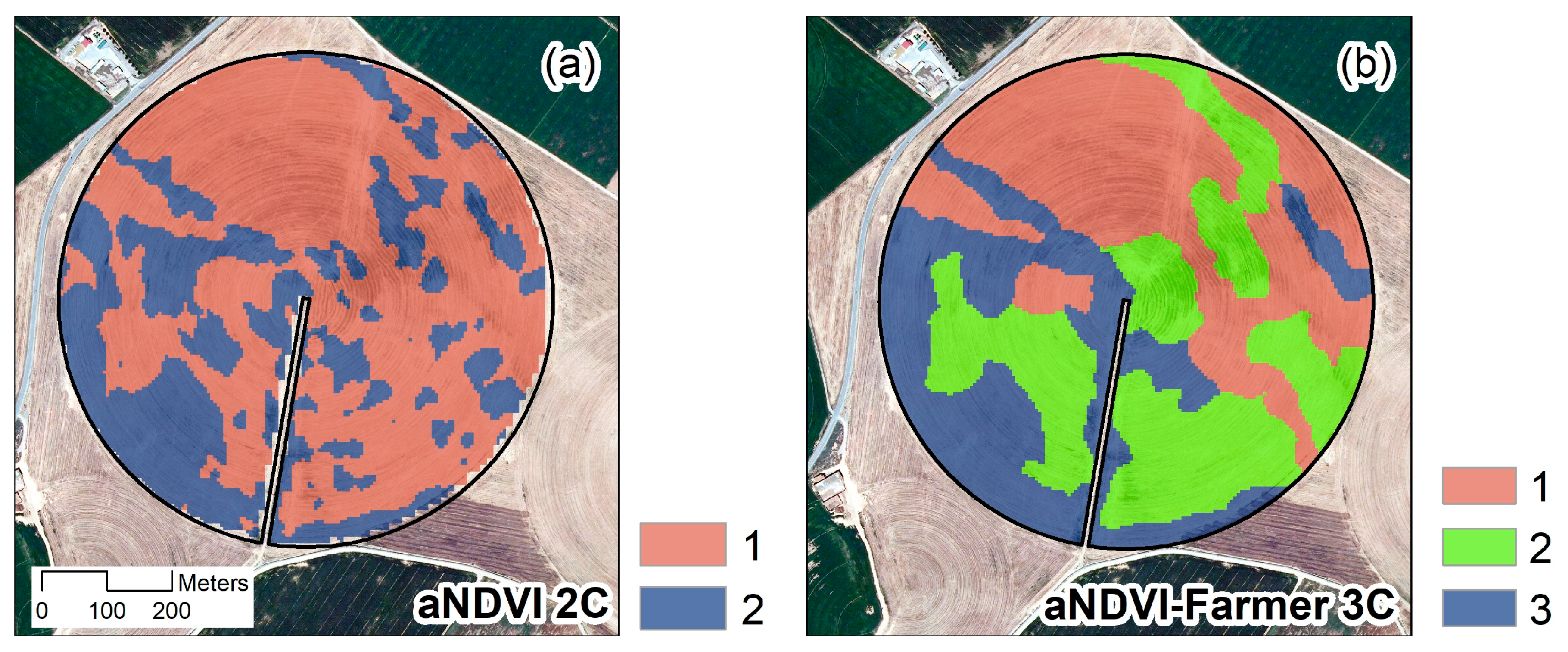
The farmer’s inertia to changes is usually slow and it is difficult for them to adopt new farming practices [
46]. However, we believe that their participation in the process of delineation of PMZs is important. In the present work, this contribution has been able to use the resulting areas of the unsupervised classification and segment them in such a way that an intermediate class of productive potential was added. This was in line with the idea of the farmer of avoiding high fragmentation. In addition, the results showed that the resulting three classes had statistically different average yields.


