Article

Studying Crop Yield Response to Supplemental Irrigation and the Spatial Heterogeneity of Soil Physical Attributes in a Humid Region

1
Department of Environmental Sciences, University of California, Riverside, 900 University Avenue, Riverside, CA 92521, USA
2
Department of Biosystems Engineering & Soil Science, University of Tennessee, 2506 E.J. Chapman Drive, Knoxville, TN 37996-4531, USA
3
Department of Agriculture, Nutrition, and Veterinary Science (ANVS), University of Nevada, Reno, Mail Stop 202, Reno, NV 89557, USA
*
Author to whom correspondence should be addressed.
Agriculture 2019, 9(2), 43; https://doi.org/10.3390/agriculture9020043
Submission received: 21 January 2019 / Revised: 20 February 2019 / Accepted: 20 February 2019 / Published: 23 February 2019
(This article belongs to the Special Issue Agricultural Irrigation)

Abstract

:
West Tennessee’s supplemental irrigation management at a field level is profoundly affected by the spatial heterogeneity of soil moisture and the temporal variability of weather. The introduction of precision farming techniques has enabled farmers to collect site-specific data that provide valuable quantitative information for effective irrigation management. Consequently, a two-year on-farm irrigation experiment in a 73 ha cotton field in west Tennessee was conducted and a variety of farming data were collected to understand the relationship between crop yields, the spatial heterogeneity of soil water content, and supplemental irrigation management. The soil water content showed higher correlations with soil textural information including sand (r = −0.9), silt (r = 0.85), and clay (r = 0.83) than with soil bulk density (r = −0.27). Spatial statistical analysis of the collected soil samples (i.e., 400 samples: 100 locations at four depths from 0–1 m) showed that soil texture and soil water content had clustered patterns within different depths, but BD mostly had random patterns. ECa maps tended to follow the same general spatial patterns as those for soil texture and water content. Overall, supplemental irrigation improved the cotton lint yield in comparison to rainfed throughout the two-year irrigation study, while the yield response to supplemental irrigation differed across the soil types. The yield increase due to irrigation was more pronounced for coarse-textured soils, while a yield reduction was observed when higher irrigation water was applied to fine-textured soils. In addition, in-season rainfall patterns had a profound impact on yield and crop response to supplemental irrigation regimes. The spatial analysis of the multiyear yield data revealed a substantial similarity between yield and plant-available water patterns. Consequently, variable rate irrigation guided with farming data seems to be the ideal management strategy to address field level spatial variability in plant-available water, as well as temporal variability in in-season rainfall patterns.

1. Introduction

1.1. Supplemental Irrigation Management in Humid Regions

Irrigated agriculture has been playing a globally significant role in providing roughly one-third of the total food and fiber supply [1]. While irrigated acreage is shrinking in some arid regions in the US due to increasing competition for water, supplemental irrigation is expanding in humid regions as a means to avoid unpredicted periods of water stress and maintain high yields [2]. For example, in west Tennessee, row crop irrigation has expanded rapidly from twenty-five center pivot irrigation systems installed in 2007 to 270 systems installed in 2012. This represents an expansion of 16,000 ha of cropland per year under supplemental irrigation [3], which necessitates an essential demand to study supplemental irrigation management of different crops in this region.
Precipitation is the main source of moisture in west Tennessee. However, severe in-season drought conditions for short periods are likely to occur, which could substantially reduce yields under rainfed agricultural practices. Supplemental irrigation is an irrigation strategy that attempts to maintain maximum yield production by irrigating during periods of insufficient rainfall to fulfill the crop water requirements. The application of supplemental irrigation management is a complex problem in west Tennessee, where precipitation patterns are temporally variable within and across cropping seasons and interact with the spatial mosaic of the physical and hydrological attributes of alluvial and windblown loess deposited soils. Soil properties, such as texture and bulk density, greatly affect soil water retention and movement and govern readily available soil water for crop irrigation management. Excess water content within the root zone could occur if irrigation adds to unpredicted rainfall events. This may cause insufficient aeration and consequent yield reduction. Moreover, runoff and deep percolation may lead to accelerated nutrient loss and soil erosion that in turn, increases the risk of contamination of nearby surface and/or groundwater.
Crop yield has been proven to be strongly related to soil physical properties. For example, Ref. [4] considered plant-available water (PAW: volumetric water content between the field capacity and the permanent wilting point within the root zone) as an input predictor of the wheat yield. They reported PAW as one of the dominant factors governing the spatiotemporal variation of yields. Soil texture was discussed by [5] as one of the greatest factors affecting the cotton yield. They found a relatively stable spatial pattern of yield over time, although yield and soil properties had stronger relationships during dry seasons than wet seasons. Graveel et al. [6] studied the response of corn to variations in soil erosion and sandy and silt textured profiles in west Tennessee and found a substantial difference in yield.
Cotton is a major crop in west Tennessee that is grown in more than 15 states and is vital to the US economy because it is a critical export-oriented product [7]. Currently, some 40% of US cotton is under irrigation, with the area expanding throughout the mid to southern US. Given the limited water resources in many cotton-growing areas, a considerable amount of research has recently been performed on cotton irrigation to improve the water use efficiency [8]. However, inconsistent cotton yields have been observed in response to irrigation in the humid portion of the US [9]. Suleiman et al. [10] studied the use of cotton deficit irrigation in a humid climate using FAO’s 56-crop coefficient method in Georgia and suggested establishing a 90 % irrigation threshold for the full irrigation of cotton in humid climates. Bajwa and Vories [11] evaluated the cotton canopy response to irrigation in a moderately humid area in Arkansas and found that under wet conditions, excessive irrigation decreased the yield of cotton lint. A similar result was reported by [12], who also found that excessive rainfall limited the yields from irrigation. Gwathmey et al. [13] conducted a four-year supplemental irrigation study in Jackson, Tennessee, and found a 38% improvement in lint yields at a 2.54 cm wk−1 supplemental irrigation rate compared to three of four years of the rainfed irrigation scenario. Grant et al. [14] used a surface drip irrigation system to investigate the response of the cotton yield to irrigation across different soil types with different PAW. This study illustrated that uniform irrigation is not the optimum management decision for the cotton wherever field-level soil heterogeneity affects the spatial distribution of PAW.

1.2. Farming Data and Precision Agriculture

Traditionally, irrigation studies were limited to small plots at research stations, mostly due to economic and computational limitations. Additionally, contemporary constraints to irrigation studies include the personnel time and expense for data collection, as well as the limitations of conventional computing infrastructure and statistical methods to analyze the increasingly larger spatiotemporal datasets that have inherent noise and uncertainty. In west Tennessee, the inherent heterogeneity and the spatiotemporal changes in soil and weather-related attributes of the region make it hard to extrapolate the results of design-based experiments on small plots to real field conditions. Supplemental irrigation scheduling is a site-specific irrigation management question where each field has its own irrigation management challenge that requires unique solutions. On-farm experimentation is an alternative for design-based experiments, since collecting site-specific information is becoming more and more common and affordable in US agriculture.
In contemporary agriculture, precision farming enables farmers to locally collect various site-specific information, such as the yield and soil apparent electrical conductivity (ECa). Crop yield maps provide valuable quantitative information on crop production, change in production, and the response of crop production to different agricultural inputs, including irrigation and fertilizer. Soil survey maps; soil sampling; on-the-go sensors; and remote sensing from field, airborne, and satellite sensors are the most widely used methods to obtain information on the spatial distribution of different soil attributes [15]. Soil sampling at the field-level provides valuable information on the spatial variation of soil attributes, but collecting this data has become laborious and expensive. ECa is a proxy for less accessible soil attributes, including soil texture and soil available water [16], and thus has created substantial interest in its use for soil mapping and management zone delineation in precision agriculture. ECa is measured in a simple and inexpensive way, where an electrical current is induced into the soil while the field is traversed. However, there are some inconsistencies in the literature concerning factors that affect the variability of ECa in non-saline fields [17]. This suggests the need to investigate the practical utility of using ECa for site-specific management in different regions, particularly because most of the supporting ancillary datasets including topographic edaphic features (e.g., elevation, slope, and aspect) are freely available. If not, these site-specific attributes can be measured and mapped without spending a considerable amount of time and money. Recently, new wireless technologies have enabled progressive farmers to remotely and continuously monitor soil properties over time, including soil temperature, soil water content, and soil matric potential.
Consequently, this study was carried out to understand the relationship between the spatial heterogeneity of soil and crop yields to better inform the management of site-specific supplemental irrigation in west Tennessee. The objectives of this study were to conduct an on-farm experiment and analyze yield maps to:
  • Assess the impact of the spatial heterogeneity of soil water content on the pattern of yield using on-farm data that was collected by the farmer’s soil moisture sensors and yield monitor systems;
  • Compare the cotton lint yield under different supplemental irrigation regimes across different soil types;
  • Assess the temporal stability of low/high yield zones by combining the measured historical yield data of different crops with available cotton yield data.

2. Materials and Methods
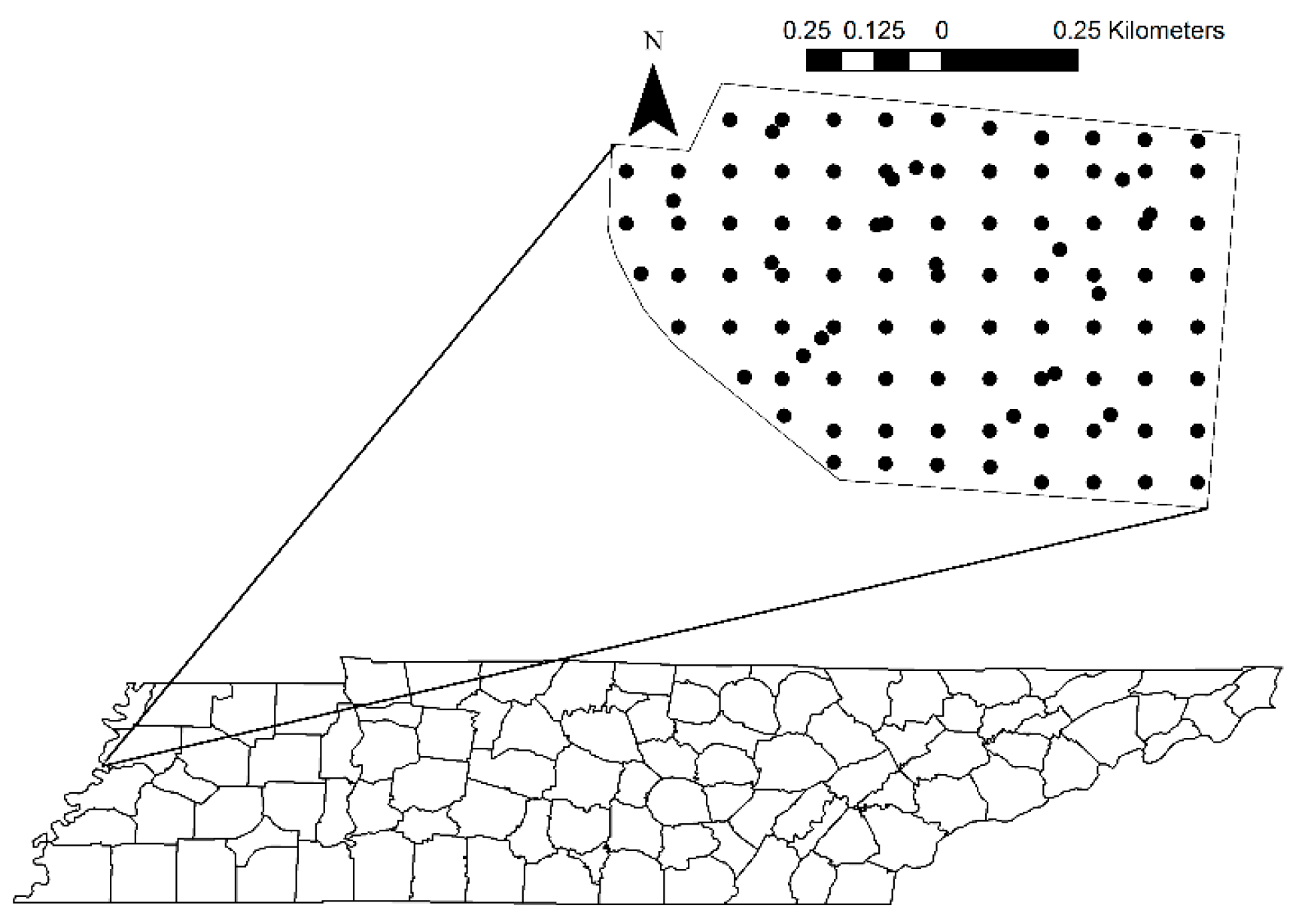
2.1. Study Area

The study area was a 73 ha irrigated field that is located in southwestern Dyer County in west Tennessee along the Mississippi river (Figure 1). The field was equipped with two center pivot irrigation systems that were used for the irrigation of no-till cotton during each cropping season. The field is on Mississippi river terrace alluvial deposits from which Robinsonville loam and fine sandy loam, Commerce silty clay loam, and Crevasse sandy loam soils have been produced (Figure 1). Figure 2 illustrates the long-term variability in regional climate. The mean monthly growing season precipitation and temperature is 97-mm month−1 and 21 °C from May to November, respectively (Figure 2). Rainfall is relatively high, even in dry years. Temperature changes are less pronounced and to some extent, inversely proportional to rainfall. The supplemental irrigation strategy has been growing in this region since rainfall events are not usually temporally well-scattered to fulfill the crop water requirement over the entire growing season.

2.2. Soil Data Collection and Lab Analysis

Haghverdi et al. [18] described the soil data collection where one hundred undisturbed samples (100 cm deep) were collected by a truck-mounted soil sampler between 21 and 22 March 2014 (Figure 1). Some 86 of these samples were collected using a grid sampling scheme where samples were about 100-m apart (i.e., half the mean semivariogram range of proxies). The rest of the samples (=14) were randomly collected from underneath the center pivot circles. The field sampling occurred after rainfall events, when the soil water status was assumed to be close to the field capacity.
Each 67-mm diameter core was sub-sampled at four depths between 0–100 cm in 25-cm increments, i.e., 0–25 cm, 25–50 cm, 50–75 cm, and 75–100 cm, with adjustments in respect to the available horizons. The mean depth across samples approximated 25 cm for all the layers. Hereafter, the word “layer” is used to describe subsamples rather than real soil horizons. The soil texture of each depth was estimated in the laboratory using a hydrometer [19]. The soil water content was estimated by subtracting oven-dried weights from wet weights. Bulk density (BD) was estimated as the oven dry weight to volume of each subsample. ECa was collected using a Veris 3100 (Veris Technologies, Salina, KS, USA) instrument on March 20, 2014 with 10 m and 20 m spacing between points in the same row and adjacent rows, respectively. The Veris 3100 has six rolling coulters for electrodes and collects two simultaneous ECa measurements from shallow (~0–30 cm) and deep depths (~0–90 cm).

2.3. Descriptive and Spatial Analysis of Soil Properties

The correlation between the volumetric water content at the time of sampling and soil texture, i.e., sand, silt, and clay percentages, and bulk density was investigated. A soil texture triangle was plotted for each of the four depths, with each depth layer being approximately 25-cm thick. The relationship between ECa data and soil physical information, obtained from soil samples, was studied. To match ECa and soil basic data, the ECa data were interpolated to each sample using an ordinary kriging approach [20].
The spatial analysis was done using ARCGIS 10.2.2 [21]. To examine the spatial autocorrelation of the attributes, the semivariogram (Equation (1)) and Global Moran’s I statistic (Equation (2), [22]) were obtained as follows:
γ ( h ) = 1 2 N ( h ) { i = 1 N ( h ) [ Z ( x i + h ) Z ( x i ) ] 2 }
where γ(h) is the semivariance; h is the interval class; N(h) is the number of pairs separated by the lag distance; and Z ( x i ) and Z ( x i + h ) are measured attributes at spatial location i and i + h, respectively. The nugget effect, sill, and range are the basic parameters of a semivariogram to describe the spatial structure. The nugget effect mostly represents sampling/measurement errors and variation at scales smaller than the sampling interval. The total variance is called the sill and the range is the maximum distance at which variables are spatially dependent.
The Global Moran’s I statistic is calculated as:
I = n i = 1 n j = 1 n w i , j × i = 1 n j = 1 n w i , j z i z j i = 1 n z i 2
where z is the deviation of an attribute from its mean, wi,j is the spatial weight between the ith and jth point, and n is equal to the number of points. Moran’s I is used to measure the degree of spatial autocorrelation or trend based on both feature locations and feature values simultaneously. Given a set of features and an associated attribute, it evaluates whether the pattern expressed is clustered, dispersed, or random [22]. The null hypothesis of this analysis states that the attribute being analyzed is randomly distributed among the features in the study area. Ordinary kriging was applied to samples of the ECa to generate maps that were compared and assessed against each other. A higher positive Moran’s Index for an attribute indicates a stronger spatial structure. The z-score changes in line with the Moran’s Index. A z-score from −1.65 to 1.65 shows that the spatial pattern is not significantly different than a random one. A z-score less than −1.65 is an indicator of a dispersed process, while a z-score greater than 1.65 displays a spatially clustered attribute.

2.4. On-Farm Irrigation Experiment

There were two center pivot systems available for irrigation within the 73-ha field. The on-farm experiment was conducted for two years and designed to study the supplemental irrigation-cotton lint yield relationship across different soil types. The farmer used a no-tillage method to plant ‘PHY375’ cotton variety on 30 May 2013 and ‘Stoneville 4946’ on 5 May 2014. The farmer used soil test recommendations for applications of variable rate potassium (K) and phosphorus (P). However, nitrogen was applied uniformly. Crop pest management was implemented following state extension recommendations and the field was harvested on 2 and 3 December 2013 and in the second year on 18–20 October 2014.
Throughout the experiment, we used the Management of Irrigation Systems in Tennessee (MOIST) program (http://www.utcrops.com/irrigation/irr_mgmt_moist_intro.htm) to discuss the efficiency of irrigation management with the farmer. MOIST is an irrigation decision support tool that delivers irrigation recommendations by simultaneously measuring and monitoring soil water status and calculating water balance through a deployed wireless soil sensor network. An on-farm weather and soil monitoring station contained a number of METER Devices (METER Group, Inc., Pullman, WA, USA), including an EM50G remote data logger, a VP-3 temperature and relative humidity sensor, an ECRN-100 high-resolution rain gauge, and a pyranometer: a solar radiation sensor, was installed in 2013 and run through 2014 using the MOIST program. Three additional stations with rain gauges and soil moisture sensors were added in 2014. Each station also had two MPS-2 soil matric potential and temperature sensors (METER Group, Inc., Pullman, WA, USA) installed at approximately 10 and 46 cm depths to monitor the soil water status. MOIST calculates the daily reference evapotranspiration (ETref) using Turc’s 1961 equation (developed for regions with relative humidity > 50%, [23]) as follows [24]:
E T r e f = 0.013 × ( T T + 15 ) × ( R s + 50 )
where ETref is the daily reference evapotranspiration (mm d−1), Rs is the daily solar radiation (Cal cm−2 d−1), and T is the daily mean air temperature (°C). The data for each station were recorded once per hour, stored in the logger, and then transmitted to a web-based interface. The farmer managed irrigation applications. At the same time, we wanted to make sure that he was provided with sufficient information to irrigate appropriately, while maintaining statistical variability of the supplemental irrigation water applied (IW) across the field to fulfill our research purpose. In 2014, we started sending out weekly MOIST reports to the farmer. The report contained information on the soil water status and irrigation scheduling based on soil sensors and water balance calculations.
Two different methods were used to create irrigation application zones across the field: programming the two pivots (pie shape zones) and partially swapping the sprinkler nozzles (arc shape zones). Table 1 summarizes the information on the irrigation programs at each pivot. The farmer’s routine irrigation schedule was 15.50 mm and 9.91 mm per revolution for the east and west pivots, respectively. The east (west) pivot panel was programmed to apply ±5.08 (±1.78) mm variation in irrigation per revolution on some pie shape zones. The control panels of pivots were Valley Select2 (Valmont Industries, Inc.) that were programmable for up to nine different pie shape zones. The program changes the irrigation rate by adjusting the pivot’s travel speed, where speeding up the pivot causes less irrigation and slowing it down applies additional irrigation. Based on the pivots’ characteristics and soil spatial variation, multiple banks of sprinklers were also selected and re-nozzled to form arc-shape irrigation zones. The center pivots can be operated both clockwise and counterclockwise, but were programmed only in the clockwise direction (Table 1).
We installed three Agspy (AquaSpy Inc., San Diego, CA, USA) soil moisture probes at three randomly selected points each year to monitor the soil water status, across pie-shape zones throughout the irrigation seasons. The AgSpy soil moisture capacitance probes were 1-m in length and obtained measurements at 10 depths at 0 to 100 cm, with 10 cm increments. The sensor output is a dimensionless number in the range 0 to 100, called the scaled frequency (SF), which is defined as:
S F = ( F a F s ) ( F a F w ) × 100
where Fa is the frequency of oscillation in air (air count), Fs is the frequency of oscillation in soil (soil count), and Fw is the frequency of oscillation in water (water count). The Fa and Fw are calculated during the manufacturing of each sensor. The frequency of oscillation is related to the capacitance between sensor plates that is in turn influenced by the relative permittivity of the soil media. The relative permittivity of water is significantly greater than that of air and soil, thereby changes in soil water content will be detected by the sensor [25].
Table 2 summarizes irrigation and weather data for the 2013 and 2014 cropping seasons. The sensors were installed a couple of weeks after planting and were removed prior to the harvest period. Consequently, in situ data were not available for the whole cropping seasons. However, temperature and precipitation data from the closest weather station were obtained from the National Climate Data Center [26] to fill these gaps.

2.5. Multiyear Yield Data Analysis

To better understand the spatiotemporal dynamics of changes in yield, several years with different crops should also be considered [27]. Except for 2011, yield data from 2007 to 2012 (i.e., corn 2007, corn 2008, soybean 2009, cotton 2010, cotton 2012) had been collected by the producer using appropriate yield-monitor-equipped harvesters (Table 3). We combined these data with the 2013 and 2014 yield data to analyze the relative difference and temporal variance of yield on the study site under both rainfed and supplemental irrigation.
A multistep filtering process was designed and implemented in Microsoft Excel and ArcGIS 10.2.2 [21] to process the yield data and produce final yield maps. First, the yield maps were visually assessed using the farmer’s knowledge of field conditions to identify potential unexpected patterns. Second, the data were color-coded based on harvest time to investigate the GPS tracks and movement of the harvester. Then, multiple filters were designed (e.g., using swath width, distance, speed of the harvester, change in speed) to remove outliers and erroneous data points. Last, yield data that were >±3 standard deviations of the mean were assumed to be outliers and removed from the analysis. Then, the field was divided into 100 m2 cells, and relative yield difference (Equation (5)) and yield temporal variance (Equation (6)) across years were calculated as follows [28]:
y ¯ i = 1 n k = 1 n [ y i , k y ¯ k y ¯ k ] × 100
where n is the number of years with yield data available, y ¯ i is the average percentage yield difference at cell i, y ¯ k is the average yield (Mg ha−1) across cells at year k, and y i , k is the yield value (Mg ha−1) at cell i at year k.
σ ¯ i 2 = 1 n k = 1 n ( y i , k y ¯ i , n ) 2
where σ ¯ i 2 is the temporal variance at cell i, y ¯ i , n is the average yield across the n years, and other variables are as previously defined.

3. Results and Discussion

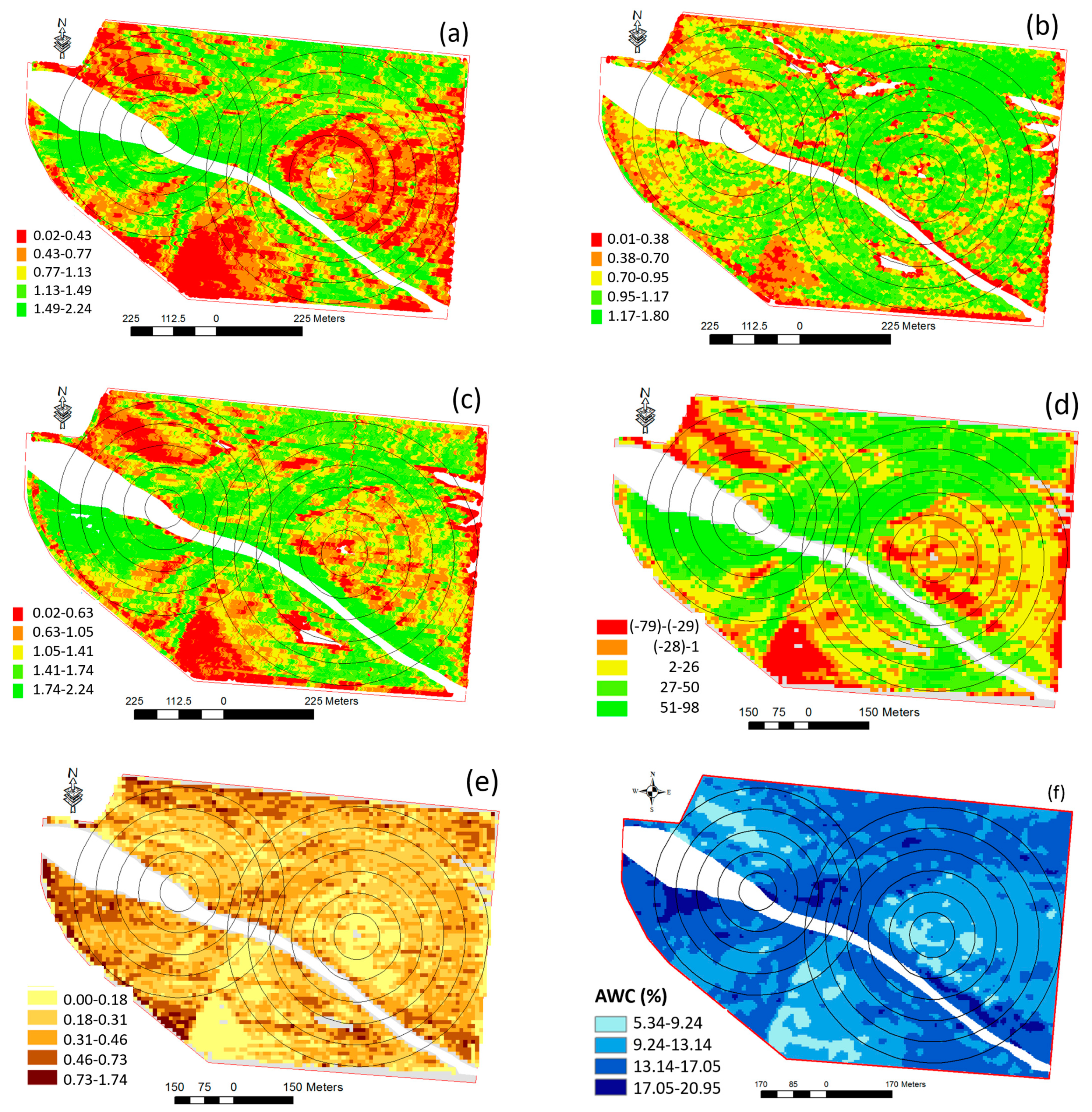
3.1. Field-Level Soil Heterogeneity and Application of Soil ECa

Table 4 contains descriptive statistics for the measured soil properties. The BD had its highest mean value at the deepest layer, while the mean value was almost identical among other layers. The mean water content decreased with depth, while its standard deviation slightly increased. The higher water content in the surface layer is likely attributed to textural differences among layers and also rainfall events prior to the sampling, which built the moisture level up within the top layers, but perhaps did not fully penetrate to the deeper layers. The mean sand percentage increased with depth, which was inversely proportional to a decline in silt and clay. The mean and standard deviation of the deep ECa readings (27.52 ± 18.73) were greater than those of shallow readings (24.64 ± 10.66). The standard deviation among deep ECa reading was almost twice that of shallow readings. The same result was reported by [29] on differences between the standard deviation and distribution of shallow versus deep ECa readings.
The soil texture drastically varied across the field such that almost the entire soil texture triangle was covered by the collected samples, except for the silt and clay textures (Figure 3). There was a shift from fine to coarse textures by depth, with sand showing the greatest particle increase. The sand had the highest absolute correlation with the soil moisture of the samples, while there was a weak negative correlation between BD and the water content (Figure 4), showing that soil texture was the dominant attribute governing water content. There was a clear pattern in clay and silt percentage plots versus water content; the majority of the samples with lower clay and silt contents belonged to the deeper layers (a cluster of black dots in the soil texture triangle), while samples from the shallower layers were more likely to have higher clay and silt contents. The opposite was seen in the sand versus water content plot.
Table 5 presents the semivariogram and Global Moran’s Index parameters for the selected attributes for each soil layer. The highest range did not belong to the same layer across soil properties. The average range varied from 200 m to 300 m among attributes, which was two to three times greater than the sampling intervals. The percent of nugget ranged from 18 to 50% among soil properties in the study of [30], who investigated the spatial variability of soil physical properties of alluvial soils in a 162 ha cotton field in Mississippi. This was somewhat similar to what was found for all the attributes except BD, which reached a nugget percent as high as 73 percent. The z-scores revealed all the attributes except BD within different layers had clustered patterns. BD only showed a clustered pattern at the third layer and had a random pattern at other layers.
Figure 5 shows maps interpolated by ordinary kriging. The white strip expanding from the northwest to southeast of the field is a surface drainage pathway. There are three major sandy regions within the field of study at the surface layer located at: (i) surrounding pivot points at the eastern part of the field; (ii) south of the field, mostly outside of the irrigated zones; and (iii) northwest part of the field. The sequence of sand maps from the first to fourth layers illustrate how these coarse soil regions expanded across the field by depth such that sand covered the majority of the field in deeper layers. The sandy regions could be either river flood-induced sand boils or earthquake-induced sand blows. The vertical arrangement of soil textural components was not consistent across the field. The clay had its highest influence from 0–50 cm, yet sand was the dominant particle from 50–100 cm. The observed depth to sand during sampling ranged from 15–75 cm across the field, with an average depth of 40 cm for almost 40% of the sampling spots. For the rest of the samples (60%), either there was no clear immediate change from fine texture to coarse texture or sand appeared at the surface soil. The silt contributed highly in subsurface layers (25–75 cm), where it reached its highest quantity and SD (Table 4). The majority of the samples from subsurface layers (50–75 cm) with a high silt content were compacted to some extent. This compaction was also projected in relatively higher BD values from the same layers (Table 4). The BD map of the third layer corresponded well to the textural patterns, where higher BD matched coarse samples. However, it was difficult to identify a trend from the rest of the BD maps, as was expected from the results of the spatial analysis (Table 5).
The soil water content is a dynamic property of soil with time. However, it is expected that a one-time measurement of water content values across a field provides a useful insight into the relative spatial pattern of soil hydraulic properties [31]. The water content map of the surface soil clearly showed the sandy textured areas as regions with a lower water content (Figure 5). At deeper depths, the water content maps almost exactly matched the spatial pattern of the sand maps. This occurred because coarse soils tend to dry out faster and hold less water than finer textured soils. This suggests that a one-time measurement of water content during the sampling process may be mathematically transformable to a PAW map. Overall, the water content map for the entire profile (0–100 cm) was similar to maps of individual layers.
The ECa maps tended to follow the same general spatial patterns as those for soil basic properties and water content (Figure 5). Table 6 illustrates the correlation coefficient between ECa values and soil basic data. The ECa data were moderately correlated to soil texture and water content information. The lowest correlation was between BD and ECa data. The correlation between shallow ECa and other attributes declined from layer 1 to 4, as expected, while the opposite was true for ECa deep readings. Sudduth et al. [29] showed that 90% of the shallow and deep reading responses in Veris machines were approximately obtained from the soil above the 30 cm and 100 cm depths, respectively. The sand increased with depth, hence regions with high conductivity became less pronounced in the deep ECa map as opposed to the shallow ECa map.
This study demonstrated that ECa is a useful surrogate for both soil texture and water content. Sudduth et al. [29] studied ECa readings on 12 fields in six states of the north-central US. They found a good relationship between ECa data and soil cation exchange capacity (CEC), as well as clay content at different times and locations, thus suggesting a general calibration equation of CEC and clay content to ECa readings. They found the most variation in ECa values in Iowa fields that had the widest range in soil texture, from loam to clay loam. In contrast, [17] reported water content as the main factor influencing ECa readings in a rainfed field, but they did not find soil texture to be a significant predictor of ECa. They found a weak correlation between water content and clay content and found that other factors including elevation and organic matter, may govern the amount of soil water content [17]. In theory, multiple factors, including the relative fractions occupied by soil, water and air, geometry and distribution of particles, and soil solution attributes, affect ECa [32]. The current introduced to measure the ECa of soil, in fact, travels through liquid, soil-liquid, and solid pathways [33]. We believe an accurate understanding of field-level soil texture variability and soil water status during the ECa measurement process is crucial to efficiently interpret ECa maps. Brevik et al. [34] studied the temporal stability of ECa data with respect to soil water content. They observed a strong influence of water content on ECa readings and found that ECa’s power to differentiate soils was proportional to soil moisture. They mentioned that soil water content should be reported as an essential part of ECa studies. In this study site, the spatial heterogeneity of soil texture was the main factor that governed the spatial distribution of water content. Further studies, however, are needed to examine the efficacy of ECa for other typical field-level heterogeneity in the region, where the infiltration and redistribution of water within the root zone is governed by topography rather than soil textural variability.

3.2. Cotton Supplemental Irrigation

Table 7 summarizes the correlation coefficients between yield data and some soil properties across the field of study. To evaluate the effect of variable rate fertilizer application by the farmer on yield spatial variation, we also obtained correlation information for P and K. In general, correlation coefficients were higher for 2014 data than for 2013 data. The correlations between P and K with yield data were negligible. Given the high correlation between ECa data and PAW [18], the ECa data were used to group cotton lint yield information into four soil-based zones (Figure 6). The results illustrated in Figure 6 include irrigated areas, as well as corners of the field that were rainfed. In general, there was an increase in yield from soils with lower ECa to soils with higher ECa in 2014, but not in 2013. This is in line with the relatively higher correlation between water content/soil texture and the yield data in 2014 compared to 2013.
In 2013, only for coarse-textured soils (soils with lower ECa readings; zones 1 and 2), there was an overall positive response to supplemental irrigation. We observed no consistent positive response to higher irrigation levels for soils with higher ECa readings (i.e., zone 3 and 4 repressing fine-textured soil with higher PAW). In 2014, overall, cotton responded favorably to higher supplemental irrigation levels for the first three ECa zones, with coarse-textured soil showing the highest yield increase. The highest yield for the fine-textured zone (zone 4) did not belong to the greatest irrigation applications.
Figure 7 and Figure 8 depict the dynamic of soil moisture (Agspy sensors) at different depths and locations over the 2013 and 2014 growing seasons, respectively. There were some missing data and bad readings mostly in 2014. In 2013, soil moisture probes a, b, and c were located underneath the east pivot, representing the pie shape zone with extra irrigation, pie shape zone with lower irrigation, and farmer’s irrigation application, respectively. The soil moisture probes a, b, and c received 163 mm, 90 mm, and 133 mm seasonal IW, respectively. The average predicted PAW throughout the effective root zone (i.e., 1 m) was 0.28 m3 m−3, 0.22 m3 m−3, and 0.30 m3 m−3 for probes a, b, and c, respectively [18]. The pattern of soil moisture was dynamic and varied among sensors at different locations and depths. At probe a, soil moisture depletion and replenishment occurred for sensors up to 40 cm deep during the monitoring period (i.e., days after planting (DAP): 42-133). Soil water status remained almost unchanged for deeper sensors for about 100 DAP, and then gradually exhibited a reduction, indicating that roots started to pull out water from deeper layers as the ET demand increased. At probe b, rainfall plus irrigation kept the soil moisture at a fairly constant level up to about 80 DAP for all sensors, while fluctuations decreased by depth, as expected. After that, there was a substantial depletion in soil moisture for sensors up to 50 cm, which even expanded to deeper sensors at about 95 DAP. At probe c, the overall trend was similar to that of probe a. Toward the end of the growing season, much rainfall at 112 DAP occurred that refilled the shallow layers for all soil moisture probes and also penetrated to deeper layers such that there was an increase in readings by the soil moisture sensors at 30 and 40 cm and no decrease for deeper sensors up to the end of the monitoring period.
In 2014, soil moisture probes a, b, and c were mainly located underneath the west pivot, representing the central area irrigated by both pivots, pie shape zone with lower irrigation, and farmer’s irrigation application, respectively. Soil moisture probes a, b, and c (Figure 8) received 142, 42, and 50 mm of IW, respectively, during the 2014 cropping season. Within the effective root zone (i.e., 1m), the average PAW values predicted for probes a, b, and c were 0.19 m3 m−3, 0.33 m3 m−3, and 0.23 m3 m−3, respectively [18]. Unlike 2013, most of the deeper sensors in 2014 showed some fluctuations starting at about 70 DAP, meaning that the crop started to use water from deeper layers as the crop water requirement increased. We attribute this to (i) bigger plants with larger canopies, and hence a higher ET demand; (ii) lower irrigation in 2014 compared to 2013; and (iii) lower irrigation under the west pivot (where we had sensors installed in 2014) compared to the east pivot (where we had sensors installed in 2013). Trends in probes b and c were similar. There were more fluctuations in the shallow sensors in probe a, since this sensor was irrigated by both pivots and was located on a coarse-textured soil with a low PAW. In both years, heavy rainfall events were responsible for big changes in the soil water status within the soil profile and considering sensor fluctuations, they usually penetrated deep down to 50 cm. Irrigation events, however, mostly refilled shallow layers up to 20 cm and barley influenced sensors deeper than 30 cm.
The cotton lint response to supplemental irrigation differed across soil types. For soils with a lower PAW, there was a positive response to irrigation in comparison to rainfed, where soil moisture deficit is expected to reduce the boll number and yield [9]. The cotton response to irrigation was not consistent for soils with a higher PAW, except that a yield reduction occurred underneath both pivots for high irrigation rates in both cropping seasons. This is in line with the reported results in the literature, indicating that under wet conditions, excessive irrigation decreased the yield of cotton lint [11,12]. In 2013, the cotton lint yield was only 12% higher where we placed probe a (IW = 163 mm, predicted PAW = 0.28 m3 m−3) in comparison to the yield at probe b (IW = 90 mm, predicted PAW = 0.22 m3 m−3), even though there was a remarkable difference in soil water status throughout the growing season between the two soil moisture probes (Figure 7). On the other hand, in 2014, the yield difference between the exact same spots with a similar relative difference in IW increased by 44%. We attribute this to the wet season and delayed planting in 2013, which significantly affected the cotton response to irrigation. Delayed planting influences heat unit accumulation and distribution, which was underscored as an important factor for the short season cotton response to supplemental irrigation by [13]. Moreover, irrigation is expected to increase the number of bolls, but delays cutout (i.e., cessation of flowering) since irrigation continues the vegetative growth for a longer period. We believe that rapid canopy expansion occurred on soil with a higher PAW in 2013 due to excessive water within the crop effective root zone.
Both 2013 and 2014 were relatively wet years. In fact, the rainfall was always above the long term average, except for July 2014. There were some heavy rainfall events during the growing seasons, which caused a significant increase in the soil water content. This is a typical situation in west Tennessee, with unexpected rainfall events, where temporal changes in rainfall patterns significantly affect the yield response to supplemental irrigation across years. Bajwa and Vories [11] reported the same complexity on cotton irrigation scheduling in a moderately humid area in Arkansas when rainfall was plentiful and caused a yield reduction for high irrigated crops. Monitoring the soil water status revealed that rainfall events refilled the top soil and penetrated into deeper layers, while supplemental irrigation mostly influenced the shallow layer up to 20 cm. Therefore, any sustainable irrigation management in this region should take effective rainfall into account for site-specific irrigation scheduling. Sensors indicated fast depletion for soils with lower PAWs. This caused the crop to start using water from deeper layers as the cropping season advanced and ET demand increased. The sensor located on the overlap region of the two pivots showed that more frequent irrigation could prevent the shallow soil layer from substantial depletion and possible yield reduction due to water stress and thus should be considered as a potential irrigation strategy for coarse-textured soils with low PAWs throughout the study site. On the other hand, days with no rainfall and irrigation could be beneficial for soils with high PAWs since cotton usually responds favorably to periods of water stress adequate to reduce vegetation expansion. The farmer’s goal was to tailor irrigation decisions to dominant soil areas, while avoiding over and under irrigation as much as possible. The results, however, show that uniform irrigation management can be detrimental to the field’s overall production and water use efficiency. Consequently, variable rate irrigation strategies were predicted to enhance cotton production compared to current uniform irrigation management practiced by the grower [35]. There may be a requirement to practice a dynamic zoning strategy considering available water for the crop within its effective root zone during growing seasons [36]. Soil moisture data will be instrumental to making the most informed decisions for each soil and to determining how much different soils of a variable texture need to be irrigated to maximize production.

3.3. Multiyear Yield Analysis

Figure 9 illustrates the cotton yield maps for 2012, 2013, and 2014; mean yield map (from Equation (5)); and standard deviation yield map (from Equation (6)). We included the 2012 yield map, a year before this experiment when uniform irrigation had been applied by the farmer, to better represent the effect of soil spatial variation on the cotton yield. Thematic cotton yield maps for 2012 and 2014 cropping seasons followed the same spatial distribution as soil texture and water content maps, but the 2013 yield map showed a different pattern. This finding agrees with the low correlation observed between cotton yield data in 2013 and soil properties (Table 7). The spatial analysis of the multiyear mean yield map (ranged from −79 to 98) showed substantial similarity to the PAW map developed for the field of study by [18]. There were three regions with a lower yield and all on coarse-textured soils with lower PAW. The highest yield temporal stability also belonged to the regions with low PAW, (i) in the southern part of the field outside pivots coverage and (ii) in an area surrounding the east pivot point. The yield temporal stability was lower for other parts of the field, but it was hard to identify any cluster of cells with a similar temporal variance. We mainly attribute this to different rainfall patterns and irrigation regimes across years, and their effects on the yield across soil types, which caused substantial mean yield variability across years (Table 3). For instance, for cotton and corn, there was as much as 43% and 110% temporal differences between mean yields across years, respectively. However, it is known that other attributes related to management, water, crop, and climate affect the crop yield in a complex manner and the crop yield maps per se only provide limited information about the influence of each attribute [31]. In 2012 and 2014, the mean yield and standard deviation were higher than those for 2013, indicating a decline in yield on soils with higher available water in 2013 due to the delayed planting and excessive rainfall throughout the growing season.

4. Conclusions

Irrigation investment has been expanding across the humid areas of the US Cotton Belt for the last 20 years because of the stabilization of yields and high commodity prices. Recent advances in modern instrumentation and measurement techniques, such as on-the-go sensing, remote sensing, and wireless networks of sensors, make site-specific on-farm experimentation possible for farmers. This is essential for field-level cotton irrigation management in humid areas as a complex problem due to substantial spatiotemporal heterogeneity in soil and weather-related parameters. In this study, we used a variety of information that is relatively easily collected by farmers, to investigate the impact of the spatial and temporal heterogeneity of soil attributes, including field-collected soil texture, moisture, ECa, and bulk density, on the cotton response to supplemental irrigation. We found that ECa was a useful proximal attribute to understand field-level spatial variability of alluvial soils in the region. Analyzing crop yield against maps of soil characteristics revealed that soil texture and soil water content remarkably influenced yield patterns, suggesting that variable rate irrigation is the appropriate irrigation scenario for this mixture of soils. We also found that other factors, including cropping season length and in-season rainfall pattern, may change or even reverse the expected lint yield from an irrigation treatment for a specific soil type. While soil variation is inherent and not controlled by farmers, irrigation, if well-scheduled, could be the key factor to optimizing the crop production and water use efficiency. The use of soil moisture sensors can help monitor soil water status and adjust irrigation application based on in-season rainfall patterns and within-field soil variability.

Author Contributions

Conceptualization, A.H. and B.L.; methodology, A.H. and B.L.; software, A.H. and B.L.; validation, A.H. and B.L.; formal analysis, A.H.; investigation, A.H.; resources, B.L..; Data curation, A.H., B.L., W.C.W., S.G., T.G., M.Z., and P.V.; writing—original draft preparation, A.H.; writing—review and editing, A.H., B.L., R.W-A., and T.G.; visualization, A.H.; supervision, B.L.; funding acquisition, B.L.

Funding

This project was funded in part by Cotton Inc. and the United States Department of Agriculture (USDA) Natural Resources Conservation Service (NRCS) Conservation Innovation Grants (CIG).

Acknowledgments

We appreciate Pugh Brothers Farms for allowing us to implement this project on their property.

Conflicts of Interest

The authors declare no conflict of interest. The funders had no role in the design of the study; in the collection, analyses, or interpretation of data; in the writing of the manuscript, or in the decision to publish the results.

References

  1. FAO (Food and Agriculture Organization of the United Nations). Statistical Yearbook 2013: World Food and Agriculture; FAO: Rome, Italy, 2013. [Google Scholar]
  2. NASS (National Agricultural Statistics Service). 2007 Census of Agriculture: Farm and Ranch Irrigation Survey, National Agricultural Statistics Service, USDA. 2010. Available online: http://www.agcensus.usda.gov/index.php (accessed on 22 March 2019).
  3. Tennessee Farm Bureau Federation. Irrigation: Solving Potential Challenges: Policy Development 2013. 2013. Available online: https://www.tnfarmbureau.org/wp-content/uploads/2010/10/Irrigation.pdf (accessed on 22 March 2019).
  4. Wong, M.T.F.; Asseng, S. Determining the Causes of Spatial and Temporal Variability of Wheat Yields at Sub-field Scale Using a New Method of Upscaling a Crop Model. Plant Soil 2006, 283, 203–215. [Google Scholar] [CrossRef]
  5. Guo, W.; Maas, S.J.; Bronson, K.F. Relationship between cotton yield and soil electrical conductivity, topography, and Landsat imagery. Precis. Agric. 2012, 13, 678–692. [Google Scholar] [CrossRef]
  6. Graveel, J.G.; Fribourg, H.A.; Overton, J.R.; Bell, F.F.; Sanders, W.L. Response of Corn to Soil Variation in West Tennessee, 1957–1980. JPA 1989, 2, 300–305. [Google Scholar] [CrossRef]
  7. Perry, C.; Barns, E. Cotton Irrigation Management for Humid Regions; Cotton Inc.: Cary, NC, USA, 2012. [Google Scholar]
  8. Vellidis, G.; Liakos, V.; Perry, C.; Tucker, M.; Collins, G.; Snider, J.; Andreis, J.; Migliaccio, K.; Fraisse, C.; Morgan, K.; et al. A smartphone app for scheduling irrigation on cotton. In Proceedings of the 2014 Beltwide Cotton Conference, New Orleans, LA, USA, 6–8 January 2014; Boyd, S., Huffman, M., Robertson, B., Eds.; National Cotton Council: Memphis, TN, USA, 2014. [Google Scholar]
  9. Pettigrew, W.T. Moisture Deficit Effects on Cotton Lint Yield, Yield Components, and Boll Distribution. Agron. J. 2004, 96, 377. [Google Scholar] [CrossRef]
  10. Suleiman, A.A.; Soler, C.M.T.; Hoogenboom, G. Evaluation of FAO-56 crop coefficient procedures for deficit irrigation management of cotton in a humid climate. Agric. Water Manag. 2007, 91, 33–42. [Google Scholar] [CrossRef]
  11. Bajwa, S.G.; Vories, E.D. Spatial analysis of cotton (Gossypium hirsutum L.) canopy responses to irrigation in a moderately humid area. Irrig. Sci. 2007, 25, 429–441. [Google Scholar] [CrossRef]
  12. Bronson, K.F.; Booker, J.D.; Bordovsky, J.P.; Keeling, J.W.; Wheeler, T.A.; Boman, R.K.; Parajulee, M.N.; Segarra, E.; Nichols, R.L. Site-Specific Irrigation and Nitrogen Management for Cotton Production in the Southern High Plains. Agron. J. 2006, 98, 212. [Google Scholar] [CrossRef] [Green Version]
  13. Gwathmey, C.O.; Leib, B.G.; Main, C.L. Lint yield and crop maturity responses to irrigation in a short-season environment. J. Cotton Sci. 2011, 15, 1–10. [Google Scholar]
  14. Grant, T.J.; Leib, B.G.; Duncan, H.A.; Main, C.L.; Verbree, D.A. A deficit irrigation trial in differing soils used to evaluate cotton irrigation scheduling for the Mid-South. J. Cotton Sci. 2017, 21, 265–274. [Google Scholar]
  15. Khosla, R.; Westfall, D.G.; Reich, R.M.; Mahal, J.S.; Gangloff, W.J. Spatial Variation and Site-Specific Management Zones. In Geostatistical Applications for Precision Agriculture; Springer Nature: Berlin, Germany, 2010; pp. 195–219. [Google Scholar]
  16. Gooley, L.; Huang, J.; Page, D.; Triantafilis, J. Digital soil mapping of available water content using proximal and remotely sensed data. Soil Use Manag. 2013, 30, 139–151. [Google Scholar] [CrossRef]
  17. McCutcheon, M.C.; Farahani, H.J.; Stednick, J.D.; Buchleiter, G.W.; Green, T.R. Effect of Soil Water on Apparent Soil Electrical Conductivity and Texture Relationships in a Dryland Field. Biosyst. Eng. 2006, 94, 19–32. [Google Scholar] [CrossRef]
  18. Haghverdi, A.; Leib, B.G.; Washington-Allen, R.A.; Ayers, P.D.; Buschermohle, M.J. High-resolution prediction of soil available water content within the crop root zone. J. Hydrol. 2015, 530, 167–179. [Google Scholar] [CrossRef]
  19. Blake, G.R.; Hartge, K.H. Bulk density. In Methods of Soil Analysis. Part 1, 2nd ed.; Agron. Monogr. 9; Klute, A., Ed.; ASA and SSSA: Madison, WI, USA, 1986; pp. 363–375. [Google Scholar]
  20. Cressie, N. Spatial prediction and ordinary kriging. Math. Geol. 1988, 20, 405–421. [Google Scholar] [CrossRef]
  21. ESRI. ArcMap (Version 10.2.2); Environmental Systems Resource Institute: Redlands, CA, USA, 2014. [Google Scholar]
  22. Getis, A.; Ord, J.K. The Analysis of Spatial Association by Use of Distance Statistics. Geogr. Anal. 2010, 24, 189–206. [Google Scholar] [CrossRef] [Green Version]
  23. Turc, L. Estimation of irrigation water requirements, potential evapotranspiration: A simple climatic formula evolved up to date. Ann. Agron. 1961, 12, 13–14. [Google Scholar]
  24. Lu, J.; Sun, G.; McNulty, S.G.; Amatya, D.M. A comparison of six potential evapotranspiration methods for regional use in the southeastern United States. J. Am. Water Resour. Assoc. 2005, 41, 621–633. [Google Scholar] [CrossRef]
  25. Paterson, N.D.; Richard, J.C.; Neil, M.W. Soil Moisture Sensor with Data Transmitter. U.S. Patent 12/310,946, 10 December 2009. [Google Scholar]
  26. National Climate Data Center. National Climate Data Center Home Page. 2015. Available online: http://www.ncdc.noaa.gov/data-access/land-based-station-data (accessed on 13 June 2015).
  27. Joernsgaard, B.; Halmoe, S. Intra-field yield variation over crops and years. Eur. J. Agron. 2003, 19, 23–33. [Google Scholar] [CrossRef] [Green Version]
  28. Basso, B.; Bertocco, M.; Sartori, L.; Martin, E.C. Analyzing the effects of climate variability on spatial pattern of yield in a maize–wheat–soybean rotation. Eur. J. Agron. 2007, 26, 82–91. [Google Scholar] [CrossRef]
  29. Sudduth, K.; Kitchen, N.; Wiebold, W.; Batchelor, W.; Bollero, G.; Bullock, D.; Clay, D.; Palm, H.; Pierce, F.; Schuler, R.; et al. Relating apparent electrical conductivity to soil properties across the north-central USA. Comput. Electron. Agric. 2005, 46, 263–283. [Google Scholar] [CrossRef]
  30. Iqbal, J.; Thomasson, J.A.; Jenkins, J.N.; Owens, P.R.; Whisler, F.D. Spatial Variability Analysis of Soil Physical Properties of Alluvial Soils. Soil Sci. Soc. Am. J. 2005, 69, 1338. [Google Scholar] [CrossRef]
  31. Corwin, D.L.; Lesch, S.M.; Shouse, P.J.; Ayars, J.E.; Soppe, R.; Ayars, J.E. Identifying Soil Properties that Influence Cotton Yield Using Soil Sampling Directed by Apparent Soil Electrical Conductivity. Agron. J. 2003, 95, 352–364. [Google Scholar] [CrossRef]
  32. Friedman, S.P. Soil properties influencing apparent electrical conductivity: A review. Comput. Electron. Agric. 2005, 46, 45–70. [Google Scholar] [CrossRef]
  33. Rhoades, J.D.; Corwin, D.L.; Lesch, S.M. Geospatial measurements of soil electrical conductivity to assess soil salinity and diffuse salt loading from irrigation. In Solar Eruptions and Energetic Particles; American Geophysical Union (AGU): Washington, DC, USA, 1999; Volume 108, pp. 197–215. [Google Scholar]
  34. Brevik, E.C.; Fenton, T.E.; Lazari, A. Soil electrical conductivity as a function of soil water content and implications for soil mapping. Precis. Agric. 2006, 7, 393–404. [Google Scholar] [CrossRef]
  35. Haghverdi, A.; Leib, B.G.; Washington-Allen, R.A.; Buschermohle, M.J.; Ayers, P.D. Studying uniform and variable rate center pivot irrigation strategies with the aid of site-specific water production functions. Comput. Electron. Agric. 2016, 123, 327–340. [Google Scholar] [CrossRef] [Green Version]
  36. Haghverdi, A.; Leib, B.G.; Washington-Allen, R.A.; Ayers, P.D.; Buschermohle, M.J. Perspectives on delineating management zones for variable rate irrigation. Comput. Electron. Agric. 2015, 117, 154–167. [Google Scholar] [CrossRef]
Figure 1. The 73-ha supplemental irrigation study field is located in southwestern Dyer County in west Tennessee along the Mississippi river. Soil samples were collected at four depths from 0–1 meter at 100 locations.
Agriculture 09 00043 g001
Figure 2. The long-term climatic variation in rainfall (dashed line) and temperature (column) in west Tennessee. Temperature columns show the mean monthly minimum (in black) and the mean monthly maximum (in white).
Agriculture 09 00043 g002
Figure 3. The textural distribution of soil samples from four different depths between 0 to 1 meter, where the darker colors correspond to the deepest depths. The samples were collected from a 73-ha two-pivot irrigation field that is located in southwestern Dyer County, Tennessee.
Agriculture 09 00043 g003
Figure 4. The relationship of 400 samples at four depths from 0–1 meter of soil texture (% Clay, Silt, & Sand) and bulk density (BD) to volumetric water content from a 73-ha two-pivot field in west Tennessee. The light to darker colors of the data markers correspond to 0–1 meter depths.
Agriculture 09 00043 g004
Figure 5. Maps of six different soil properties and their range of variation within a 73-ha two-pivot field in west Tennessee. These attributes include percent silt, sand, and clay, bulk density (BD, g cm−3), volumetric water content (WC, %), and apparent electrical conductivity shallow (ECa-S, mS m−1) and deep (ECa-D, mS m−1). Numbers 1-4 denote layers 1–4 (layer 1: 0–25 cm, layer 2: 25–50 cm, layer 3: 50–75 cm, and layer 4: 75–100 cm). The maps were generated using ordinary kriging. The darker colors correspond to greater values for each attribute.
Agriculture 09 00043 g005
Figure 6. The effects of supplemental irrigation (blue bars, right-hand y-axis) on cotton lint yield (orange lines, left-hand y-axis) in 2013 and 2014 within a 73-ha two-pivot field in west Tennessee. The white and black five-point start symbols denote actual irrigation applications by the farmer for the west and east pivots, respectively. The deep ECa data were used to group cotton lint yield information into four zones, where ECa increases from zone 1 to zone 4, zone 1: 2–8 mS m−1, zone 2: 8–18 mS m−1, zone 3: 18–35 mS m−1, and zone 4: 35–162 mS m−1.
Agriculture 09 00043 g006
Figure 7. The change in soil moisture, measured as scale frequency (SF, Equation (4)), from 42 days after planting throughout the 2013 growing season in a 73-ha two-pivot supplemental irrigation field in west Tennessee. Light and dark blue bars show irrigation and rainfall, respectively. SF was measured using Agspy soil sensor probes at different locations and 10 depths from 0–1 m. In 2013, soil moisture probes a, b, and c were located underneath the east pivot, representing the pie shape zone with extra irrigation, pie shape zone with lower irrigation, and farmer’s irrigation application, respectively.
Agriculture 09 00043 g007
Figure 8. The change in soil moisture capacitance, measured as scale frequency (SF, Equation (4)), from 53 days after planting throughout the 2014 growing season in a 73-ha two-pivot supplemental irrigation field in west Tennessee. Light and dark blue bars show irrigation and rainfall, respectively. SF was measured using Agspy soil sensor probes at different locations and 10 depths from 0–1 m. In 2014, soil moisture probes a, b, and c were mainly located underneath the west pivot, representing the central area irrigated by both pivots, pie shape zone with lower irrigation, and farmer’s irrigation application, respectively.
Agriculture 09 00043 g008
Figure 9. The cotton lint yield map (Mg ha−1) time series from 2012 to 2014 (ac), plus mean ((d), using Equation (5)) and standard deviation cotton yield maps ((e), using Equation (6)) that were derived from the producer’s harvester data (Table 3, seven years of data for cotton, corn and soybean) for a 73-ha field in west Tennessee. The map of plant available water content (f) within the crop effective root zone (i.e., 100 cm) is adapted from the study by [18].
Agriculture 09 00043 g009
Table 1. Detailed information on the supplemental irrigation programs for the two center pivots within the 73-ha supplemental irrigation field that is located in southwestern Dyer County in west Tennessee for one revolution.
East PivotWest Pivot
Program SectorStart Angle 1
(degree)
Stop Angle
(degree)
Depth of Water
(mm)
Start Angle
(degree)
Stop Angle
(degree)
Depth of water
(mm)
19011010.412753159.91
2110015.4931533511.68
30 12020.573353558.38
4204010.413552359.91
5407015.4923525511.68
6709020.572552758.38
1 The zero degree was at north and pivots traveled clockwise.
Table 2. Growing season summary of weather and supplemental irrigation data in the 73-ha study area for the 2013 and 2014 growing seasons, in comparison to the 30-year mean for these variables. The study area is located in southwestern Dyer County in west Tennessee.
YearVariableMonth
MayJuneJulyAugustSeptemberOctoberNovember
2013Rain, mm23150190957911263
IW-East, mm 403162
IW-West, mm 152030
ETref 1, mm day−1 4.334.433.922.491.28
2014Rain, mm1431725612412018
IW-East, mm 6231
IW-West, mm 2030
ETref 1, mm day−14.154.424.864.513.472.94
30 yearRain, mm120101102748282117
Tmean, °C21252726221610
1 ETref: Reference evapotranspiration data that were calculated using the Turc equation (Equation (3)) from 19 July 2013 (7 May 2014) to 30 November 2013 (5 October 2014), IW: irrigation water applied by the farmer. The 30-year mean data collected from the closest weather station [26].
Table 3. Descriptive statistics on yield data (Mg ha−1) at the field of study located in southwestern Dyer County in west Tennessee.
YearCropMeanSD
2007Corn7.1374.158
2008Corn3.4200.903
2009Soybean3.2210.860
2010Cotton0.9470.306
2012Cotton0.9130.494
2013Cotton0.8710.329
2014Cotton1.2440.493
Table 4. Descriptive statistics for selected soil properties from different soil sampling layers. Soil samples were collected at four depths from 0–1 meter at 100 locations.
Variable 1LayerMin.Max.MeanSD
BD, g cm−31th1.121.661.360.10
2nd1.111.701.350.12
3rd1.061.861.340.12
4th1.171.781.400.13
total1.061.861.360.12
WC, %1th10.7559.7428.357.43
2nd7.2743.1226.0210.78
3rd5.9842.3821.6411.08
4th5.6745.3220.1811.15
total3.9447.6117.948.49
Sand, %1th8.7788.2538.0720.11
2nd0.0094.9846.3931.57
3rd2.5095.7061.3831.10
4th5.4696.8669.9026.09
Clay, %1th7.3747.5627.559.04
2nd2.5056.6022.1814.17
3rd1.2647.7214.2711.44
4th0.3437.1011.007.80
Silt, %1th4.3854.0634.3812.75
2nd0.0066.5131.4319.85
3rd0.0072.8124.3521.76
4th0.0069.2319.1019.83
ECa, mS m−1shallow1.6048.7024.6410.66
ECa, mS m−1deep1.70162.2027.5218.73
1 BD: soil bulk density, WC: soil volumetric water content at the time of sampling, ECa: apparent soil electrical conductivity, SD: standard deviation.
Table 5. Semivariogram and Moran’s I parameters of soil properties for different soil layers. Soil samples were collected at four depths from 0–1 meter at 100 locations.
VariableLayerNuggetSillRange (m)Moran’s Iz-Score
* BD, g cm−31th0.0080.0115260.0871.181
2nd0.010.01595−0.086−0.929
3rd0.0110.0162800.1371.802
4th00.0171000.0911.221
total00.00795−0.0070.038
WC, %1th0441000.1752.266
2nd121293320.3274.063
3rd01312060.2843.545
4th561252120.2843.556
total0883160.3264.049
Sand, %1th1154463600.4215.213
2nd44011193000.3654.510
3rd40110372190.3203.978
4th4137172600.3003.747
Clay, %1th19923890.3924.861
2nd1232154280.2393.016
3rd681381770.3214.034
4th35632160.3354.227
Silt, %1th391743340.3824.740
2nd1654532790.3964.887
3rd2114842000.2703.366
4th6103410.2663.332
ECa, mS m−1shallow381332530.81665.436
ECa, mS m−1deep1263882230.84667.899
* BD: soil bulk density, WC: soil volumetric water content at the time of sampling, ECa: apparent soil electrical conductivity.
Table 6. Correlation coefficient between soil apparent soil electrical conductivity (ECa, mS m−1) data and soil basic information at the four layers (L1–L4).
Clay (%)Sand (%)Silt (%)
L1L2L3L4L1L2L3L4L1L2L3L4
ECa-S0.750.550.350.40−0.75−0.63−0.45−0.390.650.600.460.36
ECa-D0.590.610.520.57−0.62−0.73−0.63−0.630.560.720.630.60
* BD (g cm−3)WC (%)
L1L2L3L4L1L2L3L4
ECa-S−0.01−0.15−0.31−0.020.660.610.470.47
ECa-D0.06−0.20−0.45−0.130.630.710.640.65
* BD: soil bulk density, WC: soil volumetric water content at the time of sampling.
Table 7. Correlation coefficient values between cotton lint yield data (2013 and 2014 cropping seasons), soil properties at four depths from 0–1 m, and fertilizer application.
20132014
Layer1234Total1234Total
* BD, g cm−3−0.16−0.04−0.09−0.07 0.00−0.23−0.49−0.18
WC, %0.220.080.030.12 0.470.510.460.51
Sand, %−0.12−0.03−0.03−0.08 −0.44−0.52−0.50−0.53
Clay, %0.160.03−0.030.01 0.400.440.420.47
Silt, %0.070.030.060.10 0.420.530.510.53
WC330.180.060.050.12 0.400.500.520.51
WC15000.190.050.010.11 0.400.480.480.50
ECa-S, mS m−1 0.12 0.49
ECa-D, mS m−1 0.08 0.58
P, Mg ha−1 −0.02 0.07
K, Mg ha−1 −0.11 −0.23
* WC33 and WC1500: predicted volumetric water content at soil matric potentials −33 and −1500 kPa, respectively [18]; WC: volumetric water content at the time of sampling. Layers 1, 2, 3, and 4 were from 0–25 cm, 25–50 cm, 50–75 cm, and 75–100 cm, respectively. ECa shallow and deep readings represented approximately 0–30 cm and 0–90 cm of the soil profile, respectively.

