Article

Calibration and Global Sensitivity Analysis for a Salinity Model Used in Evaluating Fields Irrigated with Treated Wastewater in the Salinas Valley

1
Department of Land, Air, and Water Resources, University of California, One Shield Avenue, Davis, CA 95616, USA
2
Department of Land, Air, and Water Resources & Biological and Agricultural Engineering, University of California, One Shield Avenue, Davis, CA 95616, USA
*
Author to whom correspondence should be addressed.
Agriculture 2019, 9(2), 31; https://doi.org/10.3390/agriculture9020031
Submission received: 9 January 2019 / Revised: 22 January 2019 / Accepted: 25 January 2019 / Published: 1 February 2019
(This article belongs to the Special Issue Agricultural Irrigation)

Abstract

:
Treated wastewater irrigation began two decades ago in the Salinas Valley of California and provides a unique opportunity to evaluate the long-term effects of this strategy on soil salinization. We used data from a long-term field experiment that included application of a range of blended water salinity on vegetables, strawberries and artichoke crops using surface and pressurized irrigation systems to calibrate and validate a root zone salinity model. We first applied the method of Morris to screen model parameters that have negligible influence on the output (soil-water electrical conductivity (ECsw)), and then the variance-based method of Sobol to select parameter values and complete model calibration and validation. While model simulations successfully captured long-term trends in soil salinity, model predictions underestimated ECsw for high ECsw samples. The model prediction error for the validation case ranged from 2.6% to 39%. The degree of soil salinization due to continuous application of water with electrical conductivity (ECw) of 0.57 dS/m to 1.76 dS/m depends on multiple factors; ECw and actual crop evapotranspiration had a positive effect on ECsw, while rainfall amounts and fallow had a negative effect. A 50-year simulation indicated that soil water equilibrium (ECsw ≤ 2dS/m, the initial ECsw) was reached after 8 to 14 years for vegetable crops irrigated with ECw of 0.95 to 1.76. Annual salt output loads for the 50-year simulation with runoff was a magnitude greater (from 305 to 1028 kg/ha/year) than that in deep percolation (up to 64 kg/ha/year). However, for all sites throughout the 50-year simulation, seasonal root zone salinity (saturated paste extract) did not exceed thresholds for salt tolerance for the selected crop rotations for the range of blended applied water salinities.

1. Introduction

Salinization of soils, groundwater, and surface waters from irrigation is a well-known problem often associated with the decline of ancient civilizations dependent on irrigated agriculture around the world, such as Mesopotamia [1]. Today, the salinity problem associated with irrigation in low rainfall regions continues to have numerous grave economic, social, and political consequences. For example, there is a high economic cost associated with salinity; the US Bureau of Reclamation spends $32 million annually to limit salt additions to the Colorado River and the Natural Resource Natural Resource Conservation Service-US Department of Agriculture (USDA-NRCS) spends some $13 million annually to control salinity in irrigation programs across the upper Colorado River Basin [2]. Simultaneously, as competition for available freshwater resources intensifies and use of treated wastewater (recycled water) having greater salinity grows to meet agricultural water demands, a key question inevitably remains, is long-term use of recycled water sustainable? In the 1980s, discussions about “sustainable agriculture” raised questions about changes in soil quality. Soil-water salinity is a transient condition whereby salts concentrate in the soil following root water uptake by plants as well as water loss by evaporation at the soil surface. Subsequent irrigation or rainfall can dilute the soil-water salinity or the solutes can be removed from the system by leaching to subsurface drains, or through deep percolation below the root zone. In areas having fine-textured soils overlying a shallow water table, additional root zone salinization can occur through capillary rise from the saline water table [3,4,5]. Salinity risks also increase when saline water is used for irrigation and when poor fertilizer and poor irrigation management are combined.
Salinity hazards caused by irrigation depend on the type of salts, soil, and climatic conditions, crop species, and the amount, quality, and frequency of water applications [6]. Increased irrigation efficiency through adoption of advanced irrigation technologies such as micro-irrigation and sprinkler systems may result in less water used in fields but may also decrease the leaching required to maintain satisfactory root zone salinity during the growing season. While advanced irrigation technologies are beneficial for increasing water productivity and protecting groundwater resources from pollutant leaching, the low leaching fractions may lead to soil salinization. In addition, surface runoff pickup of salts and leaching enable accumulated field salts to degrade river and groundwater resources. These trade-offs also suggest that refined guidelines for use of treated wastewater for irrigation are needed and could be aided through root zone salinity modeling.
Groundwater salinization is occurring in aquifers along the California coast [7] and is especially critical in the Salinas Valley of the Central Coast as seawater intrusion threatens groundwater supplies critical for irrigation of high-value fruit and vegetable crops. As a means to limit seawater intrusion, tertiary treated wastewater was made available for agricultural use in the Salinas Valley since 1998 as an alternative or supplement to groundwater and concerns are growing about possible root zone salinization in fields receiving recycled water. Accumulation of salinity in the crop root zone progressively decreases yields. For example, during a 13-year field experiment in the Castroville area, Platts and Grismer [8] observed an upward trend in soil electrical conductivity (EC) and chloride (Cl) indicating a soil salinization threat and a possible growing Cl toxicity threat to crop production in the Salinas Valley. The range of increase in EC in the root zone for sites irrigated with blended well and treated wastewater was 18 to 63% and an increase in Cl ranged from 48 to 510%. Moreover, agricultural return flows account for an estimated 33% of annual recharge to groundwater in the Valley [9]. In a geochemical analysis, Vengosh and others [10] suggested that 3–10 mm/year of vertical seepage associated with agriculture adversely affects the Valley’s groundwater quality. On the other hand, Platts and Grismer [11] found that annual winter rainfall of roughly 250 mm was required to adequately leach accumulated salts associated with recycled water use for irrigation in the Valley. Moreover, from the lower Salinas River at Gonzales to the estuary, salinity is listed under EPA 303d indicating that salinity in the Salinas Valley threatens sensitive surface water supply and ecosystems.
Root zone soil-water models have been developed in an effort to gain both an understanding of the complex processes associated with soil–water–chemistry dynamics in the root zone and to provide guidance for water managers and growers. Dynamic soil-water models quantify many physical-chemical-biological interactions in irrigated agricultural systems and enable predictions to assess spatio-temporal changes in soil salinity during and between growing seasons [12]. Soil EC is one of nineteen measures advocated by the Soil Health Institute [13] as a measure of agricultural sustainability and is a critical output parameter from these models. Further, Maas and Hoffman [14] and Rhoades and others [15] developed crop-threshold EC values to assure successful use of saline water for irrigation. Important factors in such models include daily rain depths and evapotranspiration (ET) demands, soil properties, crops and irrigation method, water application depths and quality, and chemical factors such as salt precipitation and dissolution rates within the root zone. Understanding and predicting how root zone salinity changes in time under different irrigation methods and cropping systems provides insight into possible groundwater and surface water salinization. Several models have been developed to estimate the soil water balance of the soil–plant-atmosphere system, Decision Support System for Agrotechnology Transfer (DSSAT) for example is best suited to simulate process-based crop growth and development; the model does not include a salinity module and this model uses a “tipping bucket” water balance approach for soil hydrologic and water redistribution processes [16]. HYDRUS-1D simulates water flow in soils using the numerical solutions of the Richards equation, however, its simulation of crop-related processes is limited. Moreover, for long-term, multi-cropping simulations, HYDRUS-1D requires loose coupling with an external crop model for estimations of evapotranspiration. As such, we elected to use a simple daily time-step soil salinity model based on soil-water storage in four rootzone quarters and applicable to long records of meteorological data. This enables us to take into account a number of site-specific factors including soil properties, rainfall patterns, crop type, and irrigation methods to establish the effect of these factors on long-term soil salinity.
While dynamic soil-water processes can be simulated at multiple time scales, a daily time step is typically deployed because it represents the time scale at which rainfall, water application, and ET information is more readily available and because many of the actual root zone processes occur within hours to a day timeframe. While [11] employed a daily soil-water balance model to examine the effects of various hydrologic factors on soil salinity over the 13-year study, they did not include root zone soil-water chemistry, upward flow from shallow water tables and fertilizer management processes. Isidoro and Grattan [17] developed a root zone soil salinity and water balance model with root-water-extraction assumptions similar to foundational models of the past [18]. We extend this model to further account for drainage under shallow groundwater conditions to enable inclusion of saline water table effects on root zone soil water and salinity as similarly described in Reference [19].
Due in part to the greater capillary rise in finer-textured soils, greater upward flow rates from shallow water tables has been found in loamy soils than in sandy soils having small capillary rise, or in clayey soils with very slow permeability [20]. Crop water use from shallow water tables is controlled by its depth and water quality, crop type, growth stage and salt tolerance, and water application frequency and depth as affected by the vadose zone hydraulic conductivity [4,5,19,21,22,23,24,25]. In the Salinas Valley study area, groundwater depths range from 7.5 to 11.6 m (24.4 to 38 feet) below ground surface with maximum groundwater depths occurring in the fall following the summer irrigation season. In the 13-year study by Reference [8], they noted that observed Cl accumulation in the soil profile may have resulted from upward flow of saline groundwater.
Any modeling effort is a representation that necessarily simplifies reality; however, simulations enable investigation of “what if?” questions. Previous analyses by References [8,11] of overall soil salinity changes and leaching during the 13-year field study suggested that root zone salinity levels could be managed by winter rains when irrigating with blended recycled water. However, they underscored that more detailed process analyses were required to better elucidate what applied water salinity levels were tolerable. Here, we seek to quantify (model) long-term (50 years) trends in soil salinity within the Castroville area of the Salinas Valley when shallow groundwater is present as affected by irrigation with recycled water of varying salinity. Further, model applicability to a region, requires model calibration and validation for the study-site conditions so we explore use of a new two-step process that first identifies the critical model parameters and then focuses on those to calibrate the model. Use of models enables a comparatively inexpensive and environmentally-safe technique to evaluate the long-term effects of various agricultural management scenarios on soil salinity while also providing an aid for water managers considering these complex processes.
We use observations from the 13-year field experiment evaluating the long-term effects from use of varying fractions of recycled water (i.e., salinity) for vegetable and strawberry production on soil salinity in the Castroville area building on the previous efforts by Platts and Grismer [8,11]. Study objectives were to:
  • Perform global sensitivity analysis of the modified Isidoro and Grattan [17] root zone salinity model to find the parameters most sensitive to model outputs:
  • Complete a model calibration and validation using parameters to which model outputs are most sensitive as a guide: and
  • Predict long-term (five decades) root zone salinity, salt output load with deep percolation and salt output load with surface runoff from fields using treated wastewater for irrigation.

2. Materials and Methods

2.1. Study Area

The study area in Castroville, overlies two main aquifers referred to as the “180-foot” and “400-foot” aquifers, respectively. These were formed from fluvial sands and gravels associated with the old Salinas River channel and possible delta conditions. Above and between the two aquifers are deposits of blue clay overlying the “180-foot” aquifer range from 8-m thick at Salinas to more than 30-m thick at Castroville [26,27,28]. The typical overlying soil profile in the study area is comprised of Pacheco sandy to clay loams as summarized in Table 1.
We assembled the base data for the model using the estimates for saturated hydraulic conductivity, organic matter content, soil texture, and bulk density from SoilWeb [29] an interactive webtool to access detailed soil survey data (SSURGO). We then determined saturation water content (Ts), wilting point (Twp), and field capacity (Tfc) according to soil texture using artificial neural networks techniques implemented in Hydrus-1D [30]. Meteorological records for 1983 to 2014 were taken from the local (California Irrigation Management Information System (CIMIS) station number 19 [31] and the average monthly rainfall and grass-reference ETo are shown in Figure 1. Average monthly reference ETo exceeded average monthly rainfall during April through November, annual ETo ranged from 862.3 mm to 1072.6 mm (±5.3%). Rainfall was concentrated from November to March (87% of annual rainfall) with annual rainfall depths ranging from 134.5 mm to 1026 mm (±47.1%) as shown in Figure 2.
The main crops grown in the project area are cool-season vegetables (lettuce, broccoli, cauliflower, artichoke, cabbage, spinach, celery) and strawberries. In 1995, the Monterey County Water Resources Agency (MCWRA) passed an ordinance prohibiting extraction of groundwater between sea level and −76.2 m in Salinas and Castroville. In 1998, Monterey County Water Recycling Projects (MCWRP) began delivering recycled water to 486 hectares (12,000 acres) in the northern Salinas Valley. Crop rotations and management practices at the eight sites of the study area are listed in Table A1; the crops include lettuce, broccoli, cauliflower, cabbage, celery, spinach, artichokes, and strawberries. Drip irrigation was used at the control site and vegetable crops were established with sprinklers for 20 to 30 days. At site 2, sprinkler irrigation switched to drip after plant establishment in 2002 while site 3 used sprinklers for vegetables and drip for strawberry. Sites 4 and 5 used sprinklers and drip and sites 6 and 7 used sprinklers for plant establishment and followed by furrow irrigation.
Tertiary treated wastewater effluent from Monterey Regional Water Pollution Control Agency, (MRWPCA) was sampled on a weekly basis to determine the levels of salt present in it before blending with the supplemental well water used to meet peak irrigation demand. Monthly delivery system sampling confirmed the quality of the water received by growers after supplemental well water was added to the recycled water. In addition, the quality of the well water delivered to the control site was sampled monthly. The water samples were analyzed for pH, ECw, Na, Mg, Cl and K (potassium) by an accredited laboratory run by MRWPCA. The one control and seven test sites were randomly distributed throughout Castroville, USA area and were chosen based on soil characteristics, drainage systems, types of crops grown (lettuce, cole crops and strawberries), irrigation method and farming practices. At each site, soil samples were collected from depths of 0.03 to 0.30 m, 0.30 to 0.61 m and 0.61 to 0.91 m at four different locations within 1 m of a designated global positioning system (GPS) point. Sample analysis was done by an independent accredited lab (Valley Tech, Tulare, CA, USA) and included pH, soil water electrical conductivity (ECsw), extractable cations B (boron), Ca, Mg, Na and K, and extractable anions Cl, NO3 (nitrate) and SO4 (sulphate).
Irrigation water salinity varied between sites and years as recycled water was blended with groundwater (2000–2009) or diverted Salinas River water (2010–2012) and the average applied water EC (ECw) at the different sites for these time periods are summarized in Table 2. Tertiary treated wastewater in the study had on average Sodium Adsorption Ratio (SAR) value of 5.58, containing 192.1 mg/L of Na, 246.1 mg/L of Cl, and EC of 1.4 dS/m. The rain salinity (ECp) values were taken from the National Atmospheric Deposition Program station in the Pinnacles National Park located ~322 km east of the study site. The ECp varies by month ranging from 0.001 dS/m to 0.004 dS/m with May having the highest ion deposits with rain.

2.2. Root Zone Salinity Model

We coupled crop growth and soil water models applied across the root- and vadose-zones to simulate both upward flow from shallow water tables as well as downward percolation to the groundwater (see Appendix B for a detailed description of the model). These were combined with a root zone salinity model and used to predict root zone soil salinity (see model configuration in Figure 3). The two driving criteria for model selection included the simplification required to describe the processes mathematically without losing the detail needed to develop realistic results, and the model reliance on readily available input data. The Isidoro and Grattan [17] daily time-step model uses a closed-form solution of Reference [32] to describe vertical unsaturated water movement in the root zone and unsaturated zone (Equations (A1) to (A4)). A number of closed-form formulas have been proposed to empirically describe the dependence of unsaturated hydraulic conductivity and water content on pressure head [33,34,35,36,37]. We used the Clapp and Hornberger equation [32] to extend vertical flow through a continuous soil profile to compute the movement of water and salt across the entire vadose zone to the account for shallow groundwater flow processes. Thus, two additional layers from the root zone to the groundwater table were added for both unsaturated and saturated zones.
The crop component of the model includes crop development stages (Table A2), root growth (Equation (A8)), root water uptake and water stress response functions (Equations (A5)–(A7)). Evapotranspiration (ET) includes a combination of two separate processes whereby water is lost from the soil surface by evaporation and from the root zone by crop transpiration. The crop ET is calculated as the product of the reference ETo and the estimated crop coefficient (Kc) that depends on crop characteristics, vegetative growth state, canopy cover, and height as well as surface-soil properties (Equations (A5)–(A7). In each layer (k), the actual crop ET can be lower than potential ETc(k) due to water stress, which depends on the soil water content and the sensitivity of the crop to low water contents, accounted for through the crop-specific parameter p: the ratio of readily available soil water (RAW) to total available water (TAW) (p = RAW/TAW) [38].
The model domain consists of a one-dimensional vertical 7.7-m soil profile, representing the crop root zone and the unsaturated zone that overly a fixed saturated (water table) zone. The domain is discretized so that the clay loam root zone is divided into four quarters of equal depth to enable determination of plant water uptake fractions. The unsaturated zone below the root zone is divided into two layers: a sandy-loam layer immediately below the root zone and a silty clay-loam between the sandy-loam and the capillary fringe. Both upward flow from and downward flow to shallow groundwater is possible in the model. Surface runoff depths were calculated using the Soil Conservation Service (SCS) runoff method [39,40] see Equations (A9) and (A10). Equations (A11) and (A12) detail the soil–water balance simulations.
Salt balance calculations were performed in conjunction with the soil–water balance assuming complete mixing of water entering each layer with that already stored in that layer (Equations (A13)–(A19)). The soil–water EC is used as a salinity indicator, implicitly assuming there is a unique relationship between EC and total dissolved solids (TDS), and that EC behaves as a non-reactive (conservative) solute. Salinity of irrigation water (ECw) and precipitation (ECp) are input values. The mass of salts in layer k (Z(k)) is estimated from the product ECsw(k) W(k), where ECsw is the electrical conductivity of the soil water in that layer.
Plant water uptake was assumed to be a descending extraction pattern that depends on irrigation frequency such that greater uptake is at the top quarter of the root zone [18,41,42,43]. Plant growth and root development parameters are summarized in Table A2 and Equation (A8) [38,44,45,46,47] and we assumed that strawberries were planted on 1.3 m wide raised beds as is common in the region. The model was calibrated for soil salinity generation due to dissolution and a dissolution rate is used to account for these processes. Irrigation and rainwater salinity are specified by the user and the model neglects plant root uptake of salts. While preferential flow and irrigation non-uniformity may also be important features, they were beyond the scope of this model.
Each simulation extended for a period of 13 and 50 water years (1 October to 30 September) and more importantly the model simulates carry over effect from one year to the next. The surface boundary conditions of rainfall, irrigation and ETo were specified daily together with irrigation and rain water EC. The lower boundary conditions were specified as fixed water table depth and groundwater salinity ECgw; though fixed water table depths are unlikely in the field, water table fluctuations are assumed to be dampened by capillary rise and evaporation from the water table. The model is written in R to make it more widely accessible to water managers and possibly growers.

2.3. Calibration and Sensitivity Analyses

Parameter sensitivity analyses provide insight into those model parameters that are most critical towards approximating measured results and are often used to help focus field sampling or measurement efforts and/or refinement of modeled processes. Here, we take a different approach and first used a global sensitivity analysis that considers variations within the entire variability space of the input factors. We used the elementary effect (EE) method for screening important input factors among the 33 factors initially considered important. Finally, the variance-based “Sobol” method was used with those factors determined to be significant from the Morris screening method for factor fixing and to identify those factors which, left free to vary over their range of uncertainty, make no significant contribution to the variance of the output results of interest. We applied the modified Isidoro and Grattan model to the 13 years of soil salinity observations up to 91.4 cm below the ground surface. Measured data from the control site, irrigated only with available groundwater, was used for calibration and one of the other eight test sites using predominantly recycled water (94–98% recycled/freshwater blend) was used for model validation so as to bracket possible model predictions. The calibrated model was then used to assess the long-term (50 years) salinity outcomes of variable management strategies including cropping patterns, irrigation technology, and irrigation water quality.
We use the Morris and Sobol’s methods to support model calibration as shown in Figure 4. The sensitivity analysis was used to address the following questions:
  • What input parameters or factors cause the largest variation in the output?
  • Are there any factors whose variability has a negligible effect on the output?
  • Are there interactions that amplify or dampen the variability induced by individual factors?
Sensitivity Analysis Library (SALib version 1.1.3) an open source library written in Python, was used for performing the sensitivity analyses [48]. The model input variables considered for the sensitivity analysis are listed in Table 3 and parameters showing the greatest sensitivity were selected for calibration.
Different crops have different water uptake patterns, but all take water from wherever it is most readily available within the rooting depth. The root zone water-uptake pattern depends on irrigation frequency. With infrequent irrigations, the typical extraction fractions by root zone layer is 40–30–20–10%. For frequent drip or sprinkler irrigation, the water uptake fractions are skewed towards greater uptake from the upper root zone, or a 60–30–7–3% uptake pattern [18]; this pattern is assumed in many classical analysis of saline soils [42]. Some have suggested use of an exponential model that specifies a greater proportion of uptake near the soil surface, that is, uptake fractions of 71–20–6–3% [41,43]. Ranges for the crop related data, including crop coefficients (Kc), rooting depths (Zr), and average fractions of total available water that can be depleted from the root zone before moisture stress (p), were taken from the Food and Agriculture Organization of the United Nations (FAO)-56 [38]. Estimates of strawberry crop coefficients were found in Reference [47].
All field sites considered were situated on Pacheco clay, clay-loam, and sandy loam soils with ranges of soil texture, available water content, bulk density, organic matter content, and saturated hydraulic conductivity (Ks) taken from SSURGO soil surveys as summarized previously in Table 1. Soil hydraulic properties required for model application were inferred from the soil survey information. We fitted that information to the van Genuchten model using a Multiobjective Retention Curve Estimator (MORE) based on the Multiobjective Shuffle Complex Evolution Metropolis (MOSCEM-AU) algorithm implemented in HYDRUS-1D [30]. The fraction ‘‘α’’ of the excess water that drained the first day (0 < α < 1) was calculated from the soil texture in the layer through an empirical relation obtained to match the results presented in [49]. Grismer [20] provides a relationship between capillary fringe heights (Hd) and saturated intrinsic permeability for different soil textures. Groundwater levels were taken from regular measurements by the MCWRA at well 13S/02E-32E05 about 5 km west of study area. Estimated range of groundwater salinity was taken from Reference [50].
The primary output variable of concern was the soil–water ECsw as determined for root zone layers up to 0.91 m deep. As the Isidoro and Grattan model is a dynamic model, the “output” term in the sensitivity analysis does not refer to the range of spatial and temporal distribution of ECsw but to a summary variable. In this case, the root mean square error (RMSE) that is obtained as a scalar function of the simulated time series output ECsw values. As such, for calibration, the objective function minimized the RMSE associated with model prediction.

2.3.1. Model Parameter Screening-Elementary Effects Method

The elementary effects (EE) method is an effective way of screening for important input factors contained in a model [51]. The fundamental concept of this method involves deriving measures of global sensitivity from a set of local derivatives, or elementary effects, sampled on a grid throughout the parameter space [52]. It is based on one-at-a-time (OAT) analysis, in which each parameter Xi is perturbed along a grid of size ∆i to create a trajectory through the parameter space. For a given value of X, the elementary effect of the ith input factor is defined as:
EEi   =   [ Y ( X 1 , X 2 , . , X i 1   +   X i   +   Δ , , X k )     Y ( X 1 , X 2 , , X k ) ] Δ
where Y ( X 1 , X 2 , , X k ) is a prior point in the trajectory and X   =   X 1 , X 2 , , X k is any selected value in the parameter space such that the transformed point is still in the parameter range for each index i   =   1 , , k . The sensitivity measures µ and σ are the mean and the standard deviation of the distribution of EEi proposed by Morris. Mean parameter (µ) assesses the overall influence of the factor on the output parameter of interest; σ assesses the extent to which parameters interact. Thus, a small σ value implies that the effect of Xi is almost independent of the values taken by other factors; on the other hand, a large σ indicates that a factor is interacting with others because its sensitivity changes across the variability space. Campolongo and others [53] suggest that µ* is a good proxy of the total sensitivity index, a measure of the overall effect of a factor on the output parameter inclusive of interactions. We analyzed µ* for all input factors to screen out non-influential factors, and then performed a variance-based analysis with the remaining important factors. Once trajectories are sampled, the resulting r elementary effects per input are available, the statistics µ, σ2 and µ* for each factor are computed as:
μ i = 1 r j   =   1 r EE i j
μ i = 1 r j   =   1 r | EE i j |
σ i = 1 r 1 j   =   1 r ( EE i j μ ) 2

2.3.2. Factor Fixing-Sobol’s Variance Method

Sobol’s sensitivity analysis is a global-variance based method. Sensitivity measures are based on the decomposition of the model output variance to individual parameters and the interaction between parameters [54,55]. Variance-based sensitivity analysis relies on three principles:
  • input factors are assumed to be stochastic variables of the model that induce a distribution in the output space;
  • the variance of the output distribution is a good proxy of its uncertainty; and
  • the contribution to the output variance from a given input factor is a measure of sensitivity.
Contribution to total output variance by individual input factors and their interaction can be written using an ANOVA high-dimensional model representation (HDMR) decomposition [51]:
V ( Y ) = i k V i + 1 i < j k V ij + + V 12 k
where V ( Y ) is the total or unconditional variance of the output, the conditional variance; V i is the conditional variance or first-order effect of X i on Y ; V ij is the joint effect of X i and X j minus the first order-effects for the same factors. Several variance-based indices can be defined; the first order index represents the main contribution effect of each input factor to the output variance can be determined from:
S i = V i V ( Y )
The total order index, ST, a measure of the overall contribution to output variance from an input factor considering its direct effect and its interactions with all other factors and is determined from:
S Ti   =   1     V ~ i V ( Y )
where V ~ i is the conditional variance with respect to all the factors but one, i.e., X ~ i . The condition S Ti   =   0 is necessary and sufficient for X i to be a noninfluential factor on the output. That is, if S Ti     0 , then X i can be fixed at any value within it range of uncertainty without appreciably affecting the value of the output variance V ( Y ) . Here, we calculated all of the indices to determine the factors that can be fixed in the calibration process. A recommended sampling technique uses sequences of quasi-random numbers generating n, 2k matrix of random numbers where n is called a base sample and k is the number of input factors. This scheme allows for n (k + 2) model evaluations. We evaluated up to n = 12 and found no changes occurred after n = 10 and concluded that it was sufficient.

2.4. Long-Term Salinity Indicators

Salt output loads with deep percolation were used to assess the potential for groundwater resources deterioration and salt output loads with runoff indicate the salinity threats posed by treated wastewater irrigation on the salinization of the Salinas River. Similarly, crops respond to the salinity in the root zone over the entire growing season [18]. Thus, we used seasonal-averaged root zone EC of the saturated extract or ECeS (dS/m), deep percolation Sd (kg/ha), and surface runoff Sr (kg/ha) salt output loads as key output state variables to describe long-term (decadal) impacts of irrigation with treated wastewater and farm management practices (i.e., applied water quality and depths, irrigation technology, and crop rotations). Annual rainfall mitigates impacts of irrigating with saline water as such accounting for rainfall leaching is important for evaluating long-term dynamics.
Daily EC of the saturated extract (ECe) in the root zone layers (k) is calculated as:
EC e ( k ) t   =   ECsw ( k ) t × θ ( k ) t SP ( k )
where SP ( k ) is the saturation percentage (water content of the saturated soil paste expressed on a dry weight basis) for layer k. Traditionally, for most mineral soils it is assumed that field capacity is half of SP, so EC et is the mean ECe of the 4 rootzone layers; daily values EC et are then averaged over the entire growing season yielding the seasonal-averaged root zone ECe (ECeS):
EC eS = Growing   season EC et Days   in   the   growing   season
We applied the model to both meteorological series and management practices for 13 years of cropping practices in the study area. The objective was to simulate a 13-year continuous cropping and provide a multiple-year record of seasonal EC eS and related parameters. Following [15], we assumed a factor of 640 to convert EC (dS/m) into TDS (mg/L) for EC ≤ 5 dS/m and a factor of 800 for EC > 5 dS/m.
The model estimates daily lower boundary water flux (D) along with an estimate of soil–water EC in the bottom layer to determine the daily salt output load associated with deep percolation water calculated as:
S d = D × EC sw ( 4 ) × 6.4
where S d is the daily drainage salt output load in kg/ha; EC sw ( 4 ) is the EC of soil water in the bottom root zone layer in dS/m and 6.4 is the conversion factor assuming a factor of 640 to convert EC (dS/m into TDS (mg/L) and flux in mm. Additionally, the model estimates daily runoff volumes (SR) from the soil surface along with the runoff water EC such that the daily salt output load associated with runoff is calculated as:
S r = SR × EC sr × 6.4
where S r is the daily runoff salt output load in kg/ha; EC sr is the EC of surface runoff in dS/m and 6.4 is the conversion factor.

2.5. Calibration and Validation

The primary objective of model calibration was to capture the long-term soil salinity dynamics in the fields irrigated with treated wastewater in the study region by satisfactorily reproducing the 2000 to 2012 soil-water salinity (ECsw) data set described by [11]. The study consisted of six test sites and one control site randomly distributed across the Castroville region that were chosen to provide a typical range of soil characteristics, drainage systems, types of crops grown, irrigation methods, and farming practices found in the region. Average annual water quality delivered to each site was determined as well as soil samples collected from depths of 0.03–0.30 m, 0.30–0.61 m, and 0.61 to 0.91 m at four different locations within 1 m of a designated global positioning system (GPS) point. Soil samples were collected following winter rains before the spring planting, during and at the end of the summer growing season prior to winter rains. Saturated paste extracts from these soil samples were analyzed for EC and solute concentrations. The control site received only well (2000–2009) or surface (2010–2012) water and this site was used for calibration, while site 3 received 94–98% recycled water and this site was used for validation (see Table 2). Annual crop rotations that included lettuce, broccoli, cauliflower, cabbage, and strawberry are shown in Figure A1. Control site vegetables were established with sprinklers for 20–30 days and drip irrigated, while at site 3, vegetables were sprinkler irrigated and then drip irrigation was used for strawberries.
Sensitivity analysis, calibration and validation were performed for soil–water EC (ECsw) at three depth intervals. The goodness-of-fit measures of the model predictions were evaluated using a set of statistical indices including root-mean-squared-error (RMSE), Nash-Sutcliffe efficiency (NSE), coefficient of determination (R2), coefficient of regression (b), and mean relative error (MRE). A perfect fit between observations and model predictions yields a RMSE = 0.0, NSE = 1.0, R2 = 1.0, b = 1.0 and MRE = 0.0.

3. Results

3.1. Sensitivity Analysis

The sensitivity analyses were performed on the 33 model parameters as indicated in Table 3. We measure the sensitivity of the root mean squared error (RMSE) metric, calculated using the sampled soil water salinity (ECsw) at the three depth intervals to ensure that our sensitivity indices are grounded relative to the observed soil salinity. The sample sizes and corresponding number of model evaluations required for both the Elementary Effect (EE) and Sobol’ methods are listed in Table 4. For the EE method, a sample size of n = 1000 with 10 optimal trajectories were used resulting in 340 model evaluations. Since the Sobol analysis was performed with the reduced parameter space results determined from the prior EE approach, the number of samples selected ranged from 10 to 12 and iterations were discontinued at the point where the sensitivity results converged. The Latin Hypercube sampling design was used with n = 50 sampling points to generate a near-random sample of parameter values as proposed by Reference [56]. The open-source implementations were used for both methods [48]. Convergence was considered acceptable when within the 95% confidence interval.
Among the 33 rootzone model parameters (Table 3), the EE method revealed that only nine strongly influenced the output soil–water EC (ECsw) as summarized in Table 5. Table 5 indicates parameter sensitivity values µ, µ*, µ*_conf and Σ/EE from the elementary effect analysis. The mean of the distribution of EEi (Σ/EE) is a proxy for a total sensitivity index of ith input factor and µ*_conf is the confidence interval of the µ* at 95%. We chose these nine parameters based on the combination of small µ* values with corresponding large σ values (Figure 5). High σ value indicates that the EE are strongly affected by the choice of the sample points at which they are computed, therefore a non-negligible interaction with other factor values as illustrated in Figure 5 and Figure 6.
Next, we applied Sobol’s sensitivity analysis to determine factor fixing using the nine influential factors from the EE results as summarized in Table 6, we reported the first-order (Si) and total order sensitivity (STi). Of the nine factors, only two were non-influential by this analysis, that is, they resulted in S T   =   0 . These non-influential parameters towards average root zone salinity included the capillary fringe height (Hd) and depth to groundwater (Hwt), so these were fixed at average values for the model calibration analysis. Interestingly, ST values for Tsrz for layer 2 and layer 3 indicate that saturated soil moisture content is more influential for these layers than Ks, and especially that Tsrz in layer 2 is the most influential parameter in the model. Given that we used the control site for model calibration and irrigation of vegetables for this site is managed with sprinklers for establishment and then drip for the rest of the plant development stages, we suspect that plant water uptake is mainly from the bottom layers. However, in our model plant water uptake even with drip is assumed to be mainly from the top layer: 60–30–7–3% uptake pattern. Root water uptake (RWU) although included in the sensitivity analysis was not influential. Mostly likely, upward flow of soil water from the second layer provides water required for uptake in the top layer. Soil moisture is directly related to unsaturated conductivity (a driving force for soil water from wet to dry soil layer). As such the water saturated water content in the second layer ended up being most influential in our calibration. It is important to note that with respect to the crop rooting depth, it is likely that the lettuce rootzone depth is important for the control site specifically as it was the main crop grown for the majority of the experiment period. For other sites, it may be important to include variability of the crop rooting depth.

3.2. Calibration and Validation

Model calibration was performed allowing the parameters k1, k2, ZrL, Tsrz, Ksrz, Tfcrz, and Twprz identified as most sensitive to model determination of soil–water EC (ECsw) to vary within their ranges and output compared to the measured soil salinity at the control site. Model validation was completed by simulating ECsw for site 3. The inclusion of the saturated soil water content and saturated hydraulic conductivity in the calibration was crucial as infiltration rates were expected to vary with changes in exchangeable sodium in the soil. O’Geen [57] provides classification of salt-affected soils based on trends of soil water EC, exchangeable sodium percentage (ESP), and SAR. We assessed the potential infiltration problems caused by irrigation water quality following Reference [6] (p. 44) and found that slight-to-moderate reduction in infiltration rates due to irrigation water salinity were expected for the control site and site 4 (Figure A2). It is however interesting to note that blending well water and recycled water alleviated the possible adverse effects of well water on soil infiltration rates.
The latin hypercube sampling design was used with N = 50 sampling points as proposed by Reference [56]. Intervals were sampled without replacement to ensure even distribution of points with respect to each variable. We executed the model 50 times and computed the corresponding RMSE associated with model predictions. An open-source global optimization code DEoptim written in R was used to find a global minimum RMSE [58]. DEoptim implements the differential evolution algorithm for global optimization. The estimated best fits with the least RMSE values are listed in Table 7.
Summarized in Table 8 are the indices associated with comparisons between ECsw measured in the field and model predicted values at different soil depths. For all depth intervals, the sum of first-order effects and sum of total order indices is greater than one, indicating that there are interactions among model factors. Moreover, for factors that have total indices greater than their first-order values, other factors are taking part in the interaction such that throughout the soil profile the root zone hydraulic parameters, rooting depth and dissolution rate are taking part in determination of the soil-water EC, with the dissolution rate accounting for the largest fraction of output variance. This observation provides insight about how well water flow and salinity is modeled.
Model realizations for the calibration and validation runs were compared with measured ECsw and shown in Figure 7. Model predictions did not capture large values of observed ECsw though model performance improved with increased soil depth. The RMSE index indicated large discrepancies between predicted and measured values, hence the greater values at site 3. Whereas R2 values reflect the combined dispersion against the single dispersion of the observed and predicted values. The mean relative error (MRE < 30%) for all layers indicates satisfactory model performance, while the larger NSE values for the top soil layer indicate that the modeling effort is worthwhile in predicting near surface salinity to depths of 0.3 m.
For all calibrated model runs, regressions of the predicted vs. observed values resulted in a non-zero intercept, b of nearly 1 dS/m. Taken together with the low R2-values, we conclude that the model persistently underestimates ECsw, especially those observed EC
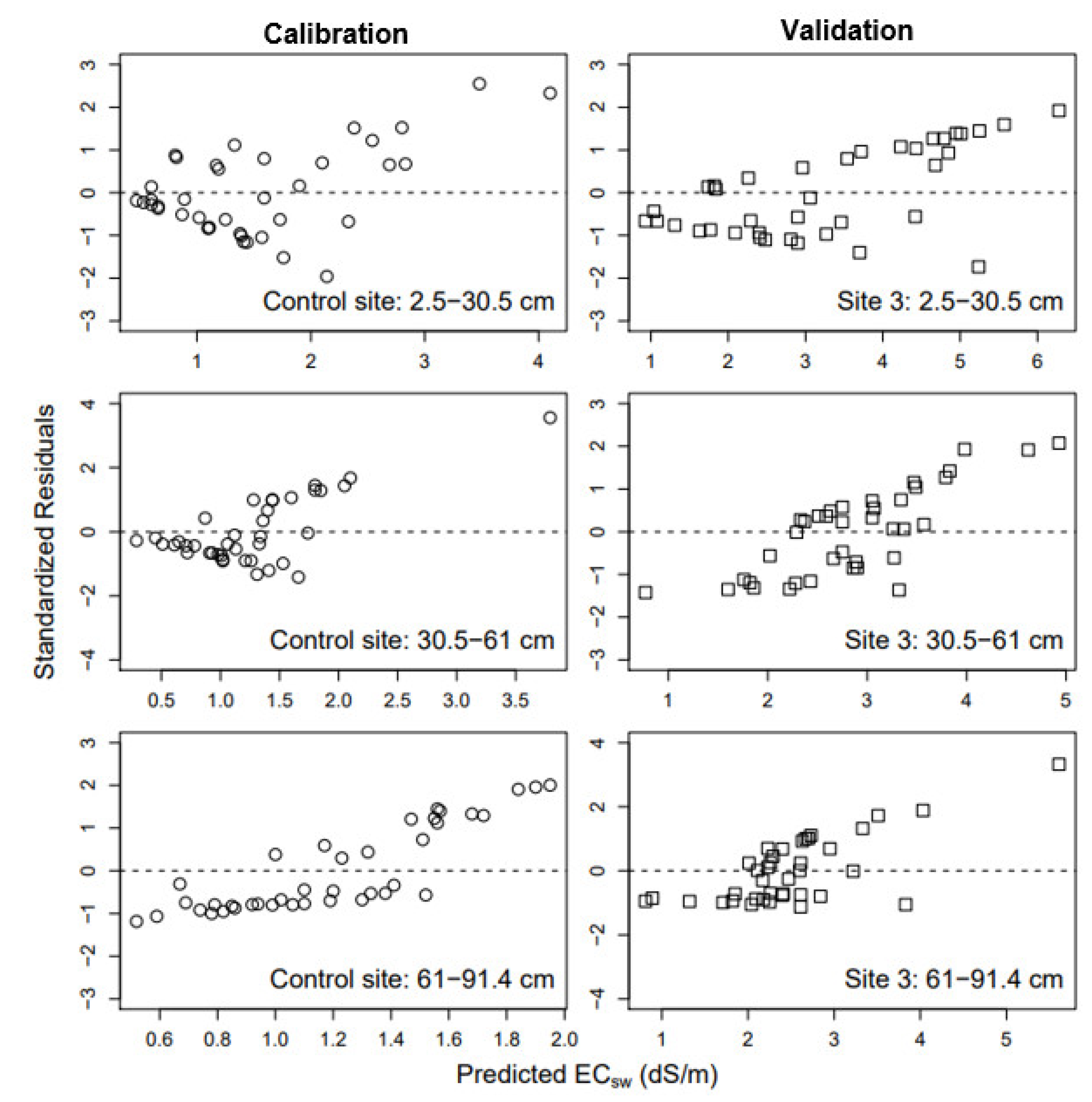
sw values greater than ~2 dS/m. Based on the relatively small MRE values that provide an indication of the magnitude of the error relative to observed values without considering the error direction, the model captures salinity dynamics for all layers in the root zone. However, the Figure 8 plot of residuals vs. predicted ECsw for the calibration and validation results exhibits heteroscedasticity, that is, residuals grow as the predicted ECsw values increase. Overall, this latter observation suggests that although the NSE, RMSE, and MRE statistics show that the model has some predictive capacity, it does not capture some processes apparently involved in the soil salinity dynamics.
The possible explanation for the differences in measured and predicted soil salinity is that the model does not account for fertilizer and soil amendment management, or plant root uptake of solutes and fertilizer. Generally, transformation (e.g., dissolution) in the soil of different chemicals added during fertigation will increase soil salinity. For example, urea is converted to ammonium that is adsorbed in the soil depending on sol temperature; ammonium is converted to nitrate by nitrification that depends on soil temperature, soil moisture, pH and oxygen content, and nitrate is highly mobile but ammonium, potassium, and phosphorus remain relatively immobile in the root zone. Although the salt index (SI) based on equivalent units of sodium nitrate (developed in 1943 to evaluate the salt hazard of fertilizers) alone cannot be used to evaluate the effect of increased soil salinity from fertilizer applications, it can be used as indicator for the long-term effects on soil salinity. The most commonly used fertilizers in the study region (from California Department of Food and Agriculture annual reports) were nitrogen fertilizers that included urea ammonium nitrate solution (SI = 95), ammonium nitrate (SI =102) and calcium nitrate (SI = 53); phosphorus fertilizer (SI = 7.8-29), potassium sulfate (SI = 46), gypsum, and lime. Sodium nitrate was arbitrarily set at 100, where EC of 0.5 to 40 mass percentage of sodium nitrate is 0.54 to 17.8 dS/m and for a mixture of materials it is reasonable to assume EC is additive for horticulture. As such, the lower the index value the smaller the contribution the fertilizer makes to the level of soluble salts. Thus, fertilizer applications likely add to soil salinities exacerbating the problem over time.
Although the model underestimates ECsw, it adequately captures salinity trends in the leaching of salt during winter months and an increase in salinity water applications and ET during the crop season. In an effort to evaluate performance of transient vs. steady state models, Reference [12] concluded that the transient models better predict the dynamics of the chemical–physical–biological interactions in an agricultural system. However, since we account for irrigation water salinity, rainfall salinity and dissolution of salts in the soil and exclude additions of fertilizer and soil amendment our simulated ECsw values can be viewed as a likely lower bound of soil salinity associated with the irrigation and farm management practices considered in the model description.
Another complexity possible affecting model prediction is the spatial distribution of salinity with drip irrigation as noted by Reference [59]. They used the transient Hydrus-2D model to compare results between field experiments having both drip and sprinkler irrigated processing tomatoes under shallow water table conditions for a wide range of irrigation water salinities. Both field and model results showed that soil-wetting patterns occurring under drip irrigation caused localized leaching which was concentrated near the drip line. In addition, a high-salinity soil volume was found near the soil surface that increased with increasing applied water EC. Overall, localized leaching occurred near the drip line while soil salinity increased with increasing distance from the emitter and with increasing soil depth. Such localized non-uniformities in leaching are not captured in the one-dimensional model but may have affected field soil sampling in the drip–irrigated fields of our study region. That is, soil samples collected some distance from where dripline emitters were previously operating would likely have greater salinities than would otherwise occur under the uniform leaching and dissolution conditions assumed in the model. Nonetheless, it is important to note that this model is user-friendly and less data intensive and it can be very useful for setting reference benchmarks of long-term salinity impacts of using saline water for irrigation.

3.3. Long-Term Salinity with Treated Wastewater Irrigation

We used the calibrated and validated model to simulate the long-term (50-year periods) soil salinity in the fields irrigated with varying fractions of treated wastewater, that is, we applied the model to control site and sites 2 to 7 (Table 2 and 
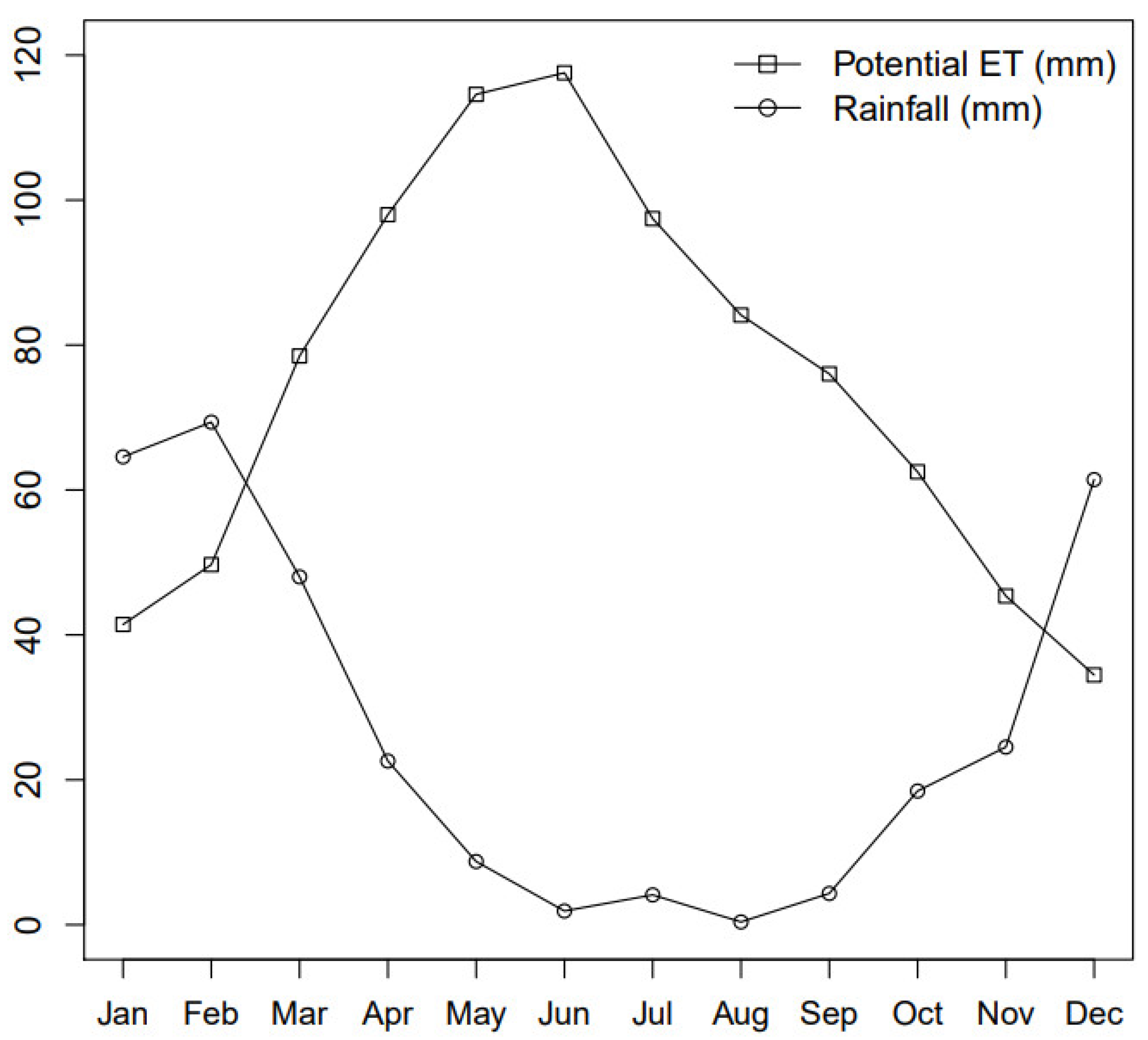
Table 3). Fifty-year simulations assumed randomly selected rainfall and ETo data from historical records (1983 to 2014) from 2013 to 2049 and the 13-year cropping patterns and irrigation management. In the model calibration, the groundwater table height (Hwt) and groundwater salinity (ECgw) were found to be non-influential parameters with respect to the measured soil water EC (ECsw). As such average values of measured Hwt and ECgw from the monitoring well located ~5 km west of the study site were used, that is, 0.95 m and 0.97 dS/m, respectively. For each simulated case, the three output variables of interest were averaged root zone salinity over the growing season expressed as ECeS (dS/m), annual drainage salt output load as Sd (kg/ha/year), and annual runoff salt output load Sr (kg/ha/year).
Values for the annual average water-balance terms over the 13-water year simulation at each site are summarized in Table 9a and for the 50-water year simulation in Table 9b. Somewhat greater actual crop water uptake (ET) is achieved under drip and sprinkler irrigated fields with similar crop rotations (sites 2 and 3 as compared to 6 and 7). Leaching fractions were generally very low for all sites at less than 2%. The greatest leaching occurred in the vegetable–strawberry rotation that was first sprinkler than drip irrigated, while the other irrigation and cropping practices yielded similar leaching volumes with the exception of no leaching from drip-irrigated artichokes. Similarly, surface runoff is smaller from drip or sprinkler irrigated fields as compared to sprinkler-furrow irrigated fields.
Simulated average (50-year) annual root zone soil water salinity for all sites is shown in Figure 9. Sites managed with sprinkler or drip irrigation and with higher salinity water (ECw) had higher estimated annual average ECsw, for example, at sites 3, 4, and 5, ECsw was 2.94 dS/m, 3.15 dS/m, and 3.44 dS/m, respectively. For sites 6 and 7 that used sprinklers for germination then furrow irrigation, the latter site received water with higher salinity than the former 1.37 dS/m compared to 1.1 dS/m on vegetable and strawberry rotation, but the resulting average annual soil water salinity differed little, that is, 2.05 versus 2.89 dS/m, respectively. The control site irrigated with well water had the least annual average rootzone soil–water salinity. Furthermore, soil–water salinity equilibrium ECsw ≤ 2.0 dS/m was reached throughout the 50-year horizon for the control site irrigated with well water and after 12 years of irrigated with blended wastewater for sites 2, 6, and 7, whereas for sites 3, 4, and 5 soil water EC increased above 2.0 dS/m in the simulation period. Using Mann–Kendall analysis we found that actual ET had a positive and significant association whereas irrigation amounts had a negative and significant association with ECsw ≤ 2.0 dS/m (Tau = 0.321, p-value = 0.016 and Tau = −0.268, p-value = 0.046 respectively). The Mann–Kendall Tau values indicate the strength and direction of monotonic trends, with −1 and 1 representing perfectly negative and positive monotonic trends, respectively, while the p-value indicates relative significance [60].
As Platts and Grismer [11] found that salt leaching to deeper soil layers occurred during the rainy season (October–March), while during the growing season soil–water EC increases in soil layers near the surface due to evapo-concentration, on the other hand, applied water salinity causes soil–water EC spikes during the growing season. Rainfall was important towards salt leaching from the root zone at all sites as evident during the wet years 2010, 2016, 2025, 2026, 2038, and 2046 when average annual soil water EC decreased. With the exception of sites 3, 4, and 5, there were no upward trends in soil water salinity over the 50-year period. Overall, relatively constant soil–water EC after 50 years simulation of ECsw < initial ECsw of 2.19 dS/m for all sites except site 5 suggest that there was adequate soil leaching in the region for sustained use of the treated wastewater for irrigation. However, the question remained as to what level of soil salinity would be acceptable especially for annual strawberry production.
Crops are generally assumed to respond to seasonal-averaged root zone salinity of the saturated paste (ECeS) and yield loss thresholds and rates of decline with increasing salinity have been determined based on salinity thresholds in [61]. We calculated EC
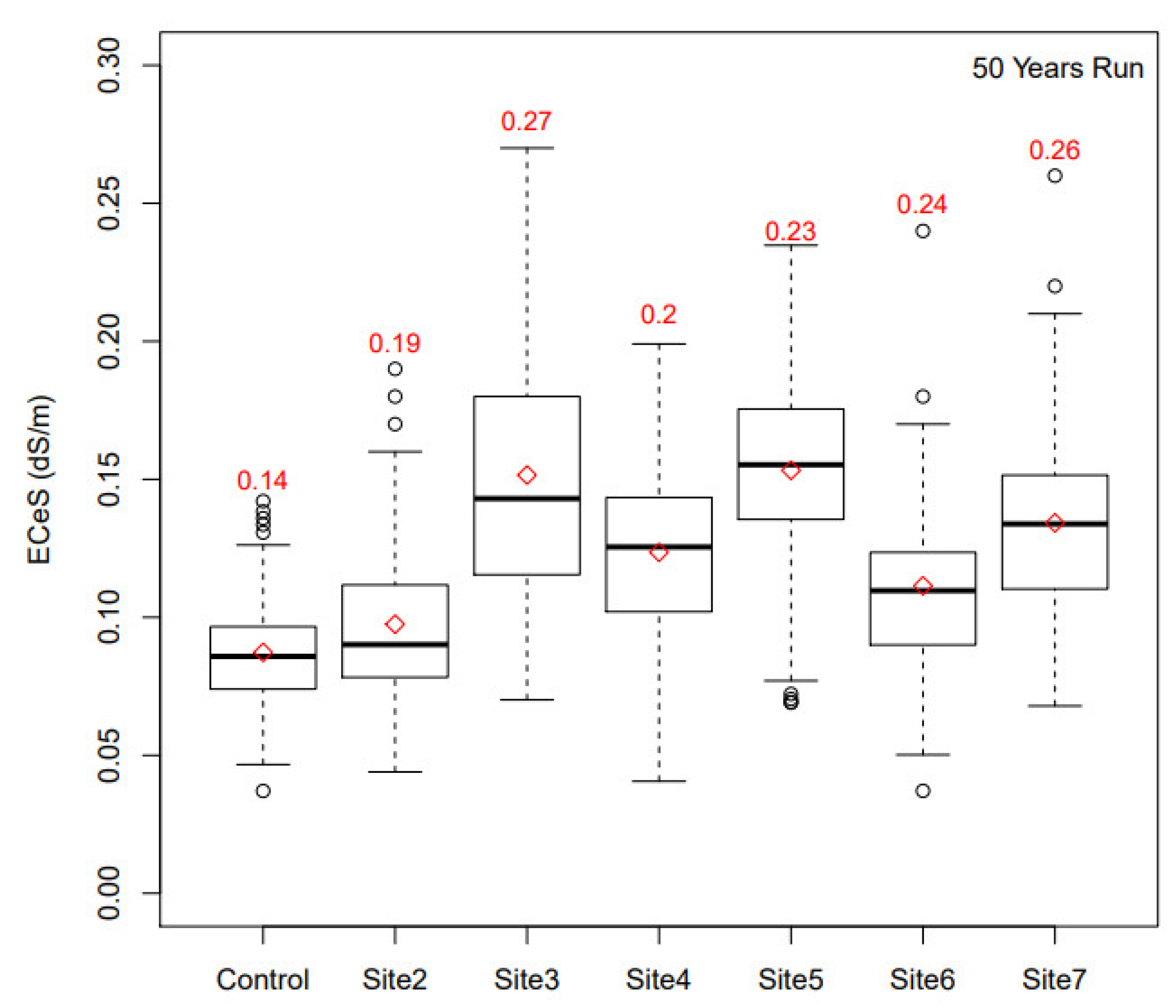
eS for all the sites and plot the range of ECeS in Figure 10. The maximum seasonal-averaged saturated paste EC for each site was 0.19, 0.27, 0.20, 0.23, 0.24, and 0.26 dS/m for sites 2, 3, 4, 5, 6, and 7, respectively. These values are less than half that of the lowest Mass–Hoffman threshold value of EC e = 1.0 dS/m associated the most sensitive crop (strawberry) in the rotations considered. As such, it is unlikely that long-term irrigation with treated wastewater in the region will adversely affect crop yields significantly.
In terms of possible adverse environmental effects associated with salinization of surface and ground waters in the region, we determined the cumulative salt output load with deep percolation (Sd) and salt output load with runoff (Sr) during the 50-water year simulation period for the different sites as shown in Figure 11. Salts accompanying surface runoff pose a larger threat in the watershed as these are an order-of-magnitude greater than the cumulative salt output loads to groundwater. Salt loading with deep percolation for the 50-year simulation range up to 3,377 kg/ha with the greatest loads from site 3 and minimal loading for sites 4 and 5 (40 kg/ha and 49 kg/ha respectively) on which annual artichoke crops were grown. Cumulative salt loads accompanying runoff ranged from 19,918 to 59,552 kg/ha, with the greatest loading emanating from site 3 and least from site 4. In comparison to the control site irrigated with well water cumulative salt output loading with deep percolation was 1325 kg/ha and salt output load with runoff 21,505 kg/ha.
To clarify what factors were key to affecting adverse environmental salinization within the region, we tested the effect of applied water EC (ECw) and depths, rainfall depths, actual crop ET and potential crop ET, and number of days fallow on soil water EC (ECsw) and salt output loads with runoff (Sr) or deep percolation (Sd) using the non-parametric Mann–Kendall trend analysis (the ‘Kendall’ test in the R package [60]. With respect to the Mann–Kendall Tau values (Table 10), the applied water EC (ECw) and rainfall depths had positive and significant effects on annual average soil water EC (ECsw) and annual salt output loads with runoff (Sr) and deep percolation (Sd). Calculated actual crop ET had a positive and significant effect on ECsw; this is expected as water uptake by the plant and evaporation leave salts behind. On the other hand, actual crop ET had a negative and significant effect on Sd, and had no significant effect on Sr. Applied water depths had positive and significant effect on Sd and Sr. The number of days fields were fallowed had a negative effect on ECsw and a positive effect on Sd and Sr. Overall, these observations were consistent with that expected from the field observations and described above.

4. Discussion

We calibrated and validated a modified root zone salinity model originally developed by Isidoro and Grattan [17], which was then applied to estimate long-term soil salinity in fields irrigated with treated wastewater. We conducted a global sensitivity analysis using the elementary effect/Morris and Sobol’s methods to first reduce the number of influential model parameters important to calibration and that need to be acquired from the field. Seven of the thirty-three model parameters were found to be critical to root zone soil salinity dynamics. These were parameters accounting for salt dissolution in the soil, root zone hydraulic parameters, and crop rooting depth. Model calibration resulted in a satisfactory fit to the observed field data; however, the model underestimated soil water salinity (ECsw), especially for large ECsw > 2 dS/m measured during the growing season. We attributed this error to the model’s failure to account for fertilizer and soil amendment applications and transformation thereof (e.g., gypsum dissolution) in the soil. In addition, drip irrigation leads to very localized variations in soil salinity that depend on the distance from the emitter that are not considered in the model and may have affected field soil sampling between plantings and harvests. Nonetheless, the model adequately captured soil–water EC trends that were congruent with observed data.
Sites irrigated with greater salinity water (ECw) combined with sprinkler or drip had greater estimated annual average soil–water salinity (ECsw). Sites that combined sprinkler irrigation for germination with furrow for the remaining development stages resulted in lower annual average ECsw in the root zone even when more saline irrigation water was applied. Rainfall played an important role in the leaching of salts from the root zone as during wet years average annual soil water EC decreased at all sites. Moreover, rainfall had a negative and significant effect on annual average root zone ECsw. We found that for all sites use of treated wastewater for irrigation over the 50-year period does not affect strawberry yields, the most salt sensitive of the crops in the rotations encountered. Overall irrigation water EC (ECw), rainfall amounts, actual calculated crop ET and the number of days fields were fallowed had significant effects on annual average soil water EC (ECsw). ECw, rainfall and actual crop ET effects were positive and fallowing decreased average root zone ECsw. On the other hand, irrigation amounts and number of days fallowed had positive and significant effects on salt output loads associated with runoff and deep percolation. Moreover, soil water salinity equilibrium ECsw ≤ 2.0 dS/m is reached throughout the 50-year horizon for the control site irrigated with well water and after 8, 9 and 14 years of irrigated with blended wastewater for sites 2, 6, and 7 respectively. For sites 3, 4, and 5 soil water EC increased above 2.0 dS/m in the simulation period. Actual ET had a positive and significant association whereas irrigation amounts had a negative and significant association with ECsw ≤ 2.0 dS/m.
While we believe that the modeling results can inform recommendations about irrigation management practices and for estimating salt output loading resulting from use of saline waters for irrigation, difficulties in linking field observations of soil salinity and model predictions remain troubling. However, since we account for irrigation water salinity, rainfall salinity, and dissolution of salts in the soil and exclude additions of fertilizer and soil amendment our simulated ECsw values are likely a lower bound of soil salinity associated with the irrigation and farm management practices considered in the modeling. Nonetheless, it is important to note that this model is user-friendly and less data intensive and it can be very useful for setting reference benchmarks of long-term salinity impacts of using saline water for irrigation.

Author Contributions

Conceptualization, P.Z. and M.G.; Data curation, P.Z. and M.G.; Formal analysis, P.Z.; Funding acquisition, M.G.; Investigation, M.G.; Methodology, P.Z., I.K. and M.G.; Project administration, M.G.; Resources, M.G.; Software, P.Z.; Supervision, I.K. and M.G.; Validation, P.Z. and M.G.; Visualization, P.Z.; Writing—Original draft, P.Z. and M.G.; Writing—Review & editing, I.K. and M.G.

Funding

The Monterey County Water Resources Agency funded the water and soil sampling monitoring program and collection of cropping data.

Acknowledgments

We thank Stephen Grattan and Daniel Isidoro for providing notes and equations for the root zone salinity model and Belinda Platts and the Monterey County Water Resources Agency for water and soil sampling and crop data.

Conflicts of Interest

The authors declare no conflict of interest.

Appendix A

Table A1. Cropping patterns for the control site and sites irrigated with treated wastewater.
Site #Cropping PatternCropPlanting MonthHarvest MonthAverage Growing Days
Control Lettuce, Broccoli, Cauliflower, CabbageLettuceMar–AugJun–Nov72
BroccoliJul–AugOct–Dec101
CauliflowerJul–NovApr–Oct118
CabbageAprJul98
2Lettuce, Broccoli, Cauliflower, Spinach, CeleryLettuceJan–SepApr–Nov74
BroccoliJan–JunMay–Oct104
CauliflowerMay–AugAug–Nov94
SpinachSepOct49
CeleryJulOct93
3Lettuce, Broccoli, Cauliflower, StrawberryLettuceMar–JulMay–Oct73
BroccoliFeb–JulJun–Oct104
CauliflowerFeb–AprMay–Jul94
StrawberryNovOct–Nov344
4 & 5Artichoke1st crop MayAnnual
2nd crop Oct–Nov
6Lettuce, Broccoli, Cauliflower, Strawberry, CeleryLettuceJan–JulApr– Sep74
BroccoliApr–JulJul–Oct92
CauliflowerJan–JulMay–Nov99
StrawberryNovNov344
CeleryMay–JulAug–Oct95
7Lettuce, Cauliflower, BroccoliLettuceMar–AugMay–Oct72
CauliflowerApr–AugJul–Aug92
BroccoliJulOct97
Table A2. Time-averaged crop coefficients and maximum rooting depth.
CropKc ValuesRooting Depth (cm)
InitialMidseasonLate
Artichoke0.510.9590
Broccoli0.71.050.9560
Cauliflower0.71.050.9570
Celery0.71.05150
Lettuce0.710.9550
Spinach0.70.90.9550
Strawberry0.40.90.8530
Figure A1. Crop rotation schedule for the control site and site 3.
Agriculture 09 00031 g0a1
Figure A2. Effect of salinity and sodium adsorption ratio of irrigation water on infiltration rate. (Modified from Reference [6] (p. 44)).
Agriculture 09 00031 g0a2

Appendix B

Unsaturated Soil Water Movement

The soil matric potential (ψ) was related to the volumetric water content (θ) by means of Equation (A1) [32]:
φ = φ s × ( θ θ s ) b
Where θs was the volumetric water content at saturation, ψs is the water entry potential or ‘‘saturation’’ water potential and b is the slope of the water retention curve on a logarithmic plot. For each soil type, b and ψs were calculated from the volumetric water content at field capacity and wilting point and their respective potentials in absolute value (ψFC = 316 cm and ψWP = 15,849 cm; so that pF (FC) = 2.5 and pF (WP) = 4.2). Taking logarithms, the expression of the potentials for FC and WP become linear equations:
log ( φ FC )   =   2.5   =   log φ s     b . log ( θ FC θ s ) log ( φ WP )   =   4.2   =   log φ s     b . log ( θ WP θ s )
from which, b and ψs are estimated. The unsaturated hydraulic conductivity for a given θ was given by:
K   =   K s × ( θ θ s ) 2 b + 3
where Ks is the saturated hydraulic conductivity. Thus, unsaturated flow between layers (U) can be calculated as:
U   =   K ( Δ φ Δ Z )
where ∆Z is the center to center simulation distance selected between layers and neglecting the gravitational gradient.

Crop Water Uptake

Non-stressed crop ET is calculated as:
ET c   =   K c × ET o
where Kc is the crop coefficient and varies with the crop development stages (Table A2) and ETo is the reference ET. Between cropping seasons, all ET or evaporation E was assumed to take place from the upper layer. For this period Kc was calculated from the mean interval between precipitation events of each month and the mean precipitation event in each month and ETo [38].
In each layer (k), the actual crop ET can be lower than ETc(k) due to water stress, which depends on the soil water content and the sensitivity of the crop to low water contents, accounted for through the crop-specific parameter p: the ratio of readily available soil water (RAW) to total available water (TAW) (p = RAW/TAW) [38]. When the soil water content (W(k)) in a layer fell below We(k) = WP + (1 − p) TAW, the ET from that layer actual crop ET(k) dropped below the ETc(k), and the actual ET of the layer was calculated as:
actual   crop   ET   =   K s × ET c
where Ks is a stress coefficient [38]:
K s   =   1 if   W ( k )   >   W e ( k ) W ( k )     W e ( k ) W e ( k )     WP ( k ) if   WP ( k )   <   W ( k )   <   W e ( k ) 0 , if   W ( k )   <   WP ( k )
when one layer was stressed during the growing season (W(k) < We(k)), the model allowed increase in the extraction coefficient of the lower layer to supply the ET demand of the day. The root zone water uptake pattern depends on irrigation frequency. Root uptake patterns were taken from [18,42,43].
Root length increase a function time is calculated as [45]:
L z   =   L o   +   ( L max     L 0 ) × ( t     t 0 2 ) ( t L max t 0   2 )
where L z is the rooting depth at time t, L o is the starting root depth, L max is the maximum root length, t L max time after planting when L max is reached and t o is time to reach 90% crop emergence. This is a linear root expansion; the method assumes that once half of the time required for crop emergence is passed by t o 2 , the rooting depth starts to increase from an initial depth L o till L max is reached.

Water Balance

Surface runoff for winter rainfall and a fraction of applied water is modelled using the SCS method. We define curve number (CN) associated with row crop cover for the growing season and bare soil for non-growing season from the SCS tables and calculate precipitation runoff as:
SR ( p )   =   0 if   P     0 . 2 S ( P     0 . 2 S ) 2 P   +   0 . 8 S if   P   >   0 . 2 S
where P is runoff producing precipitation and S is the potential maximum retention after runoff begins related to CN by:
S   =   254   × ( 100 CN     1 )
Daily water balance for the 4-layered root zone and 2-layered vadose zone is performed. To account for the slow water movement between layers for low water content below field capacity, a slow upward or downward flow U is calculated dependent upon the difference in matric potential between soil layers (Equations B4). In the first quarter of the root zone inflows and outflows include applied water (I) and rainfall (P), the drainage above field capacity (D (1)) to layer 2, actual crop ET and U. For the underlying root zone layers, inflows and outflows include drainage (D) from the overlying layer, U and actual crop ET and finally for the unsaturated layers below the root zone inflows and outflows include D and U.
When the soil water content in layer “k” is above field capacity, the excess water drains to the lower layer over a two-day period, the higher flow in the first day than the second. The fraction α of the excess water that drains the first day is calculated from the soil texture in the layer through an empirical relation obtained to match results presented by approximately 0.9 for sand, 0.85 for loam and 0.7 for clay [49]. Two arbitrary water contents were defined from field capacity to saturation for each layer Wa and Wb defined as:
W a   =   ( 1 α )   × ( W s     W FC )   +   W FC W b   =   ( 1 α )   × ( W S     W FC )   +   W FC
Drainage (D) is calculated as:
D   = α × ( W s     W FC ) if   W   >   W b   ( 1 α ) × ( W s W FC ) if   W a   <   W   <   W b W     W FC if   W   <   W a
where WFC and Ws define field capacity and saturation of a soil layer. After taking out actual crop ET and D outflows from the layer, we also need to account for upwards or downward movement of water (U) dependent upon the difference in matric potential between soil layers (Equation (A4)).

Salt Balance

Salt balance was performed in conjunction with the water balance assuming complete mixing of water entering each layer with that already stored in that layer. The electrical conductivity of water (EC) was used as an indicator of salinity, assuming implicitly that there was a unique relationship between EC and total dissolved solids (TDS) in these dilute solutions and that the EC behaves like a non-reactive solute. Salinity of the input waters (irrigation water (ECw) and precipitation (ECp)) must be known. The mass of salts in layer k (Z(k)) is estimated from the product ECsw(k) W(k), where ECsw is the electrical conductivity of the soil water in that layer. The mass of salts in layer k in day 1 (t + 1) results from the salinity in day 0 (or t) and the salt fluxes in day 1 that are added sequentially. Accounting for layer 1 for example is as follows: salts in I, P, and mineral dissolution (kd) are added to the salt mass in layer 1 to obtain Z a ( 1 ) 1 :
Z a ( 1 ) 1 =   Z ( 1 ) 0   +   EC w × I 1 + EC p × P 1 + k d
This results in a soil water concentration of:
EC sw a ( 1 ) 1 = Z a ( 1 ) 1 / ( W ( 1 ) 0   +   I 1   +   P 1 )
Drainage takes place with concentration EC sw a so that the new mass of salts is:
Z b ( 1 ) 1 =   Z a ( 1 ) 1   EC sw a ( 1 ) 1 × D ( 1 ) 1
and the new soil water concentration is:
EC sw b ( 1 ) 1 = Z b ( 1 ) 1 / ( W ( 1 ) t   +   I 1   +   P 1     D ( 1 ) 1 )
The soil at this state is evapo-concentrated by crop water uptake (actual crop ET):
EC sw c ( 1 ) 1 = Z b ( 1 ) 1 / ( W ( 1 ) t   +   I 1   +   P 1     D ( 1 ) 1     actual   crop   ET   ( 1 ) 1 )
The mass of salts in the slow flow U are then added or removed to obtain the final mass of salts in the layer:
Z ( 1 ) 1 = Z b ( 1 ) 1   U 1 2 ×   EC sw c ( 2 ) 1 if   U 1 2   <   0 Z b ( 1 ) 1 U 1 2 × EC sw c ( 1 ) 1 if   U 1 2   >   0
which allows for calculating the final soil water concentration:
EC sw ( 1 ) 1 = Z ( 1 ) 1 / W ( 1 ) 1

References

  1. Hillel, D. Salinity Managment for Sustainable Irrigation: Integrating Science, Environment, and Economics; The World Bank: Washington, DC, USA, 2000. [Google Scholar]
  2. USBR. Quality of Water—Colorado River Progress Report No. 24; U.S. Bureau of Reclamation: Salt Lake City, UT, USA, 2013.
  3. Rose, D.A.; Konukcu, F.; Gowing, J.W. Effect of water table depth on evaporation and salt accumulation from saline groundwater. Aust. J. Soil Res. 2005, 43, 565–573. [Google Scholar] [CrossRef]
  4. Grismer, M.E.; Gates, T.K. Estimating saline water table contributions to crop water use. Calif. Agric. 1988, 42, 23–24. [Google Scholar]
  5. Ragab, R.A.; Amer, F. Estimating water table contribution to the water supply of maize. Agric. Water Manag. 1986, 11, 221–230. [Google Scholar] [CrossRef]
  6. Hanson, B.R.; Grattan, R.R.; Fulton, A. Agricultural Salinity and Drainage; University of California, Davis: Davis, CA, USA, 2006. [Google Scholar]
  7. Konikow, L.F.; Rielly, T.E. Seawater intrusion in the United States. In Seawater Intrution in Coastal Aquifers; Bear, J., Cheng, A.H.D., Sorek, S., Ouazar, D., Herrera, I., Eds.; Springer: dordrecht, The Netherlands, 1999; pp. 463–506. [Google Scholar]
  8. Platts, B.E.; Grismer, M.E. Chloride levels increase after 13 years of recycled water use in the Salinas Valley. Calif. Agric. 2014, 68, 7. [Google Scholar] [CrossRef]
  9. MCWRA. State of the Salinas River Groundwater Basin; Monterey County Water Resources Agency: Salinas, CA, USA, 2015.
  10. Vengosh, A.; Gill, J.; Davisson, L.M.; Hudson, G.B. A multi-isotope (B, Sr, O, H, and C) and age dating (3H–3He and 14C) study of groundwater from Salinas Valley, California: Hydrochemistry, dynamics, and contamination processes. Water Resour. Res. 2002, 38, 9–1–9–17. [Google Scholar] [CrossRef]
  11. Platts, B.; Grismer, M.E. Rainfall leaching is critical for long-term use of recycled water in the Salinas Valley. Calif. Agric. 2014, 68, 75–78. [Google Scholar] [CrossRef]
  12. Letey, J.; Hoffman, G.J.; Hopmans, J.W.; Grattan, S.R.; Suarez, D.; Corwin, D.L.; Oster, J.D.; Wu, L.; Amrhein, C. Evaluation of soil salinity leaching requirement guidelines. Agric. Water Manag. 2011, 98, 502–506. [Google Scholar] [CrossRef]
  13. SHI National Soil Health Measurements to Accelerate Agricultural Transformation. Available online: http://soilhealthinstitute.org/national-soil-health-measurements-accelerate-agricultural-transformation/ (accessed on 23 August 2017).
  14. Maas, E.V.; Hoffman, G.J. Crop Salt Tolerance. J. Irrig. Drain. 1977, 103, 20. [Google Scholar]
  15. Rhoades, J.D.; Kandiah, A.; Mashali, A.M. The Use of Saline Waters for Crop Production; FAO: Rome, Italy, 1992; Volume FAO Irrigation & Drainage, p. 48. [Google Scholar]
  16. Shelia, V.; Simunek, J.; Boote, K.; Hoogenboom, G. Coupling DSSAT and HYDRUS-1D for simulations of soil water dynamics in the soil-plant-atmosphere system. J. Hydrol. Hydromech. 2018, 66, 232–245. [Google Scholar] [CrossRef]
  17. Isidoro, D.; Grattan, S.R. Predicting soil salinity in response to different irrigation practices, soil types and rainfall scenarios. Irrig. Sci. 2011, 29, 197–211. [Google Scholar] [CrossRef]
  18. Ayers, R.S.; Westcot, D.W. Water Quality for Agriculture; Food and Agriculture Organization of the United Nations: Rome, Italy, 1985. [Google Scholar]
  19. Gates, T.K.; Grismer, M.E. Stochastic approximation applied to optimal irrigation and drainage planning. J. Irrig. Drain. 1989, 115, 255–283. [Google Scholar] [CrossRef]
  20. Grismer, M.E. Pore-size distribution and infiltration. Soil Sci. 1986, 141, 249–260. [Google Scholar] [CrossRef]
  21. Ayars, J.; Christen, E.; Soppe, R.; Meyer, W. The resource potential of in-situ shallow groundwater use in irrigated agriculture. Irrig. Sci. 2006, 24, 147–160. [Google Scholar] [CrossRef]
  22. Grismer, M.E. Use of Shallow Groundater for Crop Production; UC Agriculture & Natural Resources: Davis, CA, USA, 2015; pp. 1–6. [Google Scholar]
  23. Grismer, M.E.; Bali, K.M. Subsurface drainage systems have little impact on water tables salinity of clay soils. Calif. Agric. 1998, 52, 18–22. [Google Scholar] [CrossRef]
  24. Grismer, M.E.; Gates, T.K.; Hanson, B.R. Irrigation and drainage strategies in saline problem areas. Calif. Agric. 1988, 42, 23–24. [Google Scholar]
  25. Talsma, T. The Control of Saline Groundwater; Meded, Landbouwhogeschool: Wageningen, The Netherlands, 1963; Volume 63, pp. 1–68. [Google Scholar]
  26. Durbin, T.J.; Kapple, G.W.; Freckleton, J.R. Two-Dimensional and Three-Dimensional Digital Flow Models of the Salinas Valley grouNd-Water Basin, California; Water Resources Division, US Geological Survey: Reston, VA, USA, 1978.
  27. Hall, P. Selected Geological Cross Sections in the Salinas Valley Using GeoBASE; Monterey County Water Resources Agency: Salinas, CA, USA, 1992.
  28. Fogg, G.E.; Labolle, E.M.; Weissmann, G.S. Groundwater Vulnerability Assessment: Hydrogeologic Perspective and Example from Salinas Valley, California. In Assessment of Non-Point Source Pollution in the Vadose Zone; American Geophysical Union: Washington, DC, USA, 2013; pp. 45–61. [Google Scholar]
  29. University of California, Division of Agriculture and Natural Resources. SoilWeb. Available online: https://casoilresource.lawr.ucdavis.edu/gmap/ (accessed on 7 October 2018).
  30. Šimůnek, J.; Šejna, M.; Saito, H.; Sakai, M.; van Genuchten, M.T. The Hydrus-1D Software Package for Simulating the Movement of Water, Heat, and Multiple Solutes in Variably Saturated Media; 4.14; Department of Environmental Sciences, University of California Riverside: Riverside, CA, USA, 2013. [Google Scholar]
  31. DWR CIMIS: California Irrigation Managemetn Information System. Available online: https://cimis.water.ca.gov/Resources.aspx (accessed on 6 April 2017).
  32. Clapp, R.B.; Hornberger, G.M. Empirical equations for some soil hydraulic properties. Water Resour. Res. 1978, 14, 601–604. [Google Scholar] [CrossRef]
  33. Brooks, R.H.; Corey, A.T. Hydraulic properties of porous media. In Hydrology Papers; Colorado State University: Fort Collins, CO, USA, 1964. [Google Scholar]
  34. Gardner, W.R. Some steady state solutions of unsaturated moisture flow equations with application to evaporation from a water table. Soil Sci. 1958, 84, 228–232. [Google Scholar] [CrossRef]
  35. Haverkamp, R.; Vaclin, M.; Touma, J.; Wierenga, P.J.; Vachaud, G. A comparison of numerical simulation models for one-dimensional infiltration. Soil Sci. Soc. Am. J. 1977, 41, 285–294. [Google Scholar] [CrossRef]
  36. Mualem, Y. A new model for predicting the hydraulic conductivity of unsaturated porous media. Water Resour. Res. 1976, 12, 513–522. [Google Scholar] [CrossRef]
  37. van Genuchten, M.T. A closed-form equation for predicting the hydraulic conductivity of unsaturated soils. Soil Sci. Soc. Am. J. 1980, 44, 892–898. [Google Scholar] [CrossRef]
  38. Allen, R.G.; Pereira, L.S.; Raes, D.; Smith, M. Crop evapotranspiration-Guidelines for computing crop water requirements-FAO Irrigation and drainage paper 56. FAO Rome 1998, 300, D05109. [Google Scholar]
  39. Hjelmfelt, A.T. Investigation of curve number procedure. J. Hydraul. Eng. 1991, 117, 725–737. [Google Scholar] [CrossRef]
  40. USDA. Natural Resources Conservation Service National Engineering Handbook; USDA: Washington, DC, USA, 2008; Volume Part 623 Section 15.
  41. Raats, P.A.C. Distribution of salts in the root zone. J. Hydrol. 1975, 27, 237–248. [Google Scholar] [CrossRef]
  42. Rhoades, J.D. Use of saline drainage water for irrigation. In Agricultural Drainage; Skaggs, R.W., van Schilfgaarde, J., Eds.; Agronomy Monograph, ASA-CSSA-SSSA: Madison, WI, USA, 1999; Volume 38, pp. 615–657. [Google Scholar]
  43. Skaggs, T.H.; Anderson, R.G.; Corwin, D.L.; Suarez, D.L. Analytical steady-state solutions for water-limited cropping systems using saline irrigation water. Water Resour. Res. 2014, 50, 9656–9674. [Google Scholar] [CrossRef]
  44. Grattan, S.R.; Grieve, C.M. Salinity–mineral nutrient relations in horticultural crops. Sci. Horticult. 1998, 78, 127–157. [Google Scholar] [CrossRef]
  45. Steduto, P.; Hsiao, T.C.; Raes, D.; Fereres, E. Crop yield Response to Water; Food and Agriculture Organization of the United Nations Rome: Rome, Italy, 2012. [Google Scholar]
  46. Orang, M.N.; Snyder, R. Consumptive Use Program-CUP+; California Department of Water Resources: Sacramento, CA, USA, 2013.
  47. Cahn, M. Estimated Crop Coefficients for Strawberry. In Salinas Valley Agriculture; UCANR: Salinas Valley, CA, USA, 2012; Volume 2017. [Google Scholar]
  48. Herman, J.; Usher, W. SALib: An open-source Python library for sensitivity analysis. J. Open Source Softw. 2017, 2, 97. [Google Scholar] [CrossRef]
  49. Hillel, D.; van Bavel, C.H.M. Simulation of Profile Water Storage as Related to Soil Hydraulic Properties. Soil Sci. Soc. Am. J. 1976, 40, 807–815. [Google Scholar] [CrossRef]
  50. DWR. California’s Groundwater Bulletin 118; California Department of Water Resources: Sacramento, CA, USA, 2004.
  51. Saltelli, A.; Ratto, M.; Andres, T.; Campolongo, F.; Cariboni, J.; Gatelli, D.; Saisana, M.; Tarantola, S. Global Sensitivity Analysis: The Primer; Wiley: Hoboken, NJ, USA, 2008. [Google Scholar]
  52. Morris, M.D. Factorial sampling plans for preliminary computational experiments. Technometrics 1991, 33, 161–174. [Google Scholar] [CrossRef]
  53. Campolongo, F.; Cariboni, J.; Saltelli, A. An effective screening design for sensitivity analysis of large models. Environ. Model. Softw. 2007, 22, 1509–1518. [Google Scholar] [CrossRef]
  54. Sobol′, I.M. Global sensitivity indices for nonlinear mathematical models and their Monte Carlo estimates. Math. Comput. Simul. 2001, 55, 271–280. [Google Scholar] [CrossRef]
  55. Saltelli, A. Making best use of model evaluations to compute sensitivity indices. Comput. Phys. Commun. 2002, 145, 280–297. [Google Scholar] [CrossRef]
  56. McKay, M.; Beckman, R.; Conover, W. A comparison of three methods for selecting values of input variables in the analyss of output from a computer code. Technometrics 1979, 21, 239–245. [Google Scholar]
  57. O’Geen, A. Reclaiming Saline, Sodic, and Saline-Sodic Soils. In Drought Tip; University of California, Agriculture and Natural Resources: Richmond, CA, USA, 2015. [Google Scholar]
  58. Mullen, K.; Ardia, D.; Gil, D.; Windover, D.; Cline, J. DEoptim: An R Package for Global Optimization by Differential Evolution. J. Stat. Softw. 2011, 40, 1–26. [Google Scholar] [CrossRef]
  59. Hanson, B.; Hopmans, J.W.; Simunek, J. Leaching with Subsurface Drip Irrigation under Saline, Shallow Groundwater Conditions. Vadose Zone J. 2008, 7, 810–818. [Google Scholar] [CrossRef]
  60. McLeod, A.I. Kendall, version 2.2; Univerity of Western Ontario: London, ON, Canada, 2015. [Google Scholar]
  61. Grieve, C.M.; Grattan, S.R.; Maas, E.V. Plant salt tolerence. In Angricultural Salinity Assessment and Management, 2nd ed.; Wallender, W.W., Tanji, K.K., Eds.; American Society of Civil Engineers: Reston, VA, USA, 2012; pp. 405–459. [Google Scholar]
Figure 1. Mean monthly rainfall (P) and reference ETo from the California Irrigation Management Information System (CIMIS) station 19 in Castroville, CA.
Agriculture 09 00031 g001
Figure 2. Annual rainfall and reference ETo from CIMIS station 19 in Castroville, CA.
Agriculture 09 00031 g002
Figure 3. Main components of the soil–water and salinity balance model across the soil–water–plant–atmosphere–aquifer continuum.
Agriculture 09 00031 g003
Figure 4. Workflow for calibration of the soil-water water and salt balance model.
Agriculture 09 00031 g004
Figure 5. Morris method µ* (the absolute of the mean elementary effect) values for soil depth layers. (a) 0.03–0.30 m; (b) 0.3–61 m; (c) 0.61–0.91 m depths.
Agriculture 09 00031 g005
Figure 6. Morris method µ* (the absolute of the mean elementary effect) vs. σ (the standard deviation of the elementary effect) for the different soil depths.
Agriculture 09 00031 g006
Figure 7. Predicted vs. measured ECsw at 2.5–30.5 cm, 30.5–61 cm and 61–91.4 cm soil depths for control site (calibration) and site 3 (validation).
Agriculture 09 00031 g007
Figure 8. Predicted ECsw vs. standardized residuals at 2.5–30.5 cm, 30.5–61 cm, and 61–91.4 cm soil depths for control site (calibration) and site 3 (validation).
Agriculture 09 00031 g008
Figure 9. Annual average soil–water salinity for sites irrigated with varying fractions of treated wastewater (2000 to 2049).
Agriculture 09 00031 g009
Figure 10. Range of estimated growing season saturated paste EC in the root zone for each site.
Agriculture 09 00031 g010
Figure 11. Cumulative salt output loads with runoff and deep percolation from each site.
Agriculture 09 00031 g011
Table 1. Average soil profile texture variations in the study region [29].
TextureDepth (m)Textural Fractions (%)Conductivity Ks (mm/d)Bulk Density (kg/m3)
SandClaySiltOM
Clay loam0–0.620–4527–3520–532121–3631660
Sandy loam0.6–0.935–7015–273–440.5363–12181640
Loam0.9–1.230–5020–2728–500.5363–12181640
Silty clay loam1.2–315–2027–3545–580.536–1211700
Table 2. Average electrical conductivity (EC) of applied water (ECw) at different sites from 2000–2012.
Site #2000–20092010–2012
% Recycled WaterECw (dS/m)% Recycled WaterECw (dS/m)
Control 00.6300.78
2460.75921.12
3941.52981.19
4580.94961.17
5931.511001.21
6701.14901.09
7961.56901.17
Table 3. Model parameters used in the sensitivity analysis. (Note: rz—root zone layers 1–4; 5—unsaturated zone layer 5; 6—unsaturated zone layer 6).
PropertyModel CodeModel UnitsRange
Min.Max.
Soil Hydraulic Parameters
Saturated water contentTsrzcm3/cm30.4390.486
Ts5cm3/cm30.3570.37
Ts6cm3/cm30.360.38
Water content at field capacityTfcrzcm3/cm30.3240.367
Tfc5cm3/cm40.2400.320
Tfc6cm3/cm50.2500.270
Water content at wilting pointTwprzcm3/cm30.1540.177
Residual water contentTr5cm3/cm50.110.14
Tr6cm3/cm50.0660.08
Saturated hydraulic conductivityKsrzcm/day12.136.3
Ks5cm/day36.3121.8
Ks6cm/day3.612.1
Fraction of excess water drained the first dayArz%0.810.83
A5%0.850.87
A6%0.80.82
Runoff Curve Number for fallow periodsCNf-9194
Growing season Curve Number CNc-8891
Capillary fridge height above the water tableHdcm83183
Depth to groundwater tableHwtM7.4511.57
Depth of surface soil layer subjected to drying by evaporation Zemm100150
Plant Parameters
Root water uptake for layers 1–3RWU1%6071
RWU2%2030
RWU3%67
Rooting depth of lettuce, broccoli, cabbage and cauliflowerZrLcm3050
ZrBrccm4060
ZrCabbcm5080
ZrCaucm4070
Fraction of total available water that can be depleted from the root zone before moisture stress for lettucepL-0.30.7
Fraction of total available water that can be depleted from the root zone before moisture stress for broccoli, cabbage, and cauliflowerpBCC-0.450.7
Soil Chemical Parameter
Rate of dissolution at 2.5–30.5 cm depthk1dSm−1/day00.014
Rate of dissolution at 30.5–61 cm depthk2dSm−1/day00.022
Salinity at shallow water tableECgwdSm−10.351.58
Initial ECswECswdSm−10.294.1
Table 4. Sampling sizes and number of model runs performed for each sensitivity analysis method.
MethodSample SizeModel Evaluations
Elementary Effect (EE) w/10 trajectories1000340
Sobol’s10200
11220
12240
Table 5. Parameter sensitivity based on Morris indices.
CodeParameterµ*µµ*_ConfΣ/EE
Root zone Sampling Depth of 0.03–0.3 m
k1Rate of dissolution at 0.03–0.30 m depth 0.16−0.140.070.15
ZrLRooting depth of lettuce0.1−0.100.060.1
TsrzRoot zone saturated water content0.09−0.070.080.14
KsrzRoot zone saturated hydraulic conductivity0.080.030.060.12
TwprzRoot zone water content at wilting point0.05−0.050.030.05
HdCapillary fringe height 0.040.040.080.12
pLFraction of depletable moisture for lettuce0.040.030.020.04
Root zone Sampling Depth of 0.30–0.61 m
k1Rate of dissolution at 0.03–0.30 m depth0.12−0.10.070.13
KsrzRoot zone saturated hydraulic conductivity0.07−0.030.040.11
TsrzRoot zone saturated water content0.07−0.050.060.12
Tfc5Unsaturated zone saturated water content0.05−0.020.040.08
k2Rate of dissolution at 0.3–0.61 m depth0.05−0.050.020.04
ZrLRooting depth of lettuce0.05−0.040.030.06
TwprzRoot zone water content at wilting point0.04−0.020.020.05
HdCapillary fringe height 0.040.030.060.1
Tr5Unsaturated zone residual water content0.03−0.030.020.04
Root zone Sampling Depth of 0.61–0.91 m
k1Rate of dissolution at 0.03–0.30 m depth0.13−0.080.060.16
TsrzRoot zone saturated water content0.09−0.050.060.14
KsrzRoot zone saturated hydraulic conductivity0.08−0.010.060.13
Tfc5Unsaturated zone saturated water content0.06−0.030.060.11
TwprzRoot zone water content at wilting point0.05−0.030.030.07
HwtDepth to groundwater table0.050.050.060.1
ZrLRooting depth of lettuce0.05−0.040.040.07
k2Rate of dissolution at 0.3–0.61 m depth0.05−0.040.030.04
HdCapillary fringe height 0.040.040.070.13
Tr5Unsaturated zone residual water content0.03−0.030.020.04
µ* is a good proxy of the total sensitivity index [53].
Table 6. Sobol’s sensitivity indices.
CodeParameterSTST_confSiSi_conf
Root zone Sampling Depth of 0.03–0.3 m
k1Rate of dissolution at 0.03–0.30 m depth0.650.420.420.33
ZrLRooting depth of lettuce0.430.47−0.100.29
TfcrzUnsaturated zone saturated water content0.070.06−0.040.13
KsrzRoot zone saturated hydraulic conductivity0.050.08−0.010.06
TsrzRoot zone saturated water content0.040.05−0.070.11
TwprzRoot zone water content at wilting point0.020.02−0.080.07
k2Rate of dissolution at 0.3–0.61 m depth0.010.010.030.05
HwtDepth to groundwater table0000.02
HdCapillary fringe height 0000.02
Root zone Sampling Depth of 0.30–0.61 m
TsrzRoot zone saturated water content3.389.10.010.11
k1Rate of dissolution at 0.03–0.30 m depth0.860.530.310.5
k2Rate of dissolution at 0.3–0.61 m depth0.270.190.280.28
ZrLRooting depth of lettuce0.240.490.030.24
TfcrzUnsaturated zone saturated water content0.050.0600.14
KsrzRoot zone saturated hydraulic conductivity0.040.070.010.13
TwprzRoot zone water content at wilting point0.020.02−0.030.07
HwtDepth to groundwater table00.01−0.020.05
HdCapillary fringe height 00.01−0.020.05
Root zone Sampling Depth of 0.61–0.91 m
k1Rate of dissolution at 0.03–0.30 m depth0.890.680.050.44
ZrLRooting depth of lettuce0.360.480.050.21
k2Rate of dissolution at 0.3–0.61 m depth0.290.170.090.24
TsrzRoot zone saturated water content0.120.220.020.08
KsrzRoot zone saturated hydraulic conductivity0.070.1−0.030.08
TfcrzUnsaturated zone saturated water content0.060.070.030.1
TwprzRoot zone water content at wilting point0.030.03−0.010.04
HdCapillary fringe height 00.0100.01
HwtDepth to groundwater table00.0100.01
Table 7. Best-fit parameter values estimated with calibration for ECsw.
PropertyCodeUnitsValue
Soil Hydraulic Parameters
Root zone saturated water content Tsrzm3/m30.467
Root zone water content at field capacityTfcrzm3/m30.361
Root zone water content at wilting pointTwprzm3/m30.172
Root zone saturated hydraulic conductivityKsrzmm/day347
Plant Parameters
Rooting depth of lettuceZrLm0.5
Soil–Water Chemistry Parameters
Rate of dissolution at 0.03–0.30 m k1dSm−1/day0.014
Rate of dissolution at 0.30–0.61 m k2dSm−1/day0.022
Table 8. Statistical indices for simulated vs. observed soil water EC (ECsw).
IndexRMSEMRENSER2b
Optimal value00111
Control Site (Calibration)
0.03–0.30 m0.450.230.720.730.89
0.30–0.61 m0.410.250.520.520.89
0.61 – 0.91 m0.340.260.160.270.95
Site 3 (Validation)
0.03–0.30 m0.950.240.560.600.87
0.30–0.61 m0.700.210.240.390.88
0.61–0.91 m0.600.200.480.510.94
Table 9. Summary of annual average water balance and salinity variables for the different field management scenarios.
a. 13 Years Simulations
Site No.Control Site234567
Crop managementVegetablesVegetablesVegetables and strawberryPerennial artichokeVegetables and strawberryVegetables
Irrigation managementSprinkler then dripSprinkler or dripSprinkler then dripSprinkler or dripSprinkler then furrowSprinkler then furrow
Irrigation (mm/yr)652597682648694656
Seasonal Evapotranspiration ET (mm/year)254200252392204177
Surface runoff (mm/year)299232236158315265
Leaching (mm/yr)7.14.416.3023.712.7
Irrigation water electrical conductivity ECW (dS/m)0.710.941.361.061.361.11.37
Root zone ECSW (dS/m)1.481.742.452.42.891.761.95
Root zone seasonal-averaged electrical conductivity of the saturated extract ECeS (dS/m)0.090.130.190.150.180.150.17
Salt output load with deep percolation Sd (kg/ha/year)614220700153104
Salt output load with runoff Sr (kg/ha/year)3048511860648101210731465
b. 50 Years Simulations
Site No.Control Site234567
Seasonal ET (mm/year)187128188395141131
Surface runoff (mm/year)323295236163275250
Leaching (mm/year)8.07.29.41.013.08.8
ECW (dS/m)0.710.941.361.061.361.11.37
Root zone ECSW (dS/m)1.121.201.862.052.521.341.50
Root zone ECeS (dS/m)0.140.190.270.200.230.240.26
Sd (kg/ha/year)2720640.81.05638
Sr (kg/ha/year)3054911028339518598764
Table 10. Mann–Kendall trend analysis for average annual soil water EC (ECsw), annual salt output load with runoff (Sr), and with deep percolation (Sd).
ParameterECsw (dS/m)Sr (kg/ha/year)Sd (kg/ha/year)
Taup-Value aTaup-Value aTaup-Value a
ECw (dS/m)0.33***0.49***0.04ns
Rainfall (mm/year)−0.18*0.03ns0.06ns
Potential crop ET (mm/year)0.03ns0.24**0.17*
Actual crop ET (mm/year)0.44***−0.11ns−0.33***
Irrigation (mm/yr)0ns0.41***0.24**
Days fallow (days)−0.44***0.26**0.39***
a Two-sided p-value ranges: 0 ≤ *** ≤ 0.001; 0.001 < ** ≤ 0.01; 0.01 < * ≤ 0.05; ns > 0.05.

