
Risk Coupling Assessment of Vehicle Scheduling for Shipyard in a Complicated Road Environment

School of Ocean and Civil Engineering, Shanghai Jiao Tong University, Shanghai 200240, China
*
Author to whom correspondence should be addressed.
J. Mar. Sci. Eng. 2024, 12(4), 685; https://doi.org/10.3390/jmse12040685
Submission received: 24 March 2024
/
Revised: 15 April 2024
/
Accepted: 17 April 2024
/
Published: 22 April 2024
(This article belongs to the Special Issue Risk Assessment in Maritime Transportation)
Abstract
:Vehicle scheduling at shipyards can involve delays due to numerous risk factors encountered in the complicated shipyard road environment. This paper studies the problems of risk coupling in shipyard vehicle scheduling based on the risk matrix approach, considering the complicated road environment, assessing the degrees of coupling and disorder. Based on safety-engineering theory and comprehensive analysis of the road environment, four key criteria are identified, vehicles, the road environment, the working environment, and humans, including 12 factors and their specific contents. The degree of coupling between various combinations of risk criteria is quantitatively determined utilizing the N-K model. Additionally, the degree of disorder in the risk criteria is assessed based on information entropy theory. The model’s correction coefficients are determined through comparative analysis of experimental data. By integrating the degree of coupling and disorder, delays caused by different combinations of risk criteria in scheduling tasks are computed. The quantitative evaluation model enables accurate appraisal of risk events during shipyard vehicle scheduling. The model provides a valuable managerial tool to analyze delays caused when specific risk criteria are met and to compare these delays to the potential impact on time resulting from adjusting vehicle scheduling plans. This research has significant implications for enhancing vehicle distribution efficiency in shipyards.
1. Introduction
Large cruisers manufactured in shipyards are custom-designed and constructed, and their reliance on standardized components is significantly lower than that of automobiles built in factories. Furthermore, a substantial proportion of the hull components used in shipbuilding requires individualized processing within shipyards. Additionally, owing to the generally non-mechanical nature of ship construction, extensive labor is required, which poses significant challenges in terms of material management. The construction of large cruise ships entails a vast number of components, estimated at tens of millions [1,2]. For example, Adora Magic City, currently under construction in China, comprises 503 thin-plate structural segments and requires the assembly of approximately 25 million individual parts. Given the number and magnitude of these components, efficient and precise vehicle scheduling for shipyards (VSS) is crucial. The coordination and management of VSS, which encompasses various stages, are typically undertaken by the companies themselves. This involves the organization of fleets and establishment of distribution routes [3]. Although this approach to distribution offers benefits in terms of centralized management and increased operational efficiency, it also features drawbacks such as substantial investment requirements, diminished flexibility, and elevated risk levels.
Typically, for materials of great significance, a reliable logistics distribution service is essential. It is crucial that such goods are transported without any damage or deterioration, because such occurrences could result in the loss of the goods’ original properties, leading to the failure in meeting production-plan requirements [4]. Furthermore, timely delivery in accordance with production schedules is paramount to ensure that materials are not delivered prematurely or delayed [5,6]. When considering various logistics and distribution modes, it is important to note that the higher the number of handling, loading, and unloading processes during transit, the greater the likelihood of cargo damage. Similarly, a large number of intermediate links within the logistics mode introduces greater uncertainty regarding the timing of deliveries [7]. This uncertainty encompasses various risk events, including those related to vehicles, road conditions, working environments, and human factors, which can have a detrimental impact on vehicle scheduling [8]. Furthermore, these effects are often inadequately assessed, leading to a lack of effective managerial responses to these risk factors. To effectively assess the impact of these risk factors on vehicle scheduling, in the context of the complicated shipyard road environment, this paper studies the problems of risk coupling in the context of VSS.
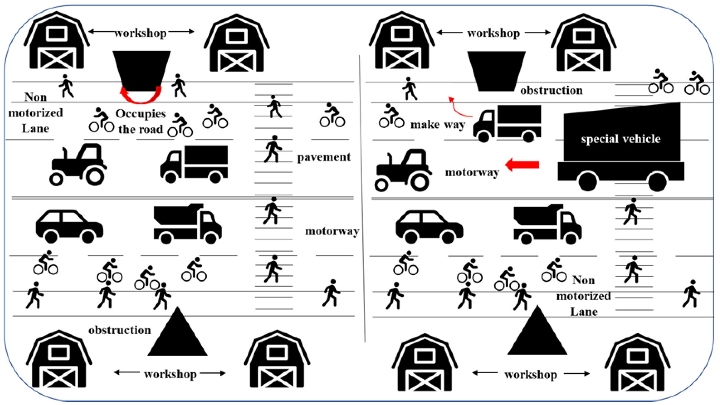
Vehicles within shipyards comprise both motorized and non-motorized vehicles. Furthermore, it is important to note the presence of pedestrians on roadways. Motorized vehicles are categorized into production vehicles and non-production vehicles. There are seven types of production vehicle, including flatbed trucks, aerial trucks, forklifts, tractor trucks, car cranes, trucks, and battery forklifts [9]. Non-production vehicles are divided into commuter cars, private cars, and commercial vehicles. Owing to the substantial and intensive nature of production tasks within shipyards, both motorized vehicles and non-motorized vehicles are frequently used on shipyard roads during working days. The intersection of various vehicles on shipyards is characterized by a high level of complexity, which distinguishes such roads from environments in public areas. Moreover, shipyard roads are assigned managers who are responsible for their supervision and management. The specific nature of vehicular movement within shipyards involves a higher frequency of overtaking maneuvers, placing a greater emphasis on drivers’ situational awareness compared with that in public areas despite the fact that, overall, the speeds at which vehicles travel in these areas is lower than on regular roads. This latter factor also contributes to vehicular congestion within shipyard environments. In the shipyard, the bicycle is the predominant non-motorized vehicle and provides a high level of convenience. However, conflicts frequently occur between non-motorized and motorized vehicles, particularly in areas where roads are narrow. The large volume of bicycles occupying non-motorized vehicle lanes frequently results in traffic congestion and encroachment into motorized-vehicle lanes. This leads to lane-changing and overtaking maneuvers between bicycles and motorized vehicles that ultimately reduce the capacity of motorized-vehicle lanes. Shipyard roads also include pedestrian pathways and sidewalks, which pedestrians navigate in a random manner, often moving in multiple directions. In the presence of pedestrians on sidewalks, motorized vehicles are often required to take evasive measures to ensure a safe driving environment. However, these circumstances require adaptations in the distribution efficiency. Additionally, the distinctions between shipyard vehicles and typical road vehicles extend to specialized flatbed trucks used for transporting medium-sized ship products (Figure 1). Given the considerable dimensions of these products, flatbed trucks occupy multiple lanes during their operation. As a result, other vehicles are required to yield way, often leading to notable scheduling delays. Consequently, the shipyard road environment is often chaotic owing to the diverse array of vehicle types, compounded by the presence of pedestrians.
Another contributing factor in the complexity and disorderliness of shipyard roads is the existence of workshops. These workshops, each with specific functionalities, are located on both sides of shipyard roads [10]. During their operational phases, the workshops produce various levels of noise, which has a significant impact on drivers’ and marshals’ attentiveness [11]. Furthermore, ship segments are occasionally temporarily placed on the roads, which reduces the available driving space and exacerbates disorderly road environments, with pedestrians and bicycles further restricting the flow of motorized traffic (Figure 1).
In this study, the N-K model is utilized to quantify the degree of coupling among risk factors, while information entropy theory is applied to assess the level of road congestion during scheduling. Subsequently, the two models are integrated to establish a quantitative model that calculates the degree of impact of risk factors. The contributions of this study are threefold: (1) the formation mechanism of vehicle distribution risk for shipyards is formulated based on the characteristics of shipyard roadways; (2) an innovative risk assessment model combining the N-K model and information entropy theory is developed to quantitatively evaluate the duration of delays of vehicle delivery caused by risk factors; and (3) the duration of delays is added, which is the sum of the degree of coupling and the degree of disorder.
Literature Review
Researchers investigating transportation risk predominantly utilize mathematical models and methodologies to quantitatively determine the probability and magnitude of the impact of risks. These models are applied to provide guidance to decision makers or managers regarding the implementation of necessary safety measures [12]. Since it was first proposed in 1970, the quantitative risk assessment method has been extended to the transportation industry [13,14]. However, given transportation studies in shipyards are uncommon, the research reviewed in this paper includes transportation studies in other industries. In general, quantitative risk studies focus on the following: (a) calculation of the probability of risk (CPR) [15,16,17]; (b) calculation of the risk-impact level (CRIL) [18,19]; (c) the combined model of risk probability and impact level (CMRPIL) [20,21,22]; and (d) the improvement in risk models (IRM) [23,24]. This section of this paper is devoted to a review of the literature on CMRPIL and IRM.
CMRPIL and IRM have been widely used in many areas, such as sustainable integrated logistics and the transportation industry. Yang et al. [25] propose a risk diffusion model integrating a motion mechanism to implement multiple-granularity traffic risk evaluation. Shankar et al. [26] proposed an integrated risk-assessment model based on intuitionistic fuzzy set theory and D-number theory to assess risk in freight-transportation systems. Karatzetzou et al. [27] used the multi-hazard risk-assessment model to analyze probabilities in transportation networks, while Chakrabarti and Parikh [28] evaluated risk in hazmat transportation using the HAZAN methodology. Additionally, Yang et al. [29] innovatively develop Non-Negative Matrix Factorization (NMF) to explore the quantitative risk under the coupling of multiple risk factors for traffic safety evaluation. Finally, Ambituuni et al. [30] developed a framework for regulatory improvement to assess risk in the context of transportation by road. These risk studies are based on the definition of risk as a combination of the probability of the risk factors being encountered and the consequences thereof. The process of the calculation of risk can be defined as the quantification of risk index in the arithmetic pattern other than logic implication as follows [31]: Risk = Severity × Probability. Probability and severity have different definitions depending on the object of study. The calculation of risk probabilities and severity in many studies is based on expert knowledge, leading to subjective results. Extant studies have focused more on the influence of risk in distribution processes and rarely examine the influence of the impact on tasks; furthermore, they rarely analyze risk factors based on the road environment. In the actual road environment, not all risk factors are encountered throughout; therefore, the impact of different combinations of risk factors on the distribution tasks needs to be considered.
2. Materials and Methods
The proposed integrated assessment model is implemented to quantitatively assess the risk in VSS. A flowchart of the risk coupling analysis of VSS is shown in Figure 2. Once the assessment criteria and factors are identified, the number of risk factors resulting from each criterion over a period of time can be counted. Using these data, we calculate the degree of coupling of risk criteria based on the N-K model. Based on the combination probability calculated in the N-K model, the confusability of the combined risk factors can be calculated based on information entropy theory. Next, the correction coefficient is calculated to obtain the final quantitative evaluation model. Finally, the model is used to evaluate delays in VSS.
2.1. Hybrid Risk Coupling Model Based on Risk Matrix Approach
The formula for the combined risk coupling model proposed is based on the risk matrix approach [31], which is considered a combination of the severity of the consequences S and their probability P [32]. In this article, vehicle scheduling risk for shipyards is defined based on the combination of risk criteria that cause delays in scheduling tasks.
Through comprehensive analysis of shipyard road environments, distinct characteristics of VSS can be identified, leading to the formulation of the following definitions:
Definition 1.
Complexity represents the extent of the intricate interrelationships or associations observed between diverse types of criteria, denoted as the degree of coupling, C(x).
Definition 2.
Disorderliness encompasses the intricacy or complexity inherent in the operational environment of a vehicle, notably including the road and work surroundings. Disorderliness is designated as the degree of disorder, H(x).
The risk of delays arising from vehicle scheduling tasks cannot be solely attributed to the cumulative delays resulting from various risk criteria. Rather, the risk is intricately linked to the interplay between various risk criteria and road characteristics. In this paper, we add the result of risk, H, which is the sum of the degree of coupling and the degree of disorder.
Hence, we propose Equation (1) as a means of assessing the delays associated with diverse combinations of risk criteria. Equation (1) contains the form of the combination of different risk criteria and the quantitative characteristics of shipyard roads. In Equation (1), S is the total delay of the risk criteria; Tcar represents the average delays resulting from inherent risk conditions specific to the vehicle; Troad denotes the average delays caused by risk conditions pertaining to the road; Twork signifies the mean delays attributed to environmental influencing vehicles; Tother represents the temporal influence exerted by additional risk criteria, including pedestrian-related criteria; Ts denotes the long-term repercussions, such as noise-related effects, of work activities that generate noise; and represents the correction coefficient.
This paper increases the weight of the degree of coupling and the degree of disorder. The formula is not only a simple summation of the degree of coupling and disorder, because the calculation of the degree of disorder utilizes the probability of the degree of coupling. Finally, we modify the model as follows:
where , representing the average delay caused by the combination of risk factors. , , and , indicating the characteristics of the transportation environment that influence vehicle distribution.
This is subject to
Equations (2) and (3) represent combinations of criteria, with a maximum of three and a minimum of no combinations of the various criteria occurring.
The relationship between the models is illustrated in Figure 3. The N-K model calculates the probability values of risk factors for different combinations, which can be applied to the calculation of the coupling values and to information entropy theory. Information entropy theory can be used to calculate the confusion value of the portfolio risk factors, which should be applied to the probability values. Section 2.2 and Section 2.3 introduce the N-K model and information entropy theory, respectively.
2.2. Calculating the Degree of Coupling of Risk Criteria Based on the N-K Model
The N-K model, which was originally proposed based on fitness-landscape theory to study the evolution of organisms, has good generalizability in solving complex problems [33]. Many studies quantify risk-causing coupling based on objective accident data [34]. The N-K model contains two important parameters, where N represents the number of subsystems that make up the system, such that when there are n kinds of states in the subsystem, the number of states in the system is nN, while K represents the number of interdependencies in each subsystem in the system’s relationship network and determines the magnitude of the system’s adaptation. In this study, N is the number of risk criteria, and K represents the number of interacting risk criteria. n has two states, where “0” indicates the non-occurrence of a risk factor, “1” represents the occurrence of a risk factor, and “.” designates that the state is not constrained, “0” or “1”. The N-K model is calculated as follows:
where x1 = (1, 2, …, H1); x2 = (1, 2, …, H2); xn = (1, 2, …, Hn); Px1x2…xn represents the probability of the coupling of different criteria occurring in state xi; (x1, x2, …, xn) x, Px1, P•x2, …, P•••xn indicates the sum of the probability of the occurrence of n standard couplings when the standard is in the state xi; and C(Xn) denotes the degree of coupling under criteria n.
2.3. Calculating the Degree of Disorder of Risk Criteria Based on Information Entropy Theory
The information measure is the information created by a specific event that has occurred, while the entropy measure refers to the amount of information that can be expected to be generated before the result is known [35]. Entropy considers all possible values of the random variable and is the amount of information that can be expected to result from all possible events. Information can be understood as the probability of occurrence of a particular kind of information (i.e., the probability of the occurrence of discrete random events). In systems with high levels of order, the information entropy tends to be lower, whereas in systems characterized by increased chaos, information entropy tends to be higher [13]. Information entropy can be considered a quantitative measure of the level of organization, or order, within a system. In this paper, information entropy is used to determine the degree of disorder in various combinations of risk criteria.
where p(xi) denotes the probability of occurrence of event xi, and H(x) is the degree of confusion in event xi. In this paper, because p(xi) represents the probability of the combined events, we calculate it as follows:
where p(x1x2…xn) is the probability of the combined event (x1x2…xn) and is the probability of the occurrence of all events. Then, H(x) is calculated as follows:
3. Analysis of the Criteria and Factors for Risk Events in VSS
In safety engineering theory, risks can be classified into the following criteria: human, machine, materials, environment, and management [36]. Since shipyard vehicle transportation processes do not involve dangerous materials or management failures, we have limited our assessment to the following criteria: machine, environment, and human. In this paper, the term “machine” pertains to the failure of a vehicle. Huang et al. [36] define environment as bad weather and the condition of the roads. However, as evidenced by the comprehensive analysis presented in Section 1, the shipyard environment exhibits a profound level of complexity. Therefore, this paper meticulously divides the environment into distinct categories, encompassing both the road environment and the working environment. The road environment is defined as the presence of risk factors on the road, including other vehicles, pedestrians [37], and obstacles. The working environment is defined as encompassing bad weather conditions [38] and risk factors emanating from other work activities, particularly noise in this paper. Drivers who perform frequent high-risk events (e.g., hard braking maneuvers) pose a significant threat to traffic [39]. The present study classifies these high-risk event attributes as human.
To investigate the factors that contribute to delays, we also conducted a survey of workstations and engaged in consultations with twelve workers, five of whom possessed a decade of experience and seven who had accrued no more than five years of expertise. Eventually, we summarize the information pertaining to these criteria as follows.
Vehicle: Vehicles play a considerable role in scheduling tasks. Because shipyard materials vary significantly in type and volume, it is difficult to transport them using manpower alone. Therefore, vehicles are the main carriers in shipyard material distribution. Table 1 shows the details of some risk events encountered during the distribution of vehicles. The Internet of Vehicles (IOV) is a system used by the shipyard to track and record incidents involving vehicles. Column 4 shows the shipyard’s documentation of factors that pose a risk to vehicle operations in the IOV. Based on the IOV, we identified six types of vehicle-related risks that cause delays in scheduling tasks: maintenance, oil leakage, tank, steering arm, tire, and network. We counted the number of vehicle-related risk events resulting from each factor and from multiple factors. According to our investigation, these factors resulted in an average delay of 30 min for scheduling tasks.
Road Environment: Shipyard roads carry vehicles and therefore feature different kinds of vehicles and obstacles to public roads. In shipyard roads, target vehicles are significantly influenced by the other vehicles present on the road during scheduling tasks. Obstacles and pedestrians can further narrow the road, which can lead to additional task delays, as shown in Table 2. Therefore, we identify other vehicles and obstacles as the factors of road environment. These two factors exert a significant influence on the extension of the duration of a task, resulting in delays of approximately 15 min.
Working Environment: The factors of the working environment include noise and unfavorable weather. In Equation (1), Ts is defined as a long impact time, with a duration of persistence as long as the working day. Noise, serving as a significant risk factor, has a persistent presence throughout the working environment, encompassing sounds emanating from vehicles, workers, and other sources. This noise can potentially impact workers’ concentration levels and the dissemination of critical information. Noise is therefore classified as Ts, which affects the delay tasks by 5 min. Changes in climate can also affect transportation systems. Because shipyards are built beside the sea, unfavorable weather can occur, mainly in the form of wind or rain, which increases delays in the completion of tasks by 15 min, as shown in Table 3.
Human: In a shipyard road, many uncertainties in human behavior can affect driving. Human behavior is complex and variable, and therefore we do not attempt to categorize it here. Human does not belong to Ts, and this delays tasks by 15 min.
By analyzing the four types of risk factors, this paper determines the inputs and outputs of information and the average delay time of each criterion in a risk event, as shown in Table 4.
4. Analysis of Coupling of Risk Criteria in VSS
4.1. Definition of Risk Criteria Coupling in VSS
In physics, the interaction of two or more individuals or forms of motion is called “coupling”. Risk coupling is the phenomenon whereby interactions between factors within a system produce changes in the stability and risk level of the system. In a system, risk coupling is the result of nonlinear interactions between factors and can be viewed as a part of the system. Therefore, the interaction of vehicles, the road environment, the working environment, and humans in the vehicle distribution process is analyzed qualitatively from the perspective of risk criteria coupling in VSS.
We identify the historical frequency of occurrence of vehicles (C), the road environment (R), bad weather (W), and human errors (H), as well as the coupling between these risk criteria, in the quantitative assessment model mentioned above. Thereafter, we calculate the coupling probability. We use Nc, r, w, h, c {0, 1}, r {0, 1}, w {0, 1}, and h {0, 1} to represent the historical occurrence frequency and Pc, r, w, h, Nc, r, w, h, c {0, 1}, r {0, 1}, w {0, 1}, and h {0, 1} to denote the probability of coupling of each criterion, where C is in state c, R is in state r, W is in state w, and H is in state h.
4.2. Definition of Risk Criteria Coupling in VSS
Figure 4 illustrates the coupling mechanism of the VSS system. Based on the number of different categories of risk criteria involved in the coupling, the risk coupling of the VSS system can be divided into four categories, including single-criteria risk coupling, pairwise-interacting risk criteria, three-interacting risk criteria, and four-interacting risk criteria. The coupling values can change as the number of criteria in the combination increases.
(1) Single-criteria risk coupling
Single-criteria risk coupling refers to the risk arising from the interaction between risk criteria within a certain category of criteria, whose coupled action risk causes an increase in the level of systemic risk. The total coupling value is expressed by Pc (Vehicle), Pr (Road Environment), Pw (Working Environment), and Ph (Human).
(2) Pairwise-interacting risk criteria
Pairwise-interacting risk criteria refer to the interaction of two categories of risk criteria that affect the safety of VSS. Pc, r, Pc, w, Pc, h, Pr, h, Pr, w, and Pw, h show the risk change value of double-criteria risk coupling in each state. For example, Pc, r denotes the combination of Vehicle and Road Environment.
(3) Three-interacting risk criteria
Three-interacting risk criteria refer to the interaction of three categories of risk criteria that affect the safety of VSS. The total coupling value is expressed by Pc, r, h, Pc, r, w, Pc, w, h, and Pr, w, h. For example, Pc, r, h denotes the combination of Vehicle, Road Environment, and Human.
(4) Four-interacting risk criteria
Four-interacting risk criteria refer to the interaction of four categories of risk criteria that affect the safety of VSS. The total coupling value is expressed by Pc, r, w, h, which denotes the combination of all criteria.
5. Case Application and Results
5.1. Risk Database
In this study, the selected target vehicle for the shipyard is the flatbed truck. Using this type of vehicle, we investigate 288 delays caused by risk factors of a shipyard in Shanghai in 2022, as shown in Table 5. We divide the criteria of Vehicle and Road Environment into different categories and conduct a statistical analysis of the frequency of occurrence of delay risk for each factor. Owing to the extensive diversity and complexity of the categorization of the working environment and human, we conduct a macroscopic enumeration of the incidence of delayed risks. The frequency levels of the four risk criteria are denoted as 24.66%, 24.20%, 25.11%, and 26.03%, and they exhibit a minimal degree of variance. Within the domain of vehicular criteria, maintenance and steering arm represent a significantly larger proportion of the total. Within the road environment, other vehicles and pedestrians constitute a substantial proportion of the overall total. Noise accounts for a relatively large proportion of the total because of the potential for noise generation from workshops.
5.2. Analysis of Coupling Value and Disorder Value
The number and frequency of the different criteria are shown in Table 6. For example, Nc=1,r=0,w=0,h=0 is expressed as the frequency of occurrence of Vehicle only, and = .
Using the data in Table 6, we calculate the probability of a change in risk for the different interaction-risk criteria, as shown in Table 7, Table 8, Table 9 and Table 10. For example, Pc=0 = Pc=0,r=0,w=0,h=0 + Pc=0,r=1,w=0,h=0 + Pc=0,r=0,w=1,h=0 + Pc=0,r=0,w=0,h=1 + Pc=0,r=1,w=1,h=0 + Pc=0,r=1,w=0,h=1 + Pc=0,r=0,w=1,h=1 + Pc=0,r=1,w=1,h=1 = 0 + 0.0521 + 0.0625 + 0.0417 + 0.0313 + 0.0521 + 0.0833 + 0.1042 = 0.4272. These results are applied to calculate the degree of coupling C(x) and degree of disorder H(x).
Applying Equations (1) and (7), we calculate the degree of coupling and the degree of disorder for each combination, respectively, as shown in Table 11. In this paper, based on expert recommendations that both A and B hold equal significance, their respective weights are assigned as 0.5 each. We take the calculated coupling value as the degree of coupling of vehicle distribution. Using Equation (7) and taking the combination of A and B as an example, DC can be calculated by
H(C, R) = −Pc=1log (Pc=1) + (−Pr=1log (Pc=1)) + (−Pc=1, r=1log (Pc=1, r=1)) = 0.1386 + 0.1424 + 0.1579 = 0.4389
Figure 5 shows the variation in values for different combinations. Figure 6 shows the summation of DD and DC for different interaction risk criteria. The probabilities of the combined risk criteria are displayed in Figure 7. The results in Figure 5, Figure 6 and Figure 7 indicate the following: (a) The risk level of the system increases as the number of risk criteria increases. FIRC causes the greatest risk, followed by TIRC; furthermore, the higher the number of risk criteria involved in coupling, the greater the severity of a vehicle-operation-risk event. (b) As the number of combination criteria increases, the values of DC and DD increase, indicating that the environment in which the vehicle is transported is becoming more complex and chaotic. (c) The value of DD is greater than that of DC, indicating that the vehicle is operating in a more chaotic environment. (d) In the pairwise-interacting risk criteria, C (R, W) > C (W, H) > C (C, R) > C (C, H) > C (R, H) > C (C, W); accordingly, the road environment and the working environment affect the vehicle scheduling task to an increased extent because the road environment and the working environment in both combinations reach their maximal values. (e) C(R, W, H) > C(C, R, W), indicating that the combination of road environment, working environment, and human causes a higher risk of delays. (f) C(C, R, W) > C(C, W, H) > C(C, R, H), denoting that the working environment and the road environment can contribute to a higher risk of delays in combination with vehicles. (g) The probability of a vehicle operational risk event decreases as more risk criteria are involved in coupling.
5.3. Calculation of Coefficient
Based on the current operational conditions, the risk-event delay times for various combinations were recorded for the period from July 2022 to October 2022, as shown in Table 12. In Equation (1), the acquisition of the optimal adjustment coefficient is essential to determine the cumulative delay time. The aim of the optimization objective function in this study is to minimize the error between the actual measured time Ta and the theoretically calculated time Tr, from which the optimal value is identified. The formula for is as follows:
In this study, 12 groups of data are selected, with Group Delay_Time_1 to Group Delay_Time_10 treated as the experimental groups, while Group Delay_Time_11 and Group Delay_Time_12 serve as the control group. Based on the equation and the statistical data, the specific optimization equation can be derived as follows:
Proposition 1.
When takes values between 0 and 1, can be used to obtain the minimum value.
Proof.
Consider any , where Ta, (Ti, car•a + Ti, road•b + Ti, work•c + Ti, s), and (0.5•C(x)i + 0.5•H(x)i) are constants. Therefore, we assume that Ta, (Ti, car•a + Ti, road•b + Ti, work•c + Ti, s), and (0.5•C(x)i + 0.5•H(x)i) are A, B, and E respectively. Then, = . When , obtains the minimum value. We calculate the values of for groups 1 through 10, as shown in Table 13. □
In this paper, we take the average of as the value of , i.e., = (0.7404 + 0.7657 + 0.7185 + 0.7576 + 0.7912 + 0.7489 + 0.7325 + 0.7324 + 0.8089 + 0.7156)/10 = 0.7511.
Finally, the optimal value of is 0.7511, which is substituted into Equation (1) to derive the equation expressing the total impact on time due to each criterion being met:
5.4. Consequence Analysis of Risk Criteria
The theoretical delays for each combination of events are calculated using Equation (9), as shown in Table 14. In this study, we use the Group Delay_Time_11 and Group_Delay_Time_12 of the data as the control group to verify the reliability of the theoretical data obtained by using R2. R2 is a measure of the goodness of fit of the regression model, R2(0, 1). As the value approaches 1, the model’s reliability increases correspondingly. The values of R2 for Delay_Time_11, Delay_Time_12, and theoretical delay time were 0.8886 and 0.8519, which proves that the results are reliable. Figure 8 depicts a comparative analysis of the data from delays, Delay_Time_11, Delay_Time_12, and average delay time, indicating minimal discrepancy between the three outcomes. This can be attributed to the ability of the quantitative evaluation model to handle risk criteria efficiently.
6. Conclusions and Future Research Directions
In this research, we present a novel quantitative framework for the assessment of risk criteria occurring in shipyard vehicle scheduling. The proposed model offers a comprehensive means of evaluating the impact of such risk events on scheduling tasks by quantifying the associated delay time. The proposed model is superior to other methods in that it incorporates more criteria and registers the real-time delays triggered by risk criteria. The availability of such information can enable managers to devise a wider range of strategies to cope with potential risks.
Based on safety engineering theory and the shipyard environment, four criteria that affect scheduling tasks are identified: vehicles, the road environment, the working environment, and human factors. These criteria, including 12 factors and their specific content, are described in detail. Furthermore, we conduct an in-depth exploration of the average duration of the delays attributed to these criteria in scheduling tasks. Based on historical occurrences of the risk events, we count the number of occurrences of each criterion, and calculate the DC of different risk-combination times using the N-K model. In addition, based on information entropy theory, we calculated the DD in the risk criteria. Our analyses reveal the following:
- (1)
- The risk level of the system increases as the number of risk criteria increases. Therefore, managers should avoid developing vehicle scheduling plans during times when multiple risk criteria occur.
- (2)
- Roadway environments and working environments have a significant and substantial impact on the execution of vehicle scheduling tasks. When developing vehicle scheduling plans, it is imperative to take into account the conditions of the roadway environment. Given the ongoing nature of vehicle scheduling, it is advisable to reconsider and potentially modify the vehicle distribution plan when risk criteria manifest in real-time.
By comparing the experimental results, we calculated the correction coefficients in the quantitative model. The R2 values for the control groups and theoretical delay time are 0.8886 and 0.8519, respectively, which proves that the results are reliable. This finding has practical implications for the real-time scheduling of vehicles. Specifically, it suggests that if a risk criterion is met, the manager should analyze the delay caused by the risk and compare it to the potential delay resulting from adjusting the scheduling plan. For instance, if the delay caused by the risk exceeds the impact on timeliness resulting from changing the scheduling plan, a revised scheduling plan should be adopted. This approach can minimize the potential consequences of the risk. Overall, this quantitative model provides a reasonable and efficient approach to analyzing the delays in scheduling tasks due to risk criteria, making it an effective tool for analysis of these risk criteria.
Although this study makes several useful contributions, a limitation is that the present model is designed for shipyard scheduling; therefore, its suitability for analyzing risk in other industries requires verification. Nevertheless, the research framework established in this study can be used as a reference for other studies, which is a valuable contribution of our research. Furthermore, the findings of this study can be employed to enhance the scheduling of vehicles in shipyards. This involves developing more efficient strategies and algorithms to systematically formulate rational plans for real-time vehicle scheduling in response to fulfillment of risk criteria.
Author Contributions
J.Y.: Methodology, Investigation, Funding Acquisition, Formal Analysis, Conceptualization. N.W.: Writing—Original Draft Preparation, Methodology, Formal Analysis, Data Curation. J.Y., R.U.K. and N.W.: Writing—Review and Editing, Resources, Investigation. All authors have read and agreed to the published version of the manuscript.
Funding
This research was supported by the Ministry of Industry and Information Technology (China) for research on the key technology of the high-tech ocean passenger ship construction logistics collection system [MC-202009-Z03].
Institutional Review Board Statement
Not applicable.
Informed Consent Statement
Not applicable.
Data Availability Statement
The data presented in this study are available on request from the corresponding author.
Acknowledgments
The authors are thankful to all experts for providing their opinions and useful discussions. In addition, the authors are also thankful to Shanghai Waigaoqiao Shipbuilding Co. Ltd., China.
Conflicts of Interest
The authors declare no conflicts of interest.
References
- Dixit, V.; Verma, P.; Raj, P.; Sharma, M. Resource and time criticality based block spatial scheduling in a shipyard under uncertainty. Int. J. Prod. Res. 2018, 56, 6993–7007. [Google Scholar] [CrossRef]
- Ge, Y.; Wang, A.M. Spatial scheduling for irregularly shaped blocks in shipbuilding. Comput. Ind. Eng. 2021, 152, 106985. [Google Scholar] [CrossRef]
- Tao, N.R.; Jiang, Z.H.; Qu, S.P. Assembly block location and sequencing for flat transporters in a planar storage yard of shipyards. Int. J. Prod. Res. 2013, 51, 4289–4301. [Google Scholar] [CrossRef]
- Zheng, Y.H.; Ke, J.C.; Wang, H.Y. Risk Propagation of Concentralized Distribution Logistics Plan Change in Cruise Construction. Processes 2021, 9, 1398. [Google Scholar] [CrossRef]
- Sahin, B.; Yazir, D.; Soylu, A.; Yip, T.L. Improved fuzzy AHP based game-theoretic model for shipyard selection. Ocean Eng. 2021, 233, 109060. [Google Scholar] [CrossRef]
- Khalilzadeh, M.; Banihashemi, S.A.; Bozanic, D. A Step-By-Step Hybrid Approach Based on Multi-Criteria Decision-Making Methods And A Bi-Objective Optimization Model To Project Risk Management. Decis. Mak. Appl. Manag. Eng. 2024, 7, 442–472. [Google Scholar] [CrossRef]
- Kwon, B.; Lee, G.M. Spatial scheduling for large assembly blocks in shipbuilding. Comput. Ind. Eng. 2015, 89, 203–212. [Google Scholar] [CrossRef]
- Cui, Z.M.; Wang, H.Y.; Xu, J. Risk Assessment of Concentralized Distribution Logistics in Cruise-Building Imported Materials. Processes 2023, 11, 859. [Google Scholar] [CrossRef]
- Alfnes, E.; Gosling, J.; Naim, M.; Dreyer, H.C. Exploring systemic factors creating uncertainty in complex engineer-to-order supply chains: Case studies from Norwegian shipbuilding first tier suppliers. Int. J. Prod. Econ. 2021, 240, 108211. [Google Scholar] [CrossRef]
- Crispim, J.; Fernandes, J.; Rego, N. Customized risk assessment in military shipbuilding. Reliab. Eng. Syst. Saf. 2020, 197, 106809. [Google Scholar] [CrossRef]
- Adams, N.; Chisnall, R.; Pickering, C.; Schauer, S.; Peris, R.C.; Papagiannopoulos, I. Guidance for ports: Security and safety against physical, cyber and hybrid threats. J. Transp. Secur. 2021, 14, 197–225. [Google Scholar] [CrossRef]
- Brown, D.F.; Dunn, W.E. Application of a quantitative risk assessment method to emergency response planning. Comput. Oper. Res. 2007, 34, 1243–1265. [Google Scholar] [CrossRef]
- Koçar, O.; Dizdar, E. A risk assessment model for traffic crashes problem using fuzzy logic: A case study of Zonguldak, Turkey. Transp. Lett. Int. J. Transp. Res. 2022, 14, 492–502. [Google Scholar] [CrossRef]
- Li, Y.T.; Xu, D.D.; Shuai, J. Real-time risk analysis of road tanker containing flammable liquid based on fuzzy Bayesian network. Process Saf. Environ. Prot. 2020, 134, 36–46. [Google Scholar] [CrossRef]
- Bianco, L.; Caramia, M.; Giordani, S. A bilevel flow model for hazmat transportation network design. Transp. Res. Part C-Emerg. Technol. 2009, 17, 175–196. [Google Scholar] [CrossRef]
- Goksu, S.; Arslan, O. A quantitative dynamic risk assessment for ship operation using the fuzzy FMEA: The case of ship berthing/unberthing operation. Ocean Eng. 2023, 287, 115548. [Google Scholar] [CrossRef]
- Qiu, S.Q.; Sacile, R.; Sallak, M.; Schoen, W. On the application of Valuation-Based Systems in the assessment of the probability bounds of Hazardous Material transportation accidents occurrence. Saf. Sci. 2015, 72, 83–96. [Google Scholar] [CrossRef]
- Ahmadi, O.; Mortazavi, S.B.; Pasdarshahri, H.; Mohabadi, H.A. Consequence analysis of large-scale pool fire in oil storage terminal based on computational fluid dynamic (CFD). Process Saf. Environ. Prot. 2019, 123, 379–389. [Google Scholar] [CrossRef]
- Noguchi, H.; Hienuki, S.; Fuse, M. Network theory-based accident scenario analysis for hazardous material transport: A case study of liquefied petroleum gas transport in japan. Reliab. Eng. Syst. Saf. 2020, 203, 107107. [Google Scholar] [CrossRef]
- Khanmohamadi, M.; Bagheri, M.; Khademi, N.; Ghannadpour, S.F. A security vulnerability analysis model for dangerous goods transportation by rail—Case study: Chlorine transportation in Texas-Illinois. Saf. Sci. 2018, 110, 230–241. [Google Scholar] [CrossRef]
- Li, Y.L.; Yang, Q.; Chin, K.S. A decision support model for risk management of hazardous materials road transportation based on quality function deployment. Transp. Res. Part D-Transp. Environ. 2019, 74, 154–173. [Google Scholar] [CrossRef]
- Tao, L.L.; Chen, L.W.; Ge, D.C.; Yao, Y.T.; Ruan, F.; Wu, J.; Yu, J. An integrated probabilistic risk assessment methodology for maritime transportation of spent nuclear fuel based on event tree and hydrodynamic model. Reliab. Eng. Syst. Saf. 2022, 227, 108726. [Google Scholar] [CrossRef]
- Oturakci, M.; Dagsuyu, C. Integrated environmental risk assessment approach for transportation modes. Hum. Ecol. Risk Assess. 2020, 26, 384–393. [Google Scholar] [CrossRef]
- Satish, A.S.; Mangal, A.; Churi, P. A systematic review of passenger profiling in airport security system: Taking a potential case study of CAPPS II. J. Transp. Secur. 2023, 16, 8. [Google Scholar] [CrossRef]
- Yang, L.; Luo, X.K.; Zuo, Z.J.; Zhou, S.P.; Huang, T.Y.; Luo, S. A novel approach for fine-grained traffic risk characterization and evaluation of urban road intersections. Accid. Anal. Prev. 2023, 181, 106934. [Google Scholar] [CrossRef] [PubMed]
- Shankar, R.; Choudhary, D.; Jharkharia, S. An integrated risk assessment model: A case of sustainable freight transportation systems. Transp. Res. Part D-Transp. Environ. 2018, 63, 662–676. [Google Scholar] [CrossRef]
- Karatzetzou, A.; Stefanidis, S.; Stefanidou, S.; Tsinidis, G.; Pitilakis, D. Unified hazard models for risk assessment of transportation networks in a multi-hazard environment. Int. J. Disaster Risk Reduct. 2022, 75, 102960. [Google Scholar] [CrossRef]
- Chakrabarti, U.K.; Parikh, J.K. Applying HAZAN methodology to hazmat transportation risk assessment. Process Saf. Environ. Prot. 2012, 90, 368–375. [Google Scholar] [CrossRef]
- Yang, H.Y.; Zhao, X.H.; Luan, S.; Chai, S.S. A traffic dynamic operation risk assessment method using driving behaviors and traffic flow Data: An empirical analysis. Expert Syst. Appl. 2024, 249, 123619. [Google Scholar] [CrossRef]
- Ambituuni, A.; Amezaga, J.M.; Werner, D. Risk assessment of petroleum product transportation by road: A framework for regulatory improvement. Saf. Sci. 2015, 79, 324–335. [Google Scholar] [CrossRef]
- Ni, H.H.; Chen, A.; Chen, N. Some extensions on risk matrix approach. Saf. Sci. 2010, 48, 1269–1278. [Google Scholar] [CrossRef]
- Božanić, D.; Pamučar, D.; Komazec, N. Applying D numbers in risk assessment process: General approach. J. Decis. Anal. Intell. Comput. 2023, 3, 286–295. [Google Scholar] [CrossRef]
- Huang, W.C.; Yin, D.Z.; Xu, Y.F.; Zhang, R.; Xu, M.H. Using N-K Model to quantitatively calculate the variability in Functional Resonance Analysis Method. Reliab. Eng. Syst. Saf. 2021, 217, 108058. [Google Scholar] [CrossRef]
- Zhang, W.J.; Zhang, Y.J. Research on coupling mechanism of intelligent ship navigation risk factors based on N-K model. J. Mar. Sci. Technol. 2023, 28, 195–207. [Google Scholar] [CrossRef]
- Pele, D.T.; Lazar, E.; Dufour, A. Information Entropy and Measures of Market Risk. Entropy 2017, 19, 226. [Google Scholar] [CrossRef]
- Huang, W.C.; Zhang, Y.; Yu, Y.C.; Xu, Y.F.; Xu, M.H.; Zhang, R.; De Dieu, G.J.; Yin, D.Z.; Liu, Z.R. Historical data-driven risk assessment of railway dangerous goods transportation system: Comparisons between Entropy Weight Method and Scatter Degree Method. Reliab. Eng. Syst. Saf. 2021, 205, 107236. [Google Scholar] [CrossRef]
- Shaaban, K.; Muley, D.; Mohammed, A. Analysis of illegal pedestrian crossing behavior on a major divided arterial road. Transp. Res. Part F Traffic Psychol. Behav. 2018, 54, 124–137. [Google Scholar] [CrossRef]
- Zainuddin, N.I.; Arshad, A.K.; Hamidun, R.; Haron, S.; Hashim, W. Influence of road and environmental factors towards heavy-goods vehicle fatal crashes. Phys. Chem. Earth Parts A/B/C 2022, 129, 103342. [Google Scholar] [CrossRef]
- Zhang, R.C.; Wen, X.; Cao, H.Q.; Cui, P.F.; Chai, H.; Hu, R.B.; Yu, R.Y. High-risk event prone driver identification considering driving behavior temporal covariate shift. Accid. Anal. Prev. 2024, 199, 107526. [Google Scholar] [CrossRef]
Figure 1.
Road environment of shipyard.

Figure 2.
Flowchart of assessment of risk coupling in shipyard vehicle scheduling.
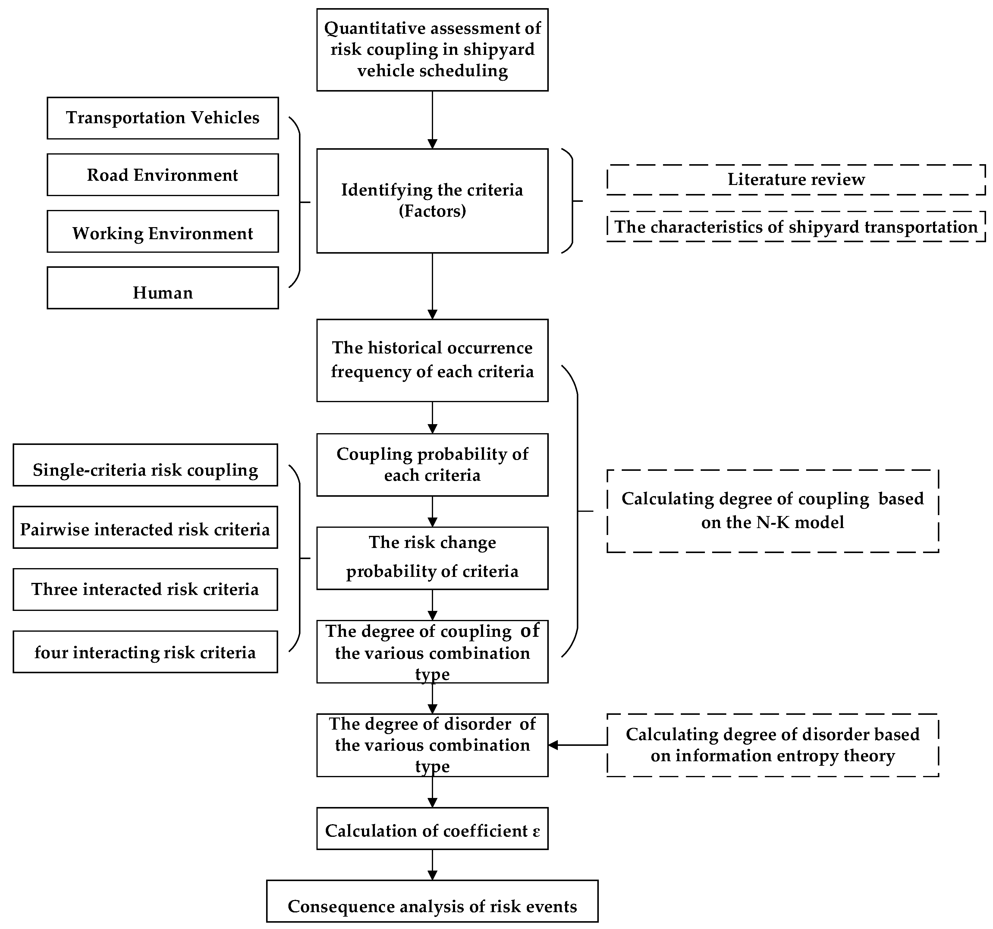
Figure 3.
Relationship between models.
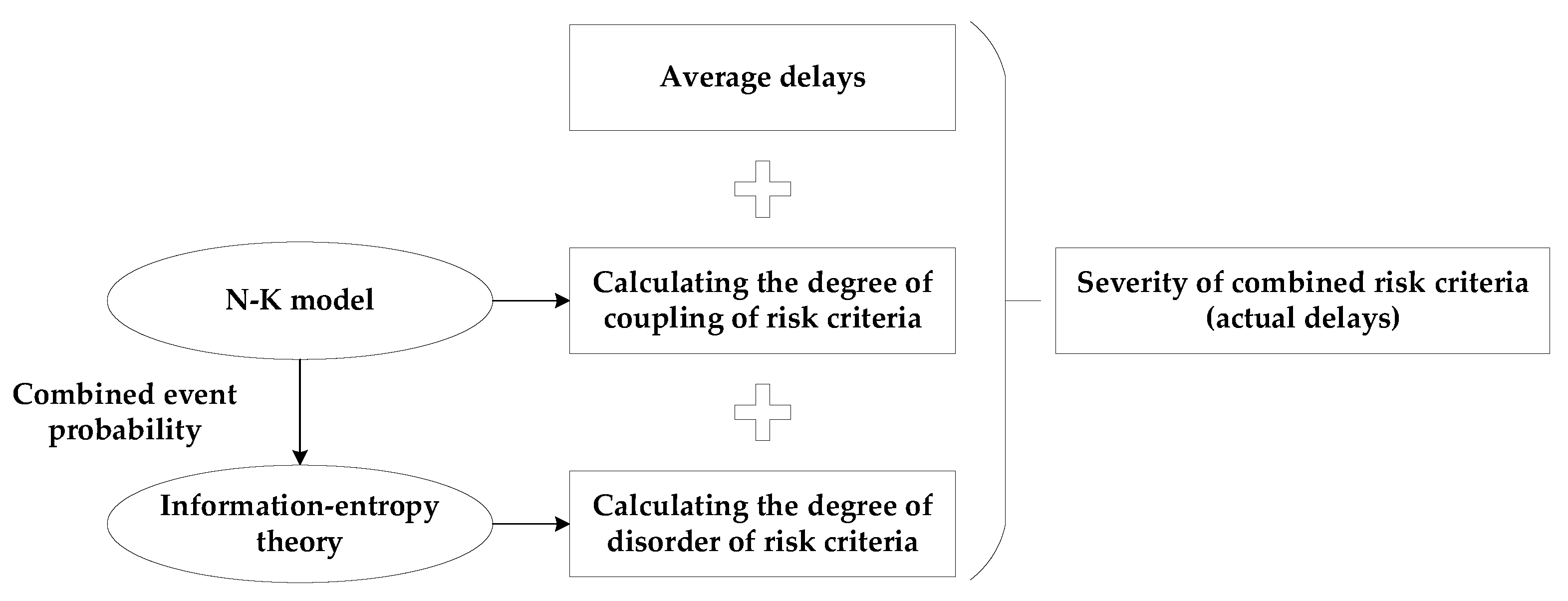
Figure 4.
The coupling mechanism of the VSS system.

Figure 5.
Values of different combinations.

Figure 6.
Summation of DD and DC for different interaction risk criteria.
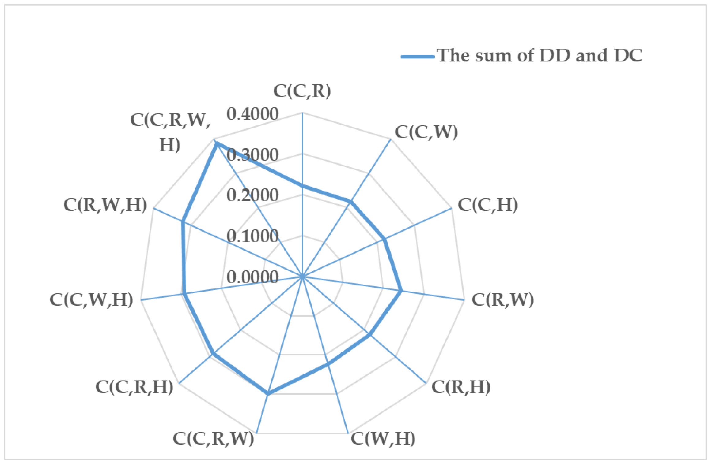
Figure 7.
Probability of combining risk criteria.
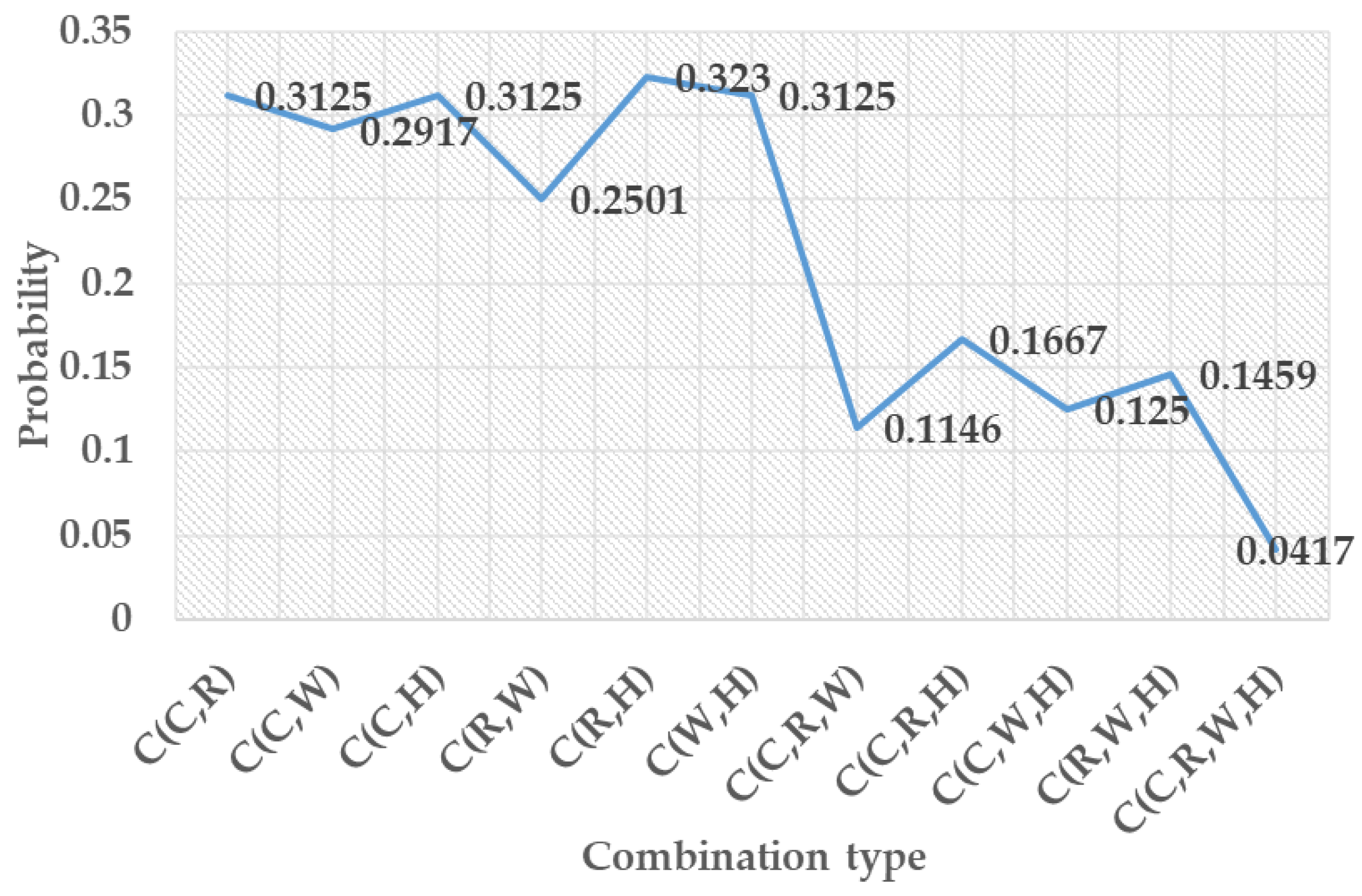
Figure 8.
Comparison of theoretical delays, Delay_Time_11, Delay_Time_12, and average delays.


Table 1.
Vehicle scheduling risk events according to Internet of Vehicles.
| No. | Incidents | Maintenance Cycle | Type | Delay Time (min) |
|---|---|---|---|---|
| 1 | Equipment failure | 9 h and 20 min | Maintenance | 31 |
| 2 | Maintenance | 1 days and 40 min | Maintenance | 32 |
| 3 | Oil pipe bursting | 23 h and 15 min | Oil leakage | 30 |
| 4 | Maintenance | 7 h and 52 min | Maintenance | 26 |
| 5 | Repairing water tanks | 5 days, 7 h and 45 min | Tank | 30 |
| 6 | High water temperature | 5 days, 23 h and 10 min | Tank | 35 |
| 7 | Loss of steering | 6 h and 45 min | Steering arm | 30 |
| 8 | Loss of steering | 2 days, 7 h and 32 min | Steering arm | 26 |
| 9 | Loss of steering | 7 h and 51 min | Steering arm | 28 |
| 10 | Maintenance of air conditioners | 59 min | Maintenance | 27 |
| 11 | Replacement parts | 18 h and 44 min | Maintenance | 28 |
| 12 | Flat tire | 12 h and 43 min | Steering arm | 29 |
| 13 | Oil leakage from cylinder | 3 days, 21 h and 11 min | Oil leakage | 32 |
| 14 | Maintenance | 5 h and 54 min | Maintenance | 32 |
| 15 | Oil leakage from cylinder | 2 days, 12 h and 2 min | Oil leakage | 34 |
| 16 | No signal | 9 h and 59 min | Network | 30 |
Table 2.
Road environment distribution risk events.
| No. | Incidents | Type | Delay Time (min) |
|---|---|---|---|
| 1 | Congestion caused by other vehicles | Other vehicles | 10 |
| 2 | Congestion caused by pedestrians | Pedestrians | 10 |
| 3 | Congestion caused by obstacles | Obstructions | 14 |
| 4 | Congestion caused by other vehicles | Other vehicles | 20 |
| 5 | Congestion caused by other vehicles | Other vehicles | 18 |
| 6 | Congestion caused by other vehicles | Other vehicles | 20 |
| 7 | Congestion caused by obstacles | Obstructions | 13 |
| 8 | Congestion caused by obstacles | Obstructions | 14 |
| 9 | Congestion caused by pedestrians | Pedestrians | 15 |
| 10 | Congestion caused by pedestrians | Pedestrians | 16 |
Table 3.
Working environment distribution risk events.
| No. | Incidents | Type | Delay Time (min) |
|---|---|---|---|
| 1 | Noise from the workplace | Noise | 4 |
| 2 | Drizzle | Bad weather | 10 |
| 3 | Heavy rain | Bad weather | 18 |
| 4 | Gale | Bad weather | 20 |
| 5 | Noise from the workplace | Noise | 7 |
| 6 | Heavy rain | Bad weather | 15 |
| 7 | frigid weather | Bad weather | 13 |
| 8 | Noise from the workplace | Noise | 5 |
| 9 | Hot weather | Bad weather | 13 |
| 10 | Gale | Bad weather | 16 |
Table 4.
The details of attributes of different risk criteria in VSS.
| Risk Criteria | Input | Output | Average Time (min) |
|---|---|---|---|
| Vehicle (C) | Maintenance | Vehicle needs replacement parts and maintenance | 30 |
| Oil leakage | Damage to the vehicle’s oil pipes or oil cylinders and other equipment, resulting in oil leakage from the vehicle | 30 | |
| Tank | The water temperature of the vehicle’s water tank is excessively high, or the water pump is abnormal | 30 | |
| Steering arm | The vehicle’s steering appears abnormal or its rocker arm breaks | 30 | |
| Tire | One or more of the tires on the vehicle are flat or runaway | 30 | |
| Network | There is no signal in the car network | 30 | |
| Road Environment (R) | Other vehicles | Other vehicles on the road impact scheduling | 15 |
| Obstructions | Space in the shipyard is limited and many blocks are placed on the roadside, which affects driving behavior | 15 | |
| Pedestrians | Congestion caused by pedestrians | 15 | |
| Working Environment (W) | Noise | There are various workshops in the shipyard, which generate significant noise and can affect drivers and pilots | 5 |
| Bad weather | This mainly refers to the impact of unfavorable weather, such as wind and rain, on traffic and staff | 15 | |
| Human (H) | Human behavior | There are many uncertainties in human behavior that can affect driving | 15 |
Table 5.
Delay distribution of risk factors.
| Risk Criteria | Factors | Number | Delay Ratio (Proportion of Delays Caused by the Factor) | |
|---|---|---|---|---|
| Vehicle (C) | Maintenance | 48 | 7.31% | 24.66% |
| Oil leakage | 22 | 3.35% | ||
| Tank | 6 | 0.91% | ||
| Steering arm | 43 | 6.54% | ||
| Tire | 32 | 4.87% | ||
| Network | 11 | 1.67% | ||
| Road Environment (R) | Other vehicles | 58 | 8.83% | 24.20% |
| Obstructions | 20 | 3.04% | ||
| Pedestrians | 81 | 12.33% | ||
| Working Environment (W) | Noise | 101 | 15.37% | 25.11% |
| Bad weather | 64 | 9.74% | ||
| Humans (H) | Human behavior | 171 | 26.03% | 26.03% |
Table 6.
Historical occurrence frequency Nc, r, w, h and coupling probability of each criterion Pc, r, w, h.
Table 6.
Historical occurrence frequency Nc, r, w, h and coupling probability of each criterion Pc, r, w, h.
| Frequency | = 0 | = 3 | = 15 |
| Probability | = 0 | = 0.0208 | = 0.0521 |
| Frequency | = 18 | = 12 | — |
| Probability | = 0.0625 | = 0.0417 | — |
| Frequency | = 21 | = 27 | = 18 |
| Probability | = 0.0729 | = 0.0938 | = 0.0625 |
| Frequency | = 9 | = 15 | = 24 |
| Probability | = 0.0313 | = 0.0521 | = 0.0833 |
| Frequency | = 21 | = 36 | = 24 |
| Probability | = 0.0729 | = 0.125 | = 0.0833 |
| Frequency | = 30 | = 12 | — |
| Probability | = 0.1042 | = 0.0417 | — |
Table 7.
Risk-change probabilities for each single-criteria risk coupling.
| Type | Pc=0 | Pc=1 | Pr=0 | Pr=1 | Pw=0 | Pw=1 | Ph=0 | Ph=1 |
| Probability | 0.4272 | 0.5729 | 0.4479 | 0.5522 | 0.4271 | 0.573 | 0.4063 | 0.5938 |
Table 8.
Risk-change probabilities of the pairwise-interacting risk criteria (PIRC).
| Type | Pc=0,r=0 | Pc=0,r=1 | Pc=1,r=0 | Pc=1,r=1 | Pr=0,w=0 | Pr=1,w=0 | Pr=0,w=1 | Pr=1,w=1 |
| Probability | 0.1875 | 0.2397 | 0.2604 | 0.3125 | 0.125 | 0.3021 | 0.3229 | 0.2501 |
| Type | Pr=0,h=0 | Pr=1,h=0 | Pr=0,h=1 | Pr=1,h=1 | Pw=0,h=0 | Pw=1,h=0 | Pw=0,h=1 | Pw=1,h=1 |
| Probability | 0.1771 | 0.2292 | 0.2708 | 0.323 | 0.1458 | 0.2605 | 0.2813 | 0.3125 |
| Type | Pc=1,h=0 | Pc=1,h=1 | Pc=0,h=1 | Pc=0,h=0 | Pc=1,w=0 | Pc=1,w=1 | Pc=0,w=0 | Pc=0,w=1 |
| Probability | 0.2604 | 0.3125 | 0.2813 | 0.1459 | 0.2812 | 0.2917 | 0.1459 | 0.2813 |
Table 9.
Risk-change probabilities of three-interacting risk criteria (TIRC).
| Type | Pc=0,r=0,w=0 | Pc=1,r=0,w=0 | Pc=0,r=1,w=0 | Pc=0,r=0,w=1 | Pc=1,r=1,w=0 | Pc=1,r=0,w=1 | Pc=0,r=1,w=1 |
| Probability | 0.0417 | 0.0833 | 0.1042 | 0.1458 | 0.1979 | 0.1771 | 0.1355 |
| Type | Pc=1,r=1,w=1 | Pr=0,w=0,h=0 | Pr=1,w=0,h=0 | Pr=0,w=1,h=0 | Pr=0,w=0,h=1 | Pc=0,r=0,h=0 | Pc=1,r=0,h=0 |
| Probability | 0.1146 | 0.0208 | 0.125 | 0.1563 | 0.1042 | 0.0625 | 0.1146 |
| Type | Pc=0,r=1,h=0 | Pc=0,r=0,h=1 | Pc=1,r=1,h=0 | Pc=1,r=0,h=1 | Pc=0,r=1,h=1 | Pc=1,r=1,h=1 | Pc=0,w=0,h=0 |
| Probability | 0.0834 | 0.125 | 0.1458 | 0.1458 | 0.1563 | 0.1667 | 0.0521 |
| Type | Pc=1,w=0,h=0 | Pc=0,w=1,h=0 | Pc=0,w=0,h=1 | Pc=1,w=1,h=0 | Pc=1,w=0,h=1 | Pc=0,w=1,h=1 | Pc=1,w=1,h=1 |
| Probability | 0.0937 | 0.0938 | 0.0938 | 0.1667 | 0.1875 | 0.1875 | 0.125 |
| Type | Pr=1,w=1,h=0 | Pr=1,w=0,h=1 | Pr=0,w=1,h=1 | Pr=1,w=1,h=1 | |||
| Probability | 0.1042 | 0.1771 | 0.1666 | 0.1459 |
Table 10.
Risk-change probabilities of four-interacting risk criteria (FIRC).
| Type | Pc=0,r=0,w=0,h=0 | Pc=1,r=0,w=0,h=0 | Pc=0,r=1,w=0,h=0 | Pc=0,r=0,w=1,h=0 | Pc=0,r=0,w=0,h=1 |
| Probability | 0 | 0.0208 | 0.0521 | 0.0625 | 0.0417 |
| Type | Pc=1,r=1,w=0,h=0 | Pc=0,r=1,w=1,h=0 | Pc=0,r=1,w=0,h=1 | Pc=0,r=0,w=1,h=1 | Pc=1,r=1,w=1,h=0 |
| Probability | 0.0729 | 0.0313 | 0.0521 | 0.0833 | 0.0729 |
| Type | Pc=1,r=1,w=0,h=1 | Pc=1,r=0,w=1,h=1 | Pc=1,r=0,w=1,h=0 | Pc=1,r=0,w=0,h=1 | Pc=0,r=1,w=1,h=1 |
| Probability | 0.125 | 0.0833 | 0.0938 | 0.0625 | 0.1042 |
| Type | Pc=1,r=1,w=1,h=1 | ||||
| Probability | 0.0417 |
Table 11.
Values of the various combination types.
| Combination Type | C(C, R) | C(C, W) | C(C, H) | C(R, W) | C(R, H) | C(W, H) |
| C(x) | 0.003955 | 0.001613 | 0.009267 | 0.053291 | 0.000142 | 0.014472 |
| H(x) | 0.4389 | 0.4329 | 0.4309 | 0.4315 | 0.4353 | 0.4309 |
| Sum | 0.2214 | 0.2173 | 0.2201 | 0.2424 | 0.2177 | 0.2227 |
| Combination Type | C(C, R, W) | C(C, R, H) | C(C, W, H) | C(R, W, H) | C(C, R, W, H) | |
| C(x) | 0.072486 | 0.00968 | 0.036161 | 0.083253 | 0.153196 | |
| H(x) | 0.5274 | 0.5686 | 0.548 | 0.5609 | 0.6192 | |
| Sum | 0.2999 | 0.2891 | 0.2921 | 0.3221 | 0.3862 | |
Table 12.
Actual delay time for each combination of events for July 2022 to October 2022.
| Combination Type | T (C, R) | T (C, W) | T (C, H) | T (R, W) | T (R, H) | T (W, H) |
| Delay_Time_1 | 45 | 47 | 55 | 32 | 36 | 33 |
| Delay_Time_2 | 47 | 52 | 45 | 38 | 34 | 35 |
| Delay_Time_3 | 51 | 53 | 55 | 32 | 33 | 32 |
| Delay_Time_4 | 55 | 54 | 50 | 35 | 34 | 38 |
| Delay_Time_5 | 52 | 49 | 50 | 36 | 33 | 38 |
| Delay Time_6 | 50 | 46 | 50 | 37 | 35 | 32 |
| Delay_Time_7 | 48 | 47 | 55 | 35 | 34 | 38 |
| Delay_Time_8 | 47 | 55 | 47 | 32 | 35 | 36 |
| Delay_Time_9 | 50 | 52 | 45 | 36 | 36 | 36 |
| Delay_Time_10 | 55 | 48 | 50 | 38 | 37 | 32 |
| Delay_Time_11 | 52 | 48 | 51 | 33 | 38 | 36 |
| Delay_Time_12 | 48 | 49 | 47 | 36 | 35 | 34 |
| Combination Type | T (C, R, W) | T (C, R, H) | T (C, W, H) | T (R, W, H) | T (C, R, W, H) | |
| Delay_Time_1 | 60 | 58 | 69 | 49 | 103 | |
| Delay_Time_2 | 68 | 70 | 65 | 50 | 99 | |
| Delay_Time_3 | 74 | 56 | 60 | 52 | 84 | |
| Delay_Time_4 | 67 | 59 | 70 | 58 | 87 | |
| Delay_Time_5 | 58 | 61 | 75 | 65 | 103 | |
| Delay Time_6 | 70 | 59 | 75 | 73 | 77 | |
| Delay_Time_7 | 59 | 70 | 67 | 57 | 83 | |
| Delay_Time_8 | 64 | 63 | 66 | 71 | 79 | |
| Delay_Time_9 | 71 | 75 | 57 | 73 | 100 | |
| Delay_Time_10 | 64 | 70 | 61 | 57 | 75 | |
| Delay_Time_11 | 68 | 72 | 57 | 46 | 102 | |
| Delay_Time_12 | 57 | 67 | 58 | 69 | 88 | |
Table 13.
Values of for different groups.
| Value | 0.7404 | 0.7657 | 0.7185 | 0.7576 | 0.7912 | 0.7489 | 0.7326 | 0.7324 | 0.8089 | 0.7156 |
Table 14.
Theoretical delays for each combination of criteria.
| Combination Type | T (C, R) | T (C, W) | T (C, H) | T (R, W) | T (R, H) | T (W, H) |
| Delays | 48.63 | 48.42 | 48.56 | 34.78 | 33.91 | 34.09 |
| Combination Type | T (C, R, W) | T (C, R, H) | T (C, W, H) | T (R, W, H) | T(C, R, W, H) | |
| Delays | 68.32 | 67.62 | 67.81 | 53.66 | 90.99 | |
Disclaimer/Publisher’s Note: The statements, opinions and data contained in all publications are solely those of the individual author(s) and contributor(s) and not of MDPI and/or the editor(s). MDPI and/or the editor(s) disclaim responsibility for any injury to people or property resulting from any ideas, methods, instructions or products referred to in the content. |
© 2024 by the authors. Licensee MDPI, Basel, Switzerland. This article is an open access article distributed under the terms and conditions of the Creative Commons Attribution (CC BY) license (https://creativecommons.org/licenses/by/4.0/).
Share and Cite
MDPI and ACS Style
Wang, N.; Yin, J.; Khan, R.U. Risk Coupling Assessment of Vehicle Scheduling for Shipyard in a Complicated Road Environment. J. Mar. Sci. Eng. 2024, 12, 685. https://doi.org/10.3390/jmse12040685
AMA Style
Wang N, Yin J, Khan RU. Risk Coupling Assessment of Vehicle Scheduling for Shipyard in a Complicated Road Environment. Journal of Marine Science and Engineering. 2024; 12(4):685. https://doi.org/10.3390/jmse12040685
Chicago/Turabian StyleWang, Ningfei, Jingbo Yin, and Rafi Ullah Khan. 2024. "Risk Coupling Assessment of Vehicle Scheduling for Shipyard in a Complicated Road Environment" Journal of Marine Science and Engineering 12, no. 4: 685. https://doi.org/10.3390/jmse12040685
Note that from the first issue of 2016, this journal uses article numbers instead of page numbers. See further details here.