
Distributed Formation–Containment Tracking Control for Multi-Hovercraft Systems with Compound Perturbations
College of Intelligent Systems Science and Engineering, Harbin Engineering University, Harbin 150006, China
*
Author to whom correspondence should be addressed.
J. Mar. Sci. Eng. 2024, 12(5), 694; https://doi.org/10.3390/jmse12050694
Submission received: 25 March 2024
/
Revised: 18 April 2024
/
Accepted: 19 April 2024
/
Published: 23 April 2024
(This article belongs to the Special Issue Unmanned Marine Vehicles: Perception, Planning, Control and Swarm)
Abstract
:Aiming at the problem of hovercraft formation–containment control with compound perturbations including model uncertainties and ocean disturbances, a distributed control algorithm for underactuated hovercraft formation–containment is proposed by combining adaptive linear extended state observer (ALESO) and radial basis function neural network (RBFNN). Firstly, ALESO and RBFNN are designed to estimate the ocean disturbances and model uncertainties, respectively, for dynamic compensation in the controller. Then, the auxiliary variables are introduced into the formation error function, and the lateral and longitudinal error stabilization is transformed into the design of longitudinal force and rotational torque by using the skew-symmetric matrix transformation, which solves the lateral underactuated problem of the hovercraft. Finally, the uniform ultimate boundedness of formation–containment cooperative errors is proved by the Lyapunov stability theory. Digital simulation verifies the effectiveness of the proposed method.
1. Introduction
As a high-performance vessel, a hovercraft can travel at high speed on particular surfaces, such as ice, swamps, beaches, grass, etc., which cannot be achieved by conventional surface vessels [1,2]. Currently, the research on hovercraft mainly focuses on the heading, rotation rate, and trajectory tracking control problem of a single hovercraft under constraint conditions [3,4,5,6,7]. However, a single hovercraft may face issues such as insufficient personnel and carrying resources when the task is more complex. For specific complex tasks, there is a need for more intelligent multi-hovercraft systems that can encompass a broader range of practical engineering task requirements. The multi-hovercraft can complete the assigned task through cooperation and collaboration, which can significantly improve the efficiency of task completion.
With the in-depth study of multi-agent cooperative control problems, many related research branches have emerged, such as formation control [8,9,10,11], containment control [12,13,14], etc. Based on the leader-follower idea, the mathematical model of the formation is given in [15]; that is, all leaders will track the time-varying trajectory obtained by the decomposition of the desired formation configuration, and the followers are distributed to the convex hull formed by the leaders. Based on this model, this paper designs a formation–containment configuration model for multi-hovercraft systems to meet some specific mission requirements of multi-hovercraft systems, such as formation escort operations. The advantage of the multi-hovercraft formation–containment configuration is that some of the vessels in the multi-hovercraft system with better performance and equipment can be considered as the leader vessels, and the rest as the follower vessels, and a control strategy can be adapted to converge the follower into the convex hull formed by the leaders. In the process of this cooperative control task, the followers are only responsible for the transportation task, while the leaders with better performance are not only responsible for the transportation task but also responsible for monitoring the surrounding environment, eliminating potential security risks and other tasks while protecting the followers of the inner layer [16,17,18].
The hull structure and cushion navigation characteristics of the hovercraft are different from those of the conventional surface vessel, which causes it to have uncertainties such as parameter uncertainties, modeling errors, and other unknown ocean disturbances [19]. At the same time, the hovercraft is a typical underactuated vessel due to the lack of a lateral propulsion mechanism. How to reduce the influence of uncertainties on hovercraft and improve the anti-interference ability of hovercraft is a difficult problem. For complex model modeling problems, scholars have proposed many solutions, such as extended state observer-based control [20,21], model-free adaptive control [22], neural network control [3,23], and data-driven control [24]. The extended state observer (ESO) proposed by J.H. in his pioneering work [25] not only has the ability of state observation but also can estimate the generalized disturbances between the controlled object and the controlled object model in real time. In [20], an adaptive ESO is designed to estimate the unmeasurable linear velocity, angular velocity, and unknown external disturbances. The slowly varying environmental disturbances and model uncertainties are treated separately, and experiments prove the method’s effectiveness. Since a neural network (NN) can approximate any nonlinear functions, the adaptive controller based on a neural network has been widely used in objects with model uncertainties and unknown disturbances [3]. Reference [24] developed a model-free fuzzy control law based on a data-driven fuzzy predictor, which simultaneously learns unknown control gains and uncertain dynamics. Aiming at the underactuated problem of hovercraft, the literature [26] transformed the lateral thrust design into the yaw moment under underactuated by introducing an auxiliary variable, which solved the underactuated problem of a three-degree-of-freedom (3-DOF) surface vessel. In reference [17], the collision avoidance problem in formation–containment tracking control of multiple USVs with limited speed and driving force is studied, but the uncertainty of the model is not considered. In [16,18], the time-varying formation–containment problem of multiple unmanned underwater vehicle systems in three-dimensional space is studied and an extended state observer is designed to estimate the external disturbance and unknown nonlinearity in real time, but the underactuated problem of the system is not considered.
Inspired by the above scheme, this paper studies the formation–containment control problem of underactuated hovercraft with ocean disturbances and model uncertainties. The main contributions of this paper can be briefly summarized as follows:
- Compared with the literature [27], this paper expands the formation–containment motion to the cooperative mission of 4-DOF hovercraft that considers compound uncertainties and underactuated problems. Furthermore, the asymptotic stability of the controller is proved by Lyapunov’s method. This layered structure allows for more complex and flexible tasks and provides greater adaptability to the complex sea operations of hovercraft.
- By introducing an auxiliary variable in the cooperative error, the underactuated problem of the hovercraft is solved. Compared with the literature [7], multiple derivations of the virtual control law are avoided, thus reducing the excessive differential terms in the yaw direction control law. Compared with reference [18], a novel scheme is designed to solve the underactuated problem in the formation–containment controller design process.
- A novel ALESO is combined with RBFNN to estimate the unknown ocean disturbances and model uncertainties of hovercraft. Compared with reference [20], the ALESO relaxes the restriction on the change rate of disturbances. By adding a linear adaptive factor to the adaptive update law, it is easy to prove that all the closed-loop signals of the whole system are boundedly stable.
The remainder of this paper is organized as follows: Section 2 presents the mathematical models and preliminary knowledge. In Section 3, the formation–containment controller is proposed. Cooperative stability analysis is presented in Section 4. Furthermore, a simulation example is given in Section 5. Finally, Section 6 presents some conclusions.
2. Mathematical Models and Preliminary Knowledge
2.1. Mathematical Models
Consider a multi-hovercraft system consisting of leaders, followers, and a virtual leader, where . The virtual leader number is defined as 0, the leader number is defined as , and the follower number is defined . The reference system diagram of the hovercraft is shown in Figure 1. The 4-DOF kinematic model of the th hovercraft is as follows
where , represents the position and attitude information of the th hovercraft; represents the velocity information of the th hovercraft; denotes the coordinate transformation matrix of the th hovercraft, where , . Suppose that the roll angle .
The dynamic model of the th hovercraft is as follows
where , and represent the mass and moment of inertia of the hovercraft, respectively. , , and represent the total resistance of the model in each degree of freedom direction [3], and represent the longitudinal and yaw direction control input, respectively. denotes the impact of model uncertainty, represents the impact of ocean disturbance and denotes compound perturbations.
Assumption 1.
The model uncertainty term and its first time derivative
are bounded. Moreover, ocean disturbance term and its first time derivative are bounded as well.
The resultant velocity of the th hovercraft is defined as , , . Then, (1) can be rewritten as
where , .
2.2. Preliminary Knowledge
The directed topology graph is used to describe the communication relationship between hovercrafts, where the node set represents the set of all hovercrafts, and the edge set represents the set of edges of the communication relationship between hovercrafts. Edge indicates that the th hovercraft can obtain the information of the th hovercraft, where the th hovercraft refers to the adjacent hovercraft of the th hovercraft. An adjacency matrix is defined to describe the communication relationship between nodes, which is expressed as . If , then ; otherwise, . In addition, the Laplacian matrix is defined as , which can be expressed as in blocks, where denotes the communication relationship between the leaders, and denotes the communication relationship between the followers and the leaders; denotes the communication relationship between the followers. In addition, define ; if the th leader can obtain the information of the virtual leader, then , . Otherwise, , and define matrix .
Assumption 2.
[27]. There is at least one path from the virtual leader to each leader. In addition, the leaders have at least one path to each follower.
Lemma 1.
[27]. Under the condition of Assumption 2, all eigenvalues of matrix have positive real parts, and each element of is non-negative and the sum of each row of is 1.
2.3. Control Objective
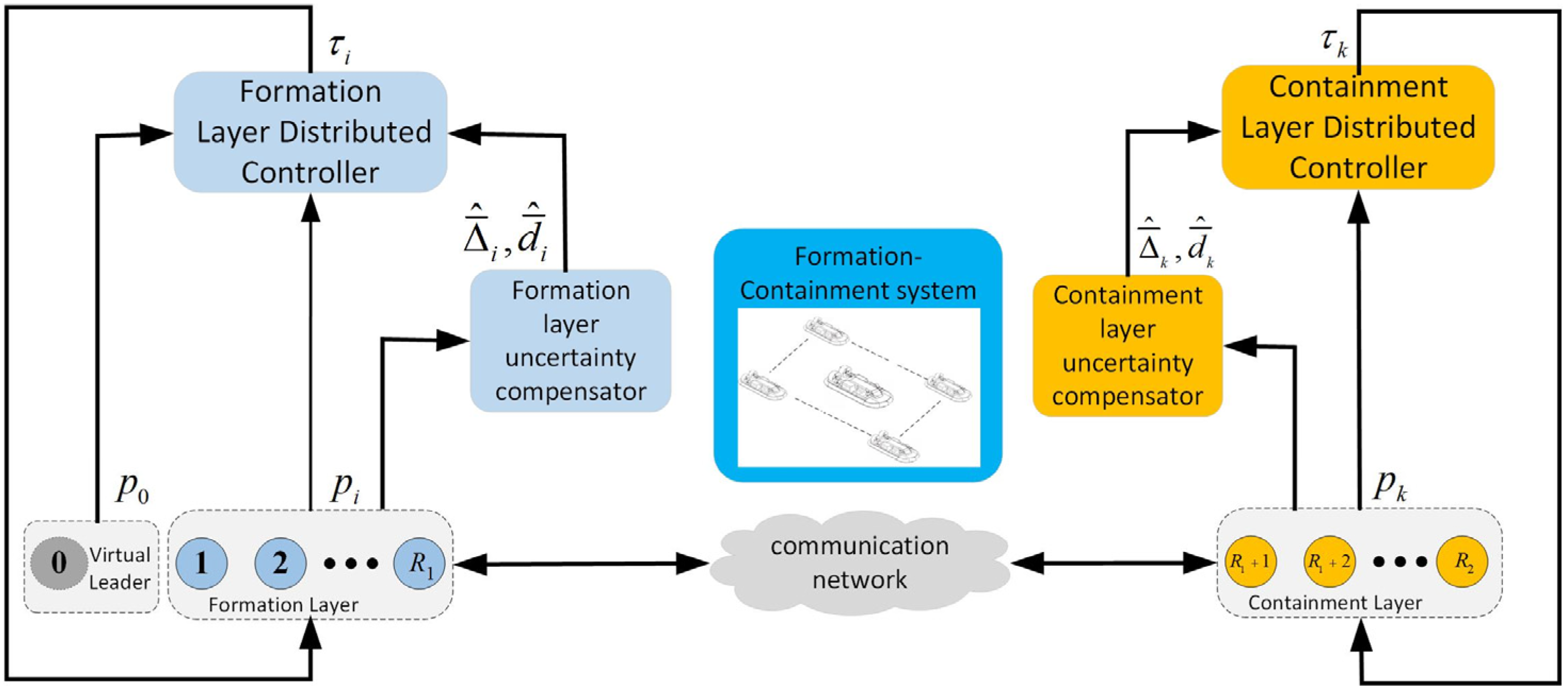
In this paper, a distributed formation–containment control scheme for 4-DOF underactuated hovercraft under the condition of ocean disturbances and model uncertainties is proposed. The block diagram of the control system is shown in Figure 2. The control objectives are as follows:
- (1)
- In the formation layer, the control scheme is used to make the formula , hold, in which and represent the position information of the th leader and the virtual leader, respectively. represents the expected position deviation of the leader hovercraft relative to the virtual leader hovercraft, is a small constant, and the leaders in the multi-hovercraft system realize formation tracking.
- (2)
- In the containment layer, the control scheme is used to make , hold, where the non-negative constant satisfies , is the position information of the th hovercraft, and is a small constant, and the followers in the multi-hovercraft system realize the containment control.
Figure 2.
The framework of control system.

3. Formation–Containment System Controller Design
This section proposes a formation tracking control scheme for the leaders and a containment control scheme for the followers in the backstepping framework.
3.1. Formation Layer Controller Design
In order to track the virtual leader, a formation control scheme is designed for the leader in the formation layer under the condition of ocean disturbances and model uncertainties.
Firstly, the distributed cooperative error of the formation layer is defined as follows
where , . and represent the position information of the leader , , respectively. represent the position information of the virtual leader. represents the expected position deviation of the leader relative to the leader . represents the expected position deviation of the leader relative to the virtual leader.
The time derivative of (4) can be written as
where , .
Considering that there is no thruster on the side of the hovercraft, an auxiliary variable is introduced to transform the lateral thrust design into the yaw moment design to solve the hovercraft’s underactuated problem [28]. The cooperative error is redefined as follows
where , is a positive number. According to (5) and (6), the dynamic equation of can be expressed as follows
where , , , .
To stabilize the dynamic process of (7), the virtual control law of the formation layer is designed as follows
where is a diagonal gain matrix. Substituting (8) into (7), we have
where , is the output of the linear tracking differentiator, which will be introduced later; is the dynamic tracking error.
According to (3), we have , . Combined with (2), we have
Taking the time derivative of and combined with (10), we have
where , , , , , , is the output value of the differentiator. The total impact of and can be expressed as .
The following linear differentiator is designed to estimate the differential value of the virtual control law.
where is the estimated value of , and is the diagonal gain matrix. According to the convergence analysis of the linear differentiator in [29], it is known that the output error , of the differentiator can converge to any small bounded domain.
Since the ocean disturbance term in (11) is unknown, an adaptive extended state observer (ALESO) is designed to estimate it.
The extended state vector is defined as , and unknown ocean disturbance is defined as an extended state variable. According to (11), we have
where , , .
Inspired by [20], the ALESO in this paper is designed as follows
where is the estimation of , , where and is the observer estimation error. The observer gain is designed as , where represent diagonal gain matrices.
where , , and adaptive variable will be introduced later. Assume that satisfies the following matching condition.
where , , . The time-varying matrix is defined as follows
where , .
Based on Assumption 1, it is easy to know that is bounded, so is bounded. Assume that has an unknown upper bound that satisfies the inequality relation . The adaptive update rate of is designed as follows
where , , define , adaptive estimation error . Subtract (14) from (13), we can obtain
where is Hurwitz. There is a positive definite symmetric matrix satisfying
In order to prove the convergence of the observer estimation error, the following Lyapunov function is selected
The time derivative of can be written as
Substituting (15), (16), (18) and (20) into (22), we have
where , . Solving (23), we have, when , the estimation error of the observer can converge to a bounded domain, and the size of the bounded domain can be adjusted by reasonably selecting parameters.
Next, to deal with the model uncertainties in (11), the RBFNN is designed to approximate , and the projection operator is introduced to limit the upper and lower bounds of the weights of the adaptive neural network. The input-output RBFNN algorithm is designed as follows
where is the ideal weight matrix, which satisfies , , is the network approximation error, basis function , where , respects the central position and width of the th neuron, respectively. is network input. The output of RBFNN is
where is the estimation, letting . The adaptive weight matrix update law of the neural network is designed as follows:
The definition and properties of the projection operator can be found in reference [30].
Based on the output values of differentiator, ALESO and RBFNN, the distributed cooperative anti-interference control law of multi-hovercraft is designed as follows
where is a diagonal gain matrix.
Choosing a Lyapunov function candidate as
whose time derivative alone (9), (23), (24), (25), (26) and (27), we have
where , .
According to (29), we have . When , the system error can converge to a bounded domain, and the size of the bounded domain can be adjusted by reasonably selecting the parameters.
3.2. Containment Layer Controller Design
Next, a control scheme is designed for the following hovercraft . The definition of the containment layer error function is as follows
where , , and . , and represent the position information of the followers , and the leader , respectively.
Taking the time derivative of (30) along (2), we have
where . The auxiliary variable is introduced to solve the underactuated problem of the hovercraft, and the tracking error is redefined as follows
where , is a positive constant whose time derivative (32) along (31) satisfies
where , , , .
In order to stabilize (33), the distributed virtual control law of the underactuated hovercraft with a containment layer is designed as follows
where is the diagonal gain matrix. Substituting (34) into (33), one has
where , is the output of the tracking differentiator, which will be introduced later. is dynamic tracking error.
Taking the time derivative of , it follows that
where , , , , , , is the output value of the differentiator, and the design form of the differentiator is completely consistent with (12). The total impact of and can be expressed as .
Next, ALESO and RBFNN are introduced to estimate the unknown ocean disturbance and model uncertainties in (36), respectively. The design form of ALESO and RBFNN is completely consistent with the formation layer, and the design process is omitted here.
The distributed cooperative control law of the multi-hovercraft with a containment layer is designed as follows
where is a diagonal gain matrix.
Referring to the formation layer Lyapunov function form, the containment layer Lyapunov function can be finally organized into the following form
where , .
4. Stability Analysis
Theorem 1.
Consider a multi-hovercraft system consisting of leaders and followers and satisfying the relevant assumptions, as expressed in (3). Then, the control law (27), (37) and the virtual control law Equations (8) and (34) proposed in this paper can make the multi-hovercraft system achieve formation–containment control, and the formation tracking error and the containment tracking error can converge to a bounded domain.
Proof of Theorem 1.
Consider the following Lyapunov function
The time derivative of (39) can be written as
where , .
According to (40), we have
Then, we have
Equation (41) implies that is bounded, and the error signals , , , , , , , and are bounded. Combining (6), (32) shows that the error , is bounded. Therefore, the boundedness of all signals in the multi-hovercraft system is guaranteed.
Define , , , , and .
According to (42), we have
where .
Substituting (6) into (33), we have
The formation tracking error of the leaders can be defined as . Then, the formation tracking error of all leaders can be defined as . According to (4), we have , then the formation tracking error satisfies
where is the minimum singular value of matrix .
Define , , , and the following hovercraft containment error is defined as . According to Lemma 1, the sum of each row of is 1, and the containment error of all following hovercraft is written as . According to (42), one has
According to (30), we have
Then, the containment error satisfies
where is the minimum singular value of matrix .
By adjusting the parameters reasonably, the tracking error can be adjusted to the bounded domain, that is, , . This completes the proof. □
5. Simulation
In this section, simulation results are provided to illustrate the efficacy of the proposed multi-hovercraft formation–containment control scheme. The communication topology between the multi-hovercraft system is shown in Figure 3, which includes the virtual leader (Hovercraft #0), three leaders (Hovercraft #1–Hovercraft #3) in the formation layer, and two follower (Hovercraft #4–Hovercraft#5) in the containment layer.
For detailed information on the main parameters of the hovercraft used in the simulation, please refer to [3]. The formation structure vector information is set as , , , auxiliary variables are set as . The initial state of the ALESO, linear differentiator and RBFNN is set as zero. The initial state of the multi-hovercraft system is designed as , , , , , , , , , , , .
The desired trajectory generated by a virtual leader consists of two straight lines and a circular arc [4]. , , , , , the desired trajectory which is shown in Figure 4 is given by
where
The parameters of the control are designed as , , , , , , , , , . The parameters of ALESO are set as , , , . The parameters of the differentiator are set as . The parameters of RBFNN are set as , , , . The model uncertainties were modeled using the following functional form: . The effect of ocean disturbances on the system is modeled in the following functional form [4]:
where , , , ,, and are wind coefficients, and are wind torque coefficients, is the density of air, and are the frontal and lateral projected areas, and are the height of the hovercraft, denotes pulsating wind speed, is pulsating wind frequency, denotes wind spectrum. is the height above water, is the average wind speed, .
where , , , , , is the density of water, denotes gravitational acceleration, is wave frequency, denotes wave spectrum. is the height of water.
The simulation results are illustrated in Figure 4, Figure 5, Figure 6 and Figure 7. Figure 4 illustrates the trajectories of three leaders (Hovercraft #1–Hovercraft #3) and two followers (Hovercraft #4–Hovercraft #5) under compound perturbation conditions. At the beginning of the simulation, Hovercraft #4 and Hovercraft #5 are located outside the convex envelope shaped by Hovercraft #1–Hovercraft #3. By using the proposed formation–containment scheme, Hovercraft #4 and Hovercraft #5 can be successfully guided into the convex envelope formed by the leaders. The multi-hovercraft system distributed cooperative errors, formation tracking error of Hovercraft #1–Hovercraft #3, and containment tracking error of Hovercraft #4 and Hovercraft #5 are plotted in Figure 5 and Figure 6, respectively. From Figure 5 and Figure 6, it can be seen that the coordination error, formation tracking control error, and containment tracking control error can converge to the bounded domain. In order to show the superiority of the algorithm in this paper, the control algorithm provided in the literature [17] is compared with this paper in the simulation. The contrast effect diagram is shown in Figure 6. Method 1 represents the control scheme of this paper, and method 2 represents the control scheme of reference [17]. It can be seen from Figure 6 that the method designed in this paper makes the followers have higher tracking accuracy. When and , the tracking errors fluctuate due to the change in the rotation rate, but the errors converge quickly. Figure 7 represents the total estimated effect of ALESO on the unknown ocean disturbances and RBFNN on the model uncertainties. From Figure 7, it can be observed that ALESO and RBFNN achieve a good estimation effect.
![Jmse 12 00694 g004]()
![Jmse 12 00694 g005]()
![Jmse 12 00694 g006]()
![Jmse 12 00694 g007]()
Figure 4.
Multi–hovercraft formation–containment movements trajectories.

Figure 5.
Distributed cooperative errors of multi-hovercraft system.

Figure 6.
Formation tracking errors and containment tracking errors.

Figure 7.
Compound perturbations and its estimated value.

The velocity curve of the hovercraft is shown in Figure 8. It is worth noting that the heeling velocity of the hovercraft fluctuates obviously. Due to the lack of control torque, the heeling angle and angular velocity cannot be limited. Future work should consider reducing the fluctuation of the heeling angle. The control force and torque of the hovercraft are shown in Figure 9. In the initial phase, the response curve of control force and torque fluctuates largely due to the large formation tracking control error and containment tracking control error at the beginning. When the multi-hovercraft system reaches a stable state, the control torque value fluctuates within a small range.
6. Conclusions
This paper studies the formation–containment control problem of multi-hovercraft systems under compound uncertainties. The designed ALESO and RBFNN effectively compensate for unknown ocean disturbances and model uncertainties of the multi-hovercraft system. The stability of the multi-hovercraft system is analyzed using Lyapunov’s stability theory, and it is concluded that the tracking errors can converge to a bounded domain. Finally, simulation results show that the scheme proposed in this paper can achieve multi-hovercraft formation–containment control with small distributed cooperative errors under compound perturbations. In future research, we will focus on model-free control schemes and connectivity maintenance of the multi-hovercraft system.
Author Contributions
Z.F., literature search, graphing, and writing; Y.X., methodology, study design, and writing; M.F. methodology, study design, and funding acquisition. All authors have read and agreed to the published version of the manuscript.
Funding
This research were funded by the National Natural Science Foundation of China (Grant Numbers 52071112) and National Key Basic Strengthen Research Foundation of China (No: JCJQ-ZD-186-00).
Data Availability Statement
The original data contributions presented in the study are included in the article; further inquiries can be directed to the corresponding authors.
Conflicts of Interest
The authors declare no conflicts of interest.
References
- Fu, H. Analysis and Consideration on Safety of All-lift Hovercraft. Ship Boat 2008, 19, 1–3. [Google Scholar]
- Yun, L.; Wu, C. High-performance ships for the 21st century. Ship Ocean Eng. 1997; 3–5+7–8+10–12. [Google Scholar]
- Fu, M.; Gao, S.; Wang, C.; Li, M. Design of driver assistance system for air cushion vehicle with uncertainty based on model knowledge neural network. Ocean Eng. 2019, 172, 296–307. [Google Scholar] [CrossRef]
- Fu, M.; Dong, L.; Xu, Y.; Dan, B. A novel asymmetrical integral barrier Lyapunov function-based trajectory tracking control for hovercraft with multiple constraints. Ocean Eng. 2022, 263, 112132. [Google Scholar] [CrossRef]
- Fu, M.; Zhang, T.; Ding, F.; Wang, D. Safety-guaranteed adaptive neural motion control for a hovercraft with multiple constraints. Ocean Eng. 2021, 220, 108401. [Google Scholar] [CrossRef]
- Morales, R.; Sira-Ramirez, H.; Somolinos, J.A. Linear active disturbance rejection control of the hovercraft vessel model. Ocean Eng. 2015, 96, 100–108. [Google Scholar] [CrossRef]
- Fu, M.; Zhang, T.; Ding, F. Adaptive finite-time PI sliding mode trajectory tracking control for underactuated hovercraft with drift angle constraint. IEEE Access 2019, 7, 184885–184895. [Google Scholar] [CrossRef]
- Chen, L.; Mei, J.; Li, C.; Ma, G. Distributed Leader-Follower Affine Formation Maneuver Control for High-Order Multiagent Systems. IEEE Trans. Autom. Control 2020, 65, 4941–4948. [Google Scholar] [CrossRef]
- Dong, X.; Yu, B.; Shi, Z.; Zhong, Y. Time-Varying Formation Control for Unmanned Aerial Vehicles: Theories and Applications. IEEE Trans. Control Syst. Technol. 2015, 23, 340–348. [Google Scholar] [CrossRef]
- Hu, J.; Bhowmick, P.; Lanzon, A. Distributed Adaptive Time-Varying Group Formation Tracking for Multiagent Systems with Multiple Leaders on Directed Graphs. IEEE Trans. Control Netw. Syst. 2020, 7, 140–150. [Google Scholar] [CrossRef]
- Lin, A.; Jiang, D.; Zeng, J.-P. Underactuated Ship Formation Control with Input Saturation. Acta Autom. Sin. 2018, 44, 1496–1504. [Google Scholar]
- Gu, N.; Peng, Z.; Wang, D.; Zhang, F. Path-Guided Containment Maneuvering of Mobile Robots: Theory and Experiments. IEEE Trans. Ind. Electron. 2021, 68, 7178–7187. [Google Scholar] [CrossRef]
- Gu, N.; Wang, D.; Peng, Z.; Li, T.; Tong, S. Model-Free Containment Control of Underactuated Surface Vessels under Switching Topologies Based on Guiding Vector Fields and Data-Driven Neural Predictors. IEEE Trans. Cybern. 2022, 52, 10843–10854. [Google Scholar] [CrossRef] [PubMed]
- Gu, N.; Wang, D.; Peng, Z.; Liu, L. Observer-Based Finite-Time Control for Distributed Path Maneuvering of Underactuated Unmanned Surface Vehicles with Collision Avoidance and Connectivity Preservation. IEEE Trans. Syst. Man Cybern.-Syst. 2021, 51, 5105–5115. [Google Scholar] [CrossRef]
- Dong, X.; Li, Q.; Ren, Z.; Zhong, Y. Formation–containment control for high-order linear time-invariant multi-agent systems with time delays. J. Frankl. Inst.-Eng. Appl. Math. 2015, 352, 3564–3584. [Google Scholar] [CrossRef]
- Cui, Y.; Xu, J.; Xing, W.; Huang, F.; Yan, Z.; Wu, D.; Chen, T. Anti-disturbance cooperative formation containment control for multiple autonomous underwater vehicles with actuator saturation. Ocean Eng. 2022, 266, 113026. [Google Scholar] [CrossRef]
- Wang, J.; Shan, Q.; Li, T.; Xiao, G.; Xu, Q. Collision-Free Formation–containment Tracking of Multi-USV Systems with Constrained Velocity and Driving Force. J. Mar. Sci. Eng. 2024, 12, 304. [Google Scholar] [CrossRef]
- Xu, J.; Cui, Y.; Xing, W.; Huang, F.; Yan, Z.; Wu, D.; Chen, T. Anti-disturbance fault-tolerant formation containment control for multiple autonomous underwater vehicles with actuator faults. Ocean Eng. 2022, 266, 112924. [Google Scholar] [CrossRef]
- Gao, S. Research on the Safe Navigation Control Method of Full Cushion Lift Hovercraft under Uncertain Conditions; Harbin Engineering University: Harbin, China, 2019. [Google Scholar]
- Cui, R.; Chen, L.; Yang, C.; Chen, M. Extended State Observer-Based Integral Sliding Mode Control for an Underwater Robot with Unknown Disturbances and Uncertain Nonlinearities. IEEE Trans. Ind. Electron. 2017, 64, 6785–6795. [Google Scholar] [CrossRef]
- Yao, J.; Jiao, Z.; Ma, D. Extended-State-Observer-Based Output Feedback Nonlinear Robust Control of Hydraulic Systems with Backstepping. IEEE Trans. Ind. Electron. 2014, 61, 6285–6293. [Google Scholar] [CrossRef]
- Hou, Z.; Xiong, S. On Model-Free Adaptive Control and Its Stability Analysis. IEEE Trans. Autom. Control 2019, 64, 4555–4569. [Google Scholar] [CrossRef]
- Liu, Y.; Im, N.-k.; Zhang, Q.; Zhu, G. Adaptive Auto-Berthing Control of Underactuated Vessel Based on Barrier Lyapunov Function. J. Mar. Sci. Eng. 2022, 10, 279. [Google Scholar] [CrossRef]
- Jiang, Y.; Peng, Z.; Wang, D.; Yin, Y.; Han, Q.-L. Cooperative Target Enclosing of Ring-Networked Underactuated Autonomous Surface Vehicles Based on Data-Driven Fuzzy Predictors and Extended State Observers. IEEE Trans. Fuzzy Syst. 2022, 30, 2515–2528. [Google Scholar] [CrossRef]
- Han, J. From PID to Active Disturbance Rejection Control. IEEE Trans. Ind. Electron. 2009, 56, 900–906. [Google Scholar] [CrossRef]
- Peng, Z.; Gu, N.; Zhang, Y.; Liu, Y.; Wang, D.; Liu, L. Path-guided time-varying formation control with collision avoidance and connectivity preservation of under-actuated autonomous surface vehicles subject to unknown input gains. Ocean Eng. 2019, 191, 106501. [Google Scholar] [CrossRef]
- Li, D.; Zhang, W.; He, W.; Li, C.; Ge, S.S. Two-Layer Distributed Formation–Containment Control of Multiple Euler-Lagrange Systems by Output Feedback. IEEE Trans. Cybern. 2019, 49, 675–687. [Google Scholar] [CrossRef] [PubMed]
- Gu, N.; Wang, D.; Peng, Z.; Liu, L. Distributed containment maneuvering of uncertain under-actuated unmanned surface vehicles guided by multiple virtual leaders with a formation. Ocean Eng. 2019, 187, 105996. [Google Scholar] [CrossRef]
- Guo, B.-Z.; Zhao, Z.-L. On convergence of tracking differentiator. Int. J. Control 2011, 84, 693–701. [Google Scholar] [CrossRef]
- Yadegar, M.; Afshar, A.; Meskin, N. Fault-tolerant control of non-linear systems based on adaptive virtual actuator. IET Control Theory Appl. 2017, 11, 1371–1379. [Google Scholar] [CrossRef]
Figure 1.
Reference frames of the hovercraft.

Figure 3.
Communication topology graphs of multi-hovercraft systems.

Figure 8.
Velocity curve of multi-hovercraft system.

Figure 9.
Force and torque of multi-hovercraft system.

Disclaimer/Publisher’s Note: The statements, opinions and data contained in all publications are solely those of the individual author(s) and contributor(s) and not of MDPI and/or the editor(s). MDPI and/or the editor(s) disclaim responsibility for any injury to people or property resulting from any ideas, methods, instructions or products referred to in the content. |
© 2024 by the authors. Licensee MDPI, Basel, Switzerland. This article is an open access article distributed under the terms and conditions of the Creative Commons Attribution (CC BY) license (https://creativecommons.org/licenses/by/4.0/).
Share and Cite
MDPI and ACS Style
Fan, Z.; Xu, Y.; Fu, M. Distributed Formation–Containment Tracking Control for Multi-Hovercraft Systems with Compound Perturbations. J. Mar. Sci. Eng. 2024, 12, 694. https://doi.org/10.3390/jmse12050694
AMA Style
Fan Z, Xu Y, Fu M. Distributed Formation–Containment Tracking Control for Multi-Hovercraft Systems with Compound Perturbations. Journal of Marine Science and Engineering. 2024; 12(5):694. https://doi.org/10.3390/jmse12050694
Chicago/Turabian StyleFan, Zhipeng, Yujie Xu, and Mingyu Fu. 2024. "Distributed Formation–Containment Tracking Control for Multi-Hovercraft Systems with Compound Perturbations" Journal of Marine Science and Engineering 12, no. 5: 694. https://doi.org/10.3390/jmse12050694
Note that from the first issue of 2016, this journal uses article numbers instead of page numbers. See further details here.