Article

An Obstacle Avoidance Strategy for AUV Based on State-Tracking Collision Detection and Improved Artificial Potential Field

1
National Key Laboratory of Autonomous Marine Vehicle Technology, Harbin Engineering University, Harbin 150001, China
2
College of Shipbuilding Engineering, Harbin Engineering University, Harbin 150001, China
3
China First Heavy Industries Special Equipment Research Institute, Dalian 116000, China
*
Author to whom correspondence should be addressed.
J. Mar. Sci. Eng. 2024, 12(5), 695; https://doi.org/10.3390/jmse12050695
Submission received: 26 March 2024 / Revised: 15 April 2024 / Accepted: 21 April 2024 / Published: 23 April 2024
(This article belongs to the Section Ocean Engineering)

Abstract

:
This paper proposes a fusion algorithm based on state-tracking collision detection and the simulated annealing potential field (SCD-SAPF) to address the challenges of obstacle avoidance for autonomous underwater vehicles (AUVs) in dynamic environments. Navigating AUVs in complex underwater environments requires robust autonomous obstacle avoidance capabilities. The SCD-SAPF algorithm aims to accurately assess collision risks and efficiently plan avoidance trajectories. The algorithm introduces an SCD model for proactive collision risk assessment, predicting collision risks between AUVs and dynamic obstacles. Additionally, it proposes a simulated annealing (SA) algorithm to optimize trajectory planning in a simulated annealing potential field (SAPF), integrating the SCD model with the SAPF algorithm to guide AUVs in obstacle avoidance by generating optimal heading and velocity outputs. Extensive simulation experiments demonstrate the effectiveness and robustness of the algorithm in various dynamic scenarios, enabling the early avoidance of dynamic obstacles and outperforming traditional methods. This research provides an accurate collision risk assessment and efficient obstacle avoidance trajectory planning, offering an innovative approach to the field of underwater robotics and supporting the enhancement of AUV autonomy and reliability in practical applications.

1. Introduction

1.1. Background

In recent years, autonomous underwater vehicles (AUVs) have garnered increasing attention as a pivotal force in underwater exploration and operations. In the military domain, AUVs can be employed for tracking and monitoring enemy activities, providing real-time intelligence, or serving as reconnaissance and guidance systems for underwater attack weapons. In underwater archaeology and rescue operations, AUVs can track or search for individuals or objects beneath the water, facilitating precise rescue or recovery missions. However, for AUVs, tracking randomly moving targets underwater remains a challenging task. The autonomous obstacle avoidance (OA) capability is still insufficient, and the dynamic nature of moving targets imposes a greater workload on the guidance, navigation, and control (GN&C) system, rendering some traditional OA methods ineffective. Additionally, external environmental interference further compounds the challenges. Consequently, the design of dynamic obstacle avoidance (DOA) algorithms for AUVs during the voyage requires increased attention, holding significant importance in relevant industries.

1.2. Literature Review

1.2.1. Dynamic Obstacle Avoidance

In dynamic and uncertain underwater environments, it is difficult or even impossible to obtain information on various obstacles before path planning. In this case, there is usually a path consisting of planned waypoints from a global path planner. However, AUVs still require an obstacle avoidance algorithm to navigate around potential obstacles along the planned trajectory. Several solutions are available for AUV DOA, including rapidly exploring random trees (RRTs) [1], fuzzy logic [2], the neural network (NN), reinforcement learning (RL), deep reinforcement learning (DRL) [3], and the artificial potential field (APF) [4,5,6]. The RRT algorithm exhibits a robust capability for detecting unknown obstacles and is well-suited for addressing obstacle avoidance issues in high-dimensional environments; however, its real-time performance is relatively poor [7,8]. The fuzzy logic algorithm is characterized by a strong robustness and good real-time performance, as it does not require precise mathematical models. However, it heavily relies on expert knowledge and may not perform well in complex and dynamic environments. The neural network (NN), reinforcement learning (RL), and deep reinforcement learning (DRL) algorithms possess powerful learning and decision-making capabilities, enabling them to plan reasonable obstacle avoidance paths in various complex and uncertain environments. However, they typically require millions of samples for learning to generate the optimal obstacle avoidance paths. This practical limitation makes it challenging to apply directly to real AUV platforms. The AUV’s DOA methods should exhibit high efficiency, strong real-time performance, low processor demands, and adaptability to complex environments. Compared to the aforementioned algorithms, the APF approach has been increasingly implemented for its simplicity in implementation and use, effectiveness in handling static and dynamic constraints, and minimal processing requirements [9]. Therefore, the selection of the APF algorithm is made to address the DOA issues during the target-tracking process.

1.2.2. Artificial Potential Field Method

The main objective of the APF-based approach is to use a virtual potential field to describe the motivation of the AUV [10]. The approach involves establishing an attractive force from the target to the robot and a repulsive force from obstacles to the robot. The robot’s motion is influenced by the combined potential field forces of attraction and repulsion. Finally, by selecting appropriate potential field functions, a motion path capable of both tracking the target and avoiding obstacles is planned. The obstacle avoidance method based on the APF in a static environment is relatively mature due to its simplicity, speed, and ease of implementation, while dynamic obstacle avoidance algorithms in complex environments are not as mature. Currently, the research on DOA methods based on the APF primarily focuses on optimizing traditional APF methods and addressing issues such as local minimum problems; improvement strategies for the APF mainly involve combining it with other algorithms [11,12,13]. Over the past three years, several DOA solutions based on the APF have been proposed, which are summarized in Table 1. A collision detection mechanism based on geometric methods is proposed. Building upon this, an OA strategy based on the vector APF is introduced; sudden obstacles can be avoided, but mechanical constraints of the AUV are not considered [14]. Ref. [15] employs a method for assessing the collision risk by examining whether the extension of the relative velocity vector between the vessel and obstacles intersects with the repulsion influence range of obstacles. Subsequent decisions regarding obstacle avoidance are then executed. Ref. [16] introduces a time-stamped collision detection model, treating the motion of obstacles as a singular model. The extended Kalman filter method is utilized to predict motion, and a collision risk index is computed at various time instances. If a collision risk is identified, the repulsive force of dynamic obstacles is applied to the aircraft. Ref. [17] proposes an innovative collision prediction model and a fusion algorithm for dynamic obstacle avoidance, denoted as the collision prediction model—improved artificial potential field (CPM-IAPF). This methodology accomplishes obstacle avoidance by determining the necessary heading angles. However, it assumes that dynamic obstacles adhere to a constant velocity motion model, potentially resulting in ineffective obstacle avoidance behaviors. The existing DOA algorithms based on the APF are primarily designed to work under the assumption of known dynamic obstacle motion states. These algorithms often do not consider the impact of varying obstacle motion states on algorithm performance, and their robustness needs further validation.

1.3. Motivation

To address the shortcomings in AUV obstacle avoidance within complex dynamic environments, this paper proposes an innovative avoidance strategy. For the prediction of dynamic obstacles, an improved Gauss (I-Gauss) motion model is introduced to accurately track the motion states of obstacles and the AUV. The Kalman filter (KF) method is employed to predict the trajectories of obstacles. Subsequently, a collision risk zone is established based on the predicted covariance, forming the basis for the collision detection model. Taking into account the constraints of both obstacles and the AUV motion model, a rational objective function is devised. The SA algorithm is then utilized to optimize the objective function for making obstacle avoidance decisions.
The main contributions of this paper are as follows: (1) The incorporation of obstacle motion states into collision detection through the establishment of the SCD model. This enables faster obstacle avoidance actions, addressing the challenges of obstacle avoidance resulting from the limited maneuverability of AUVs. (2) The introduction of the I-Gauss motion model, enhancing the accuracy of motion state predictions. (3) The integration of the SA algorithm into obstacle avoidance, resulting in the development of the SAPF algorithm. This ensures the efficiency of obstacle avoidance paths and resolves issues related to local minima.
The rest of the paper is organized as follows: The DOA problem formulation of the AUV and the mathematical model is given in Section 2. The proposed SCD-SAPF is described in Section 3. The numerical simulations are given in Section 4 to illustrate the effectiveness and efficiency of the DOA strategy. The conclusions and discussion are given in Section 5.

2. Problem Statement

The underwater operational environment for AUVs is typically complex and contains obstacles. To achieve the precise avoidance of dynamic obstacles, it is necessary to assess the risk of collision. The common approach involves using sensors such as sonar to continuously acquire real-time information about the positions and motion states of surrounding obstacles. The motion of obstacles is modeled, and their trajectories are predicted to assess the risk of collision. However, observational errors in sensors can introduce inaccuracies in the estimation of obstacle states. Additionally, AUVs operate without a tether connection to the mother ship, relying on their battery-powered energy. They are designed for relatively low cruising speeds, typically ranging from 0~5 kn. In summary, DOA for AUVs faces two main challenges: (1) The unique characteristics of underwater operational environments result in a multitude of complex noises affecting AUV sensory systems, making it challenging to obtain accurate estimates of obstacles. (2) DOA demands the real-time planning of collision-free paths for AUVs to follow. The limited energy, slow speed, and insufficient maneuverability of AUVs pose challenges leading to obstacle avoidance failures.
To address the aforementioned challenges, the SCD-SAPF dynamic obstacle avoidance algorithm is presented, as illustrated in the overall framework shown in Figure 1. The process involves first obtaining the state information of the AUV (including its position, velocity, and acceleration). The AUVs’ onboard perception system is used to acquire measurements of dynamic obstacles (primarily focusing on position information). The established state-tracking system is then employed to predict the motion states of both obstacles and the AUV. The developed SCD model is used to assess the presence of collision risks. In the event of a collision risk, the improved SAPF algorithm is employed to calculate the required heading angle and speed for obstacle avoidance. Otherwise, the system maintains its current state. Finally, the generated signal is transmitted to the controller to execute the action.
The OA task for the AUV is achieved through the connection with the heading and velocity controllers. As illustrated in Figure 2, underwater disturbances directly affect the motion of both the AUV and dynamic obstacles, resulting in a resultant force in a certain direction. This force is incorporated as part of the motion state input into the state prediction system and OA algorithm, enabling an accurate trajectory prediction and collision risk assessment. The desired heading angles and velocities are obtained through the OA algorithm. However, due to the dynamic changes in the environment and the inherent dynamic characteristics of the robot, deviations in actual motion may occur. Therefore, the control system continually monitors the robot’s motion state and adjusts the desired values based on feedback information to ensure safe obstacle avoidance operations in dynamic environments.
During actual underwater operations, AUVs commonly rely on multi-beam forward-looking sonar sensors, which typically operate within a wide horizontally and narrow vertically conical detection range. On one hand, the sonar’s limited vertical angle results in less reliable three-dimensional information, and the bulky size of 3D forward-looking sonars demands high hardware, software, and signal processing requirements. Consequently, AUVs often resort to using 2D forward-looking sonars for practical obstacle avoidance. On the other hand, given that AUVs primarily conduct underwater tasks such as oceanographic data collection (including flow velocity, temperature, salinity, etc.) at fixed depths, the movement of AUVs along the horizontal plane at fixed depths far exceeds their movement in the vertical direction. Hence, designing horizontal dynamic obstacle avoidance algorithms for AUVs can reduce hardware demands during underwater operations and facilitate the early avoidance of moving obstacles. The obstacle avoidance algorithm designed in this paper and the scenarios are based on planar motion. It assumes the existence of an AUV control system capable of automatically executing velocity and heading commands. Using Newtonian and Lagrangian mechanics [18], AUVs’ depth-fixed kinematics and dynamics model employed in this paper is as follows:
x ˙ = V c o s ψ y ˙ = V s i n ψ V ˙ = 1 τ v V ± 1 τ v V C ψ ˙ = 1 τ ψ ψ ± 1 τ ψ ψ C
u ˙ r v = X m v ˙ + r u = Y m r ˙ = N I z
where x , y , ψ , V denote the position, yaw angle, and velocity of the AUV in the earth-fixed co-ordinate system; ψ C , V C denote the desired yaw angle and velocity; ψ ˙ , V ˙ denote the angular velocity and acceleration of the AUV; and τ ψ , τ V denote the control delay to achieve the desired speed and heading angle. u , v , r denote the vessel velocities in the surge, sway and yaw, respectively; m , X , Y , N denote the mass of the AUV and the external forces and moments received in the x, y, and z directions, all considered as unknown parameters, need to be specified within the specific environmental context. It should be pointed out that the external forces acting on the AUV include gravity, buoyancy, and fluid resistance, among others; adjusting the velocity and direction of the AUV dynamically in response to external environmental disturbances can simulate the principle of dynamic response to external forces.
The purpose of this constraint is to control the yaw angular velocity of the AUV during navigation, allowing the AUV to flexibly maintain an appropriate relative position with the target. This ensures the continuous monitoring and tracking of the target. Such a strategy aims to optimize the obstacle avoidance behavior while guaranteeing that the tracked target always stays within the effective observation range of the underwater sonar.
Note that the tracked target remains within the observation range during obstacle avoidance. Therefore, the angular velocity of the bow heading rotation of the AUV must be maintained within a finite range. Figure 3 illustrates the observation range of the forward-looking sonar. To ensure that the tracked target remains within the sonar observation range, the constraints, as Equation (3), are imposed on the AUV’s yaw angular velocity.
ψ 2 π + α 2 < ψ ˙ < ψ 1 π α 2
Here, X t and X t + 1 represent the state information of the target at the current and next time steps, α represents the field of view, and ψ 1 , ψ 2 represent the angle between the target and baseline.

3. Obstacle Avoidance Based on the SCD-SAPF

3.1. Traditional Artificial Field

The fundamental idea of the traditional artificial potential field (TAPF) method is to use virtual potential fields to describe the robots’ motion in the surrounding environment. The target point generates an abstract attraction to the robot, while obstacles generate an abstract repulsion. The robot moves at a constant speed in the direction of the resulting force. The principle of the APF is illustrated in Figure 4, and its force field and repulsive field functions are defined as follows:
U a t t = 1 2 k ρ 2 ( x , x g )
U r e p = 1 2 m ( 1 ρ ( x , x 0 ) 1 ρ 0 ) 2 , ρ ( x , x 0 ) ρ 0 0 , ρ ( x , x 0 ) > ρ 0
where U a t t and U r e p denote the attraction field and repulsion field functions; k and m denote the attraction field coefficient and repulsion field coefficient, respectively; and x , x g , and x 0 denote the current position of the robot, target, and the obstacle. ρ ( x , x i ) denotes the Euclidean distance between the robot and the obstacle, and ρ 0 denotes the influence range of the obstacle. By calculating the negative gradient of the potential field function, the attraction and repulsion forces can be determined as follows:
F a t t = k ρ ( x , x g ) ( x g x )
F r e p = m ( 1 ρ ( x , x o ) 1 ρ 0 ) 1 ρ 2 ( x , x o ) ( x o x ) , ρ ( x , x o ) ρ 0 0 , ρ ( x , x o ) > ρ 0
The resultant force acting on the robot is given by:
F a l l = F a t t + F r e p

3.2. Dynamic Obstacle Collision Detection

3.2.1. State Tracking

To estimate the collision risk, it is necessary to obtain the state estimation of the AUV and dynamic obstacles through state tracking. Currently, almost all state tracking algorithms rely on models for the state estimation, and a good model is worth a large amount of data [19]. However, a significant challenge in target state tracking is the mismatch between the actual motion states of targets and the tracking motion models. Widely used models include the constant velocity (CV) model, the constant acceleration (CA) model, and the Singer model [20]. Ref. [21] proposed an adaptive Gauss model based on the Singer model and conducted theoretical analysis and simulations, demonstrating its excellent tracking performance for underwater targets with different motion patterns. However, this model still faces challenges: due to the constraints of the underwater environment, most underwater targets exhibit weak maneuvering states, with small values for the velocity, acceleration, and acceleration variance. When the targets’ motion state changes significantly, the small acceleration variance causes the model to fail to promptly match the targets’ motion. To achieve an accurate state estimation, fuzzy reasoning methods and the interacting multiple model (IMM) algorithms are introduced to design an improved model.
1.
Adaptive Gauss model;
The equations for the target’s motion state and observation are as follows:
x k + 1 = Φ k x k + G k w k
z k = H k x k + v k
where x k is the state vector, z k is the observation vector, Φ k and H k are the state and observation transition matrices, G k is the observation matrix, and w k and v k are the state and observation noise covariance matrices, respectively.
The adaptive Gauss model [21] characterizes target maneuvering as follows:
x ¨ t = a ¯ + a t a ˙ t = α a t + ω t
where x ¨ t represents the targets’ maneuvering acceleration; a ¯ denotes the mean acceleration; a t denotes zero-mean colored acceleration noise with exponential decay; α denotes the target maneuvering frequency; ω t denotes input white noise with variance σ ω 2 = 2 α σ a 2 ; and σ a 2 is the acceleration variance.
The model assumes that the acceleration x ¨ t follows a Gaussian distribution with a probability density function given by:
p x ¨ t = 1 2 π σ a e x p x ¨ t a ¯ 2 2 σ a 2
The mean of the target’s maneuvering acceleration a ¯ is taken as the optimal estimate of the state variable x ¨ t . The variance of the Gaussian distribution is
σ a 2 = x ¨ ^ ˙ ( t ) 2 b 2
where x ¨ ^ ˙ represents the derivative of the optimal estimate of the target acceleration x ¨ t , and b is the adaptive coefficient for the acceleration variance, which takes a constant value.
Equations (11)–(13) together form the adaptive Gauss model.
2.
Improved Gauss model;
The acceleration variance in the adaptive Gaussian model Equation (13) is solely dependent on the rate of acceleration change. Considering the motion characteristics of underwater targets, a singular acceleration change may not distinctly capture the targets’ maneuvering variations. In addition, in this model, the maneuvering frequency α and the adaptive coefficient b for the acceleration variance are fixed parameters that lack adaptability. The enhancement of the adaptive Gaussian model is as follows:
  • Adaptive σ a 2 ;
The construction of a tracking system using the discrete KF algorithm based on the adaptive Gaussian model is detailed in the Appendix A. The discretized expression for Equation (13) is shown in Equation (14):
σ a 2 = x ¨ ( k ) x ¨ ( k 1 ) 2 T 2 b 2
Incorporating the influence of the target position and velocity on acceleration changes, the discrete acceleration variance formula is redefined as:
σ a 2 = λ 2 x ˙ k 2 x ˙ k 1 + x ˙ k 2 T 2 2 + x ¨ k x ¨ k 1 T 2
where λ represents the variance fuzzy adaptive coefficient and T represents the tracking step size.
Using a fuzzy reasoning system [2] to obtain λ , set the fuzzy {VS, S, M, B, VB} to represent very small, small, medium, large, and very large, respectively. Taking the current acceleration from the state prediction and the innovation from the KF (the difference between the actual measurement and the predicted state estimate [22]) as inputs, we employ the membership functions illustrated in Figure 5 to fuzzily obtain both inputs. The output variable is denoted as λ . For computational convenience, the fuzzy input values for acceleration are normalized, restricting their range to within 0 , 1 .
Based on the characteristics of underwater target motion, the following fundamental rules can be derived: When the acceleration is very small and the innovation is small, the acceleration change is small, leading to a decrease λ ; when the acceleration is very small and the innovation is small, the acceleration change is significant, leading to an increase λ . Based on these considerations, a fuzzy rule table is designed, as shown in Table 2, in which r represents the innovation. By employing the Mandani method for fuzzy inference and the weighted average method for defuzzification, the value of λ can be obtained.
  • Adaptive α ;
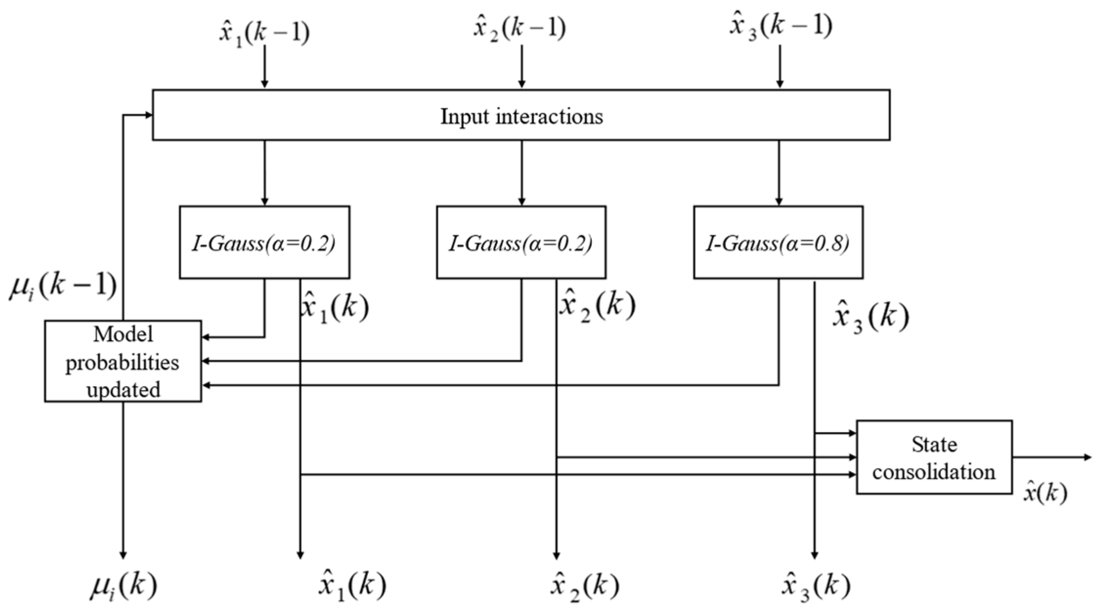
The fundamental idea of the interacting multiple model (IMM) is to match different motion models to the various motion patterns of maneuvering targets. To achieve the adaptive maneuvering frequency, three aforementioned improved models with different α are selected as three distinct models applied to the IMM algorithm. The switching of different α values is based on the maneuvering changes of the target. The specific process is illustrated in Figure 6. For detailed symbols and derivation formulae, please refer to [23].
To obtain accurate predictions of dynamic obstacle states for collision risk detection, a state-tracking system is established based on the I-Gauss model using the KF algorithm. The detailed process for establishing this system can be found in Appendix A.

3.2.2. SCD Model

To achieve an accurate obstacle avoidance for dynamic obstacles, it is essential to assess their potential collision risk based on their current motion states. This enables early avoidance measures. Therefore, an SCD model is proposed, as illustrated in Figure 7.
The blue dashed line represents the predicted trajectory of the dynamic obstacle, and the green dashed line represents the predicted trajectory of the AUV. Initially, the motion of the dynamic obstacle and the AUV are regarded as the I-Gauss model, and the motion state in the next step is predicted using the established KF prediction system. By varying the time step, the future trajectories of the AUV and the dynamic obstacles for the next N time steps can be obtained through Equation (16):
X k + 1 = Φ X k
where X k denotes the position at the current moment, X k + 1 represents the position at the next moment, and Φ is the state transition matrix of the motion model.
Subsequently, with the predicted position of the obstacles as the center, a dynamic obstacle collision risk zone is established, which is depicted as the shaded area in Figure 7. Its radius is calculated as Equation (17):
R k = t r Φ P k Φ T
where R k is the radius of the collision risk zone, P k represents the state covariance matrix of the prediction system based on Kalman filtering, and t r denotes the trace of the matrix.
Finally, if the predicted trajectory of the AUV falls into the obstacle’s collision risk zone between [ t k , t k + N ] , it is considered to have a collision risk. Establishing an outer circle around the corresponding collision risk zones in the current instance and the previous instance is denoted as the detection zone; the center of the detection zone is located as follows:
x = x k + | X k + 1 X k | + R k + 1 R k 2 c o s φ y = y t + | X k + 1 X k | + R k R k + 1 2 s i n φ φ = a r c t a n y k + 1 y k x k + 1 x k
Calculate the distance d from the center of the detection zone to the corresponding AUV trajectory. The formula for the improved repulsive force acting on the AUV is as Equation (19):
F r e p = k ( 1 d 1 R k ) 1 d 2
where k is the repulsion coefficient, and the method for its setting is introduced in Section 3.3. Unlike traditional methods, where the repulsion force points directly from the obstacle to the robot, in Equation (19), the direction of the repulsion force is perpendicular to the corresponding AUV trajectory’s radial direction.
The collision risk detection method of the SCD model is as shown in Algorithm 1.
Algorithm 1 The State-Tracking Collision Detection
Input: Observation position of moving obstacles, AUV position, and predicted number of steps N.
Step 1: Input the observed position of the moving obstacle at the previous moment and the actual position of the AUV, and the Kalman filter prediction system based on the improved Gaussian model (in Appendix A) is used to predict the dynamic obstacle and AUV position at the next N moments.
Step   2 :   Calculate   the   radius   of   the   obstacle   collision   risk   zone   R k at each moment according to Equation (17).
Step   3 :   If ,   at   any   time   of   the   prediction ,   | X ^ A U V X ^ O b s | R k , calculate the distance d from the center of the corresponding detection zone Equation (18) to the corresponding AUV trajectory.
Step 4: Calculate the repulsion using the improved Formula (19), and the direction is perpendicular to the radial direction of the corresponding AUV trajectory.

3.3. The SAPF

This has been a challenging issue in APF methods and their improvements in setting the coefficients for attraction and repulsion. If the repulsion coefficient is too large, it can lead to significant changes in the heading of the AUV, affecting its maneuverability. However, if the repulsion coefficient is too small, it may increase the risk of collisions. In environments with multiple dynamic obstacles, each with different motion states, it is necessary to adaptively adjust the repulsion coefficient based on real-time information about the target. The AUV’s velocity setting determines the step lengthening, thus influencing the voyage efficiency. It contributes to efficient obstacle avoidance by adjusting the step size.
The obstacle avoidance path should meet the requirements of being both safe and efficient. To achieve an AUV’s efficient and safe navigation, it is necessary to minimize its velocity and heading changes while maximizing its distance from dynamic obstacles. Therefore, the designed objective function is as Equation (20):
J = i = 1 M j = 1 N R i j l i j + ψ ψ 0 + V V 0
where M represents the number of obstacles in the field of view, N denotes the predicted number of steps, and R i j represents the collision risk radius of the i th obstacle at time j . The l i j is composed of three parts:
l i j = d + d 1 + d 2
where d , d 1 , d 2 represent the distance from the center of the detection area to the straight line of the AUV trajectory, and to the AUV’s current and predicted positions, as shown in Figure 8.
The objective function J takes the AUV heading angle, velocity, and distance to obstacles into consideration. When the objective function J reaches its minimum value, the planned obstacle avoidance route is the safest and most efficient. Therefore, the DOA problem is transformed into the optimization problem of minimizing the objective function, as described below:
M i n J s . t . ψ , V
To resolve the issue shown in Equation (22), the simulated annealing (SA) optimization algorithm is introduced; SA is a stochastic search algorithm used to solve large-scale combinatorial optimization problems. Its concept is inspired by the process of metal annealing and can be roughly described as follows: as the initial annealing temperature decreases, we continuously search for the optimal solution within feasible solutions. The SA algorithm has a probability of accepting solutions that are worse than the original solution. This ensures a convergence to the global optimum.
The SA algorithm is mainly composed of the Metropolis algorithm and annealing process, corresponding to the inner loop and outer loop, respectively [24]. The external circulation is the annealing process. When the solid is at a higher temperature, the solid is cooled according to a certain proportion according to the cooling coefficient. When the temperature drops to the termination temperature, the annealing process ends. The inner loop is the Metropolis algorithm. At each temperature of cooling, random disturbance produces several new solutions, calculates the corresponding objective function value of each new solution, and finds the optimal solution at this temperature. The optimization process for the objective function J using the SA algorithm is as shown in Algorithm 2.
Algorithm 2 The SA Algorithm Optimizes the Objective Function
Step 1: Set   initial   temperature   T 0 ,   end   temperature   T f ,   let   T = T 0 .   Generate   a   random   initial   solution   X 0 ,   and   compute   object   function   J ( X 0 ) .
Step 2: Set cooling coefficient λ ,   let   T = λ T , λ [ 0 , 1 ] .
Step   3   :   Add   stochastic   perturbation   to   the   current   solution X t   that   generates   a   new   solution   X t + 1   in   the   neighborhood ,   and   compute   the   corresponding   object   function   J ( X t + 1 ) ,   compute   Δ J = J ( X t + 1 ) J ( X t ) .
Step 4: If   Δ J < 0 ,   J X t + 1 is accepted; otherwise, the new one is decided according to the probability calculation.
Step 5: At temperature T , repeat steps 3 and step 4 for L times; L is a constant, and means the number of iterations of the inner loop.
Step 6: If   T = T f , end; else, return to step 2 to continue cooling.
The proposed dynamic obstacle avoidance strategy in the target-tracking process is illustrated in the flowchart depicted in Figure 9:

4. Simulation and Discussion

In this section, the following three questions are answered:
  • Q1. Can the SCD-SAPF algorithm solve the local minimum problem?
  • Q2. Is the proposed dynamic obstacle prediction based on the I-Gauss model effective?
  • Q3. The effectiveness and efficiency of the proposed SCD-SAPF algorithm for AUV dynamic obstacle avoidance must be validated. Can it adapt to a complex submarine environment?

4.1. Local Minimum Verification of the Proposed SCD-SAPF

To verify the feasibility of the SCD-SAPF algorithm, two scenarios were set up: one with a local minimum in a collinear situation and the other with non-collinearity. Simulation experiments were conducted for both scenarios using the traditional artificial potential field (T-APF) and the SCD-SAPF algorithms under the same conditions. The initial position of the AUV was set to (0, 0), with a step size of t = 0.5   s . Motion information for the tracked target and obstacles is provided in Table 3 and Table 4.
The parameters for T-APF were set as follows: obstacle influence radius ρ = 2 m , and attraction and repulsion coefficients k a t t = 1 and k r e p = 5 . In the SCD-SAPF algorithm, the prediction steps were uniformly set to 5. The simulation results for T-APF and SCD-SAPF are compared in Figure 10. The arrow points to the direction of motion of the AUV, moving obstacle and target.
As shown in Figure 10a,b, when sailing to the position near (1.3, 12.9), the repulsive forces generated by the two obstacles are equal in magnitude but opposite in direction to the target attraction force. The T-APF would drive the AUV into a deadlock, causing it to stop moving. However, with the strategy proposed in this paper, the repulsion coefficient is adjusted to ensure that the net force at this point is not zero. Under the action of the net force, the AUV safely avoids obstacles. As shown in Figure 10c,d, in the case of three collinear points, the improved repulsive force described in Equation (19) causes the AUV to move to the right, escaping the local minimum state and safely avoiding obstacles. The simulation results indicate that the proposed SCD-SAPF obstacle avoidance algorithm can solve the local minimum problem.

4.2. Dynamic Obstacle Prediction Verification

Based on the I-Gauss model proposed in Section 3.2.1 and the KF prediction system provided in the Appendix A, four different motion states were designed. Simulations were conducted for the CV, CA, adaptive Gauss model, and I-Gauss model to verify the performance of the system in predicting dynamic obstacles. The four motion states are presented in Table 5, Table 6, Table 7 and Table 8.
The simulation result is shown in Figure 11.
Using the root mean square error (RMSE) and mean error (ME) for the predicted positions, the performance of the model was compared. Figure 12 presents the prediction error results of the proposed state prediction system for obstacles with different motion states. It can be observed from Figure 12 that the proposed I-Gauss motion model has a higher accuracy than the existing CV, CA, and adaptive Gauss motion models. The RMSE in the x and y directions remains stable within the [0, 1] range, and the ME is stable within the range of [−0.1, 0.1]. This validates the effectiveness and stability of the established state prediction system based on the I-Gaussian model in predicting dynamic obstacles.

4.3. Feasibility and Effectiveness of the Proposed SCD-SAPF Algorithm

In the APF method, the robot moves toward the resultant force of attraction and repulsion. The coefficients of attraction and repulsion directly affect the resultant force acting on the robot, thereby influencing its direction of motion. However, setting these coefficients is a challenging task. If the repulsion coefficient is too large, it can lead to significant changes in the heading, potentially causing the tracked target to disappear from the field of view, resulting in target loss and not aligning with the actual motion of the AUV. In contrast, if the repulsion coefficient is too small, it may result in a poor obstacle avoidance performance. Moreover, for multi-objective OA, different targets have different motion states, making it impractical to use a uniform repulsion coefficient in the obstacle avoidance algorithm. It is necessary to dynamically adjust the repulsion coefficient based on real-time information about the targets. Therefore, this paper assumes a constant attraction coefficient of 1 and focuses on adjusting the repulsion coefficient to alter the robot’s motion direction. Specifically, repulsion coefficients of 1 and 10 were considered, and a comparison was made with the SCD-SAPF algorithm in the simulated experiments. The tracked targets and obstacle motion information are provided in Table 9.
The obstacle avoidance path with k r e p = 1 is shown in Figure 13a, and the path with k r e p = 10 was illustrated in Figure 13b. The path and the variation of the repulsion coefficient over time for the SCD-SAPF obstacle avoidance strategy are illustrated in Figure 13c,d. The maximum angular velocity and tracking time required for different repulsion coefficients are shown in Table 10. It can be observed that, with a small repulsion coefficient, the AUV can safely avoid Obstacle 1, but there is a collision risk with Obstacle 2. With a large repulsion coefficient, although the AUV can safely avoid Obstacle 2, the heading change during the avoidance of Obstacle 1 does not align with reality because of the high repulsion force. In the case of adaptive repulsion coefficients, different repulsion coefficients are applied based on the state information of different obstacles, allowing for the planning of reasonable paths to safely avoid all obstacles. The arrow points to the direction of motion of the AUV, moving obstacle and target.
The TAPF method provides the direction of motion for the AUV without changing the speed magnitude. With a constant step size, unreasonable paths may be planned in dynamic obstacle avoidance scenarios. To verify the superiority of the SCD-SAPF algorithm, we set up simulation scenario 4, and the motion information of the tracked target and obstacles is shown in Table 11.
As shown in Figure 14a, the obstacle is accelerating uniformly. When the AUV uses the TAPF method to avoid obstacles at a constant speed, in step 5, the obstacle is on the left side of the AUV, and, in step 6, the obstacle appears on the right side of the AUV. This results in two opposing forces along the X-axis, leading to the TAPF obstacle avoidance path shown in Figure 14a. Figure 13a also illustrates the obstacle avoidance path of the SCD-SAPF algorithm. Table 12 shows the tracking time, maximum acceleration, and maximum angular velocity required for the different algorithms. It can be observed that T-APF may plan ineffective paths with heading changes that violate AUV motion constraints. The proposed strategy, which includes velocity changes, avoids ineffective paths and effectively reduces significant changes in the heading. In this scenario, the tracking time is reduced by 14.7%, demonstrating an effective improvement in navigation efficiency. The arrow points to the direction of motion of the AUV, moving obstacle and target.
During underwater obstacle avoidance, due to the presence of complex environmental disturbances and sensor observation errors, AUV predictions of targets and obstacles may be subject to noise interference. In TAPF methods, the obstacle influence range is often a constant without considering the influence of noise. This oversight can sometimes lead to the failure of obstacle avoidance tasks. The tracked targets and obstacle motion information are provided in Table 13.
As shown in Figure 15b, with an obstacle avoidance radius of 2 m and no noise, the AUV can safely avoid the target. However, when Gaussian noise with a mean of 0 and a variance of 0.1 is introduced along the obstacle’s path, the AUV’s path intersects with the obstacle’s path. This occurs because there is an estimation error between the tracked value and the true value of the target, with the estimation value lagging behind the true value. The obstacle avoidance radius remains unchanged, resulting in the risk of collision. In contrast, the obstacle avoidance strategy proposed in this paper adjusts the obstacle avoidance radius based on the predicted error of the obstacle’s state. Figure 15a shows the obstacle avoidance path of the SCD-SAPF, and Figure 15c demonstrates the changes in the obstacle avoidance radius during the avoidance process. When noise is present, the obstacle avoidance radius increases, providing a safer execution of obstacle avoidance tasks by the AUV. Table 14 presents the obstacle avoidance results and tracking time for the different algorithms under various noise interferences. It can be observed that, even in the presence of noise interference, the obstacle avoidance strategy proposed in this paper can successfully navigate around obstacles with only a slight difference in obstacle avoidance time. The arrow points to the direction of motion of the AUV, moving obstacle and target.

5. Conclusions

Aiming at the problem of obstacle avoidance in dynamic environments, a dynamic obstacle avoidance strategy based on SCD-SAPF, which combines APF methods with target motion state tracking, is proposed. The SCD model construction of a motion state prediction system based on the dynamic obstacle model enables the assessment of collision risks between the AUV and obstacles. SAPF employs an SA algorithm to optimize the objective function for obtaining the optimal velocity and repulsion coefficients. This optimization allows for the calculation of the AUV’s obstacle avoidance path, addressing the inefficiencies and inadequacies of TAPF algorithms caused by fixed or poorly set parameters. The algorithm’s obstacle avoidance performance was investigated in various scenarios, and the following conclusions were drawn:
(1) The SCD-SAPF obstacle avoidance algorithm is proposed by considering the dynamic characteristics of obstacles and their associated risk zones. This enables the AUV to effectively accomplish dynamic obstacle avoidance tasks. The simulation results demonstrate that the algorithm can escape local minima and plan safe, reasonable, and efficient obstacle avoidance paths in various obstacle movement scenarios. This validates the effectiveness, feasibility, and robustness of the proposed algorithm.
(2) The I-Gauss motion model is proposed to address the mismatch issue between the true motion state of underwater moving targets and the tracking motion model. The simulation results indicate that this model further enhances the ability to adapt to different motion states compared with the adaptive Gauss model. When the target undergoes sudden maneuvers, it can quickly adapt to the new motion state. The Kalman filter-based state prediction system built on this model exhibits smaller errors, resulting in a better tracking performance of the target’s motion state.
(3) An SCD model is proposed that adaptively adjusts the obstacle range zone using the covariance information from the state prediction system. The simulation results demonstrate that the adjustable radius can effectively reduce the impact of noise, enhancing the robustness of the algorithm.
(4) The SAPF algorithm is proposed to optimize the avoidance path by designing an objective function that considers multiple future time steps and adjusting the repulsion coefficients and speed. The simulation results demonstrate that the stochastic nature of the SA algorithm addresses the issue of local minima by optimizing the repulsion coefficients and speed to ensure the efficiency of the avoidance path.
This paper focuses on the performance of the proposed SCD-SAPF algorithm, primarily addressing path design and optimization. The impact of the AUV and obstacle principal dimension on obstacle avoidance has not been discussed in detail, and related work will be conducted in future research.

Author Contributions

Conceptualization, Y.L., Y.M. and J.C.; methodology, Y.L. and J.C.; software, Y.M., C.Y. and X.M.; validation, Y.L., J.C. and C.Y.; formal analysis, Y.L.; investigation, Y.L. and J.C.; resources, Y.L. and J.C.; data curation, Y.M. and C.Y.; writing—original draft preparation, Y.L. and C.Y.; writing—review and editing, Y.L. and Y.M. visualization, Y.L. and X.M.; supervision, J.C.; project administration, Y.L. and J.C.; funding acquisition, Y.L. and J.C. All authors have read and agreed to the published version of the manuscript.

Funding

This work was financially supported by the National Natural Science Foundation of China (NO. 52071099, 52071104); Research Fund from National Key Laboratory of Autonomous Marine Vehicle Technology (NO. 2023-SXJQR-SYSJJ01).

Institutional Review Board Statement

Not applicable.

Informed Consent Statement

Not applicable.

Data Availability Statement

The data are contained within the article.

Acknowledgments

I would like to thank the National Key Laboratory of Autonomous Marine Vehicle Technology, Harbin Engineering University for providing a stimulating academic environment.

Conflicts of Interest

The authors declare no conflicts of interest.

Appendix A. The Dynamic Obstacle Prediction Model and System

All motion models in this paper are non-coupled co-ordinate models, assuming that the targets’ maneuvering processes in orthogonal directions are uncoupled.
(1)
CV model
The CV model is used to simulate the motion of the target when it undergoes uniform motion. In real scenarios, actual motion is subject to disturbances, and it is not always possible for the target to move uniformly in a straight line. When considering the random motion speed of the target due to the influence of random noise, we obtain
x ¨ t = ω t
where
E ω t = 0 E ω t ω t + τ = σ 2 δ τ
The state vector of the system is
x = x x ˙ T
The discrete state equation of the system can be expressed as follows:
x k + 1 = Φ C V x k + w C V k
where
Φ CV = e A CV T = 1 T 0 1
w C V k = 0 T e A C V T τ Γ C V ω k T + τ d τ = 0 T T τ 1 ω k T + τ d τ
The covariance of the discrete-time process noise is:
Q C V k = 0 T T τ 1 σ 2 T τ 1 d τ = 1 3 T 3 1 2 T 2 1 2 T 2 T σ 2
(2)
CA model
The CA model was employed to simulate the motion of the target undergoing uniform acceleration. It considers random variations in the target’s acceleration to be driven by stochastic noise. It is defined by the following equations:
x t = ω t
The state vector of the system is
x = x x ˙ x ¨ T
The discrete state equation of the system can be expressed as follows:
x k + 1 = Φ C V x k + w C V k
where
Φ C A = e A C A T = 1 T T 2 2 0 1 T 0 0 1
Q C V k = E w C A ( k ) w C A T ( k ) = T 5 20 T 4 8 T 3 6 T 4 8 T 3 3 T 2 2 T 3 6 T 2 2 T σ 2
(3)
Singer model
The Singer model is employed to describe the targets’ maneuvering acceleration using colored noise. It assumes that the time-correlation function of the target’s acceleration follows an exponential decay. Specifically, it is described by the following equations:
R a τ = E a t a t + τ = σ a 2 e α τ ,   a 0
where α is the target maneuvering frequency, σ a 2 is the variance of the acceleration noise, and α and σ a 2 are undetermined parameters that determine the targets’ maneuvering characteristics within ( t , τ ) .
KF tracking calculations require the driving noise to be Gaussian white noise. Therefore, Equation (A13) describing the zero-mean colored acceleration noise must undergo Wiener–Kolmogorov whitening to convert the colored noise into white noise. This process results in
a ˙ t = α a t + ω t
where the variance of the input ω t is
σ ω 2 = 2 α σ α 2
The variance of acceleration is:
σ α 2 = a max 2 3 ( 1 + 4 p max P 0 )
where a max is the maximum acceleration, p max is the probability when the acceleration is zero, and P 0 is the probability at the maximum acceleration.
The discrete state equation of the system can be expressed as follows:
x ( k + 1 ) = Φ ( k ) x ( k ) + w ( k )
where
Φ ( k ) = 1 T α T 1 + e α T α 2 0 1 1 e α T α 0 0 e α T
Q ( k ) = E w ( k ) w T ( k ) = q 11 q 21 q 31 q 12 q 22 q 32 q 13 q 23 q 33 × 2 α σ a 2
q 11 = ( 1 e 2 α T + 2 α T + 2 α 3 T 3 / 3 2 α 2 T 2 4 α T e α T ) / ( 2 α 5 ) q 12 = ( e 2 α T + 1 2 e α T + 2 α T e α T 2 α T + α 2 T 2 ) / ( 2 α 4 ) q 13 = ( 1 e 2 α T 2 α T e α T ) / ( 2 α 3 ) q 22 = ( 4 e α T 3 e 2 α T + 2 α T ) / ( 2 α 3 ) q 23 = ( e 2 α T + 1 2 e α T ) / ( 2 α 2 ) q 33 = ( 1 e 2 α T ) / ( 2 α 2 )
(4)
Kalman filter prediction system
The discrete-time state equation for the I-Gauss model can be expressed as:
x ( k + 1 ) = Φ ( k + 1 , k ) x ( k ) + U ( k ) a ¯ + w ( k )
where Φ ( k + 1 , k ) and Q ( k ) are the same as (A18) and (A19), and
U ( k ) = T + α T 2 / 2 + ( 1 + e α T ) / α ( T + α T 2 / 2 + ( 1 + e α T ) / α ) / α ( T ( 1 e α T ) / α ) α T ( 1 e α T ) / α ( 1 e α T ) α 1 e α T
a ¯ = a ¯ a ¯ ˙
w ( k ) = ( T + α T 2 / 2 + ( 1 e α T ) / α ) / α 2 ( 1 + α T + e α T ) / α 2 ( 1 e α T ) / α
The observation equation for the obstacle is described as:
z k = H k x k + v k
The KF prediction equation, as shown in Equations (A21) and (A25), is given by:
x ^ k | k = x ^ k | k 1 + K k z k H k x ^ k | k 1
x ^ k | k 1 = Φ k | k 1 x ^ k 1 | k 1 + U ( k 1 ) a ¯
K k = P k | k 1 H T k H k P k | k 1 H T k + R k 1
P k | k 1 = Φ k | k 1 P k 1 | k 1 Φ T k | k 1 + Q k 1
P k | k = I K k H k P ( k | k 1 )
where K k is the KF gain.
“Innovation” is a term used in KF to describe the difference between the observed measurement and the predicted state estimate, and can be expressed as:
r ( k ) = z ( k ) H ( k ) x ^ ( k | k 1 )
where r ( k ) is innovation and x ^ ( k | k 1 ) is an a priori or predicted system state.

References

  1. Li, J.; Li, C.; Chen, T.; Zhang, Y. Improved RRT Algorithm for AUV Target Search in Unknown 3D Environment. J. Mar. Sci. Eng. 2022, 10, 826. [Google Scholar] [CrossRef]
  2. Brcko, T.; Luin, B. A Decision Support System Using Fuzzy Logic for Collision Avoidance in Multi-Vessel Situations at Sea. J. Mar. Sci. Eng. 2023, 11, 1819. [Google Scholar] [CrossRef]
  3. Gao, W.; Han, M.; Wang, Z.; Deng, L.; Wang, H.; Ren, J. Research on Method of Collision Avoidance Planning for UUV Based on Deep Reinforcement Learning. J. Mar. Sci. Eng. 2023, 11, 2245. [Google Scholar] [CrossRef]
  4. Cheng, C.; Sha, Q.; He, B.; Li, G. Path Planning and Obstacle Avoidance for AUV: A Review. Ocean Eng. 2021, 235, 109355. [Google Scholar] [CrossRef]
  5. Li, D.; Wang, P.; Du, L. Path Planning Technologies for Autonomous Underwater Vehicles—A Review. IEEE Access 2019, 7, 9745–9768. [Google Scholar] [CrossRef]
  6. Panda, M.; Das, B.; Subudhi, B.; Pati, B.B. A Comprehensive Review of Path Planning Algorithms for Autonomous Underwater Vehicles. Int. J. Autom. Comput. 2020, 17, 321–352. [Google Scholar] [CrossRef]
  7. Taheri, E.; Ferdowsi, M.H.; Danesh, M. Closed-Loop Randomized Kinodynamic Path Planning for an Autonomous Underwater Vehicle. Appl. Ocean Res. 2019, 83, 48–64. [Google Scholar] [CrossRef]
  8. Yu, L.; Wei, Z.; Wang, Z.; Hu, Y.; Wang, H. Path Optimization of AUV Based on Smooth-RRT Algorithm. In Proceedings of the 2017 IEEE International Conference on Mechatronics and Automation (ICMA), Takamatsu, Japan, 6–9 August 2017; pp. 1498–1502. [Google Scholar]
  9. Wu, Q.; Chen, Z.; Wang, L.; Lin, H.; Jiang, Z.; Li, S.; Chen, D. Real-Time Dynamic Path Planning of Mobile Robots: A Novel Hybrid Heuristic Optimization Algorithm. Sensors 2020, 20, 188. [Google Scholar] [CrossRef] [PubMed]
  10. Khatib, O. Real-Time Obstacle Avoidance for Manipulators and Mobile Robots. In Proceedings of the 1985 IEEE International Conference on Robotics and Automation, St. Louis, MO, USA, 25–28 March 1985; Institute of Electrical and Electronics Engineers: Piscataway, NJ, USA, 2003; Volume 2, pp. 500–505. [Google Scholar]
  11. Fu, J.; Lv, T.; Li, B. Underwater Submarine Path Planning Based on Artificial Potential Field Ant Colony Algorithm and Velocity Obstacle Method. Sensors 2022, 22, 3652. [Google Scholar] [CrossRef] [PubMed]
  12. Li, D.; Pan, Z.; Deng, H.; Peng, T. 2D Underwater Obstacle Avoidance Control Algorithm Based on IB-LBM and APF Method for a Multi-Joint Snake-Like Robot. J. Intell. Robot. Syst. Theory Appl. 2020, 98, 771–790. [Google Scholar] [CrossRef]
  13. Zhang, W.; Wang, N.; Wu, W. A Hybrid Path Planning Algorithm Considering AUV Dynamic Constraints Based on Improved A* Algorithm and APF Algorithm. Ocean Eng. 2023, 285, 115333. [Google Scholar] [CrossRef]
  14. Hao, K.; Zhao, J.; Li, Z.; Liu, Y.; Zhao, L. Dynamic Path Planning of a Three-Dimensional Underwater AUV Based on an Adaptive Genetic Algorithm. Ocean Eng. 2022, 263, 112421. [Google Scholar] [CrossRef]
  15. Zhu, Z. Automatic Collision Avoidance Algorithm Based on Route-Plan-Guided Artificial Potential Field Method. Ocean Eng. 2023, 271, 113737. [Google Scholar] [CrossRef]
  16. Zhang, S.; Sang, H.; Sun, X.; Liu, F.; Zhou, Y.; Yu, P. A Real-Time Local Path Planning Algorithm for the Wave Glider Based on Time-Stamped Collision Detection and Improved Artificial Potential Field. Ocean Eng. 2023, 283, 115139. [Google Scholar] [CrossRef]
  17. Wang, D.; Wang, P.; Zhang, X.; Guo, X.; Shu, Y.; Tian, X. An Obstacle Avoidance Strategy for the Wave Glider Based on the Improved Artificial Potential Field and Collision Prediction Model. Ocean Eng. 2020, 206, 107356. [Google Scholar] [CrossRef]
  18. Fossen, T.I. Handbook of Marine Craft Hydrodynamics and Motion Control; John Wiley & Sons, Ltd.: Hoboken, NJ, USA, 2011. [Google Scholar]
  19. Rong Li, X.; Jilkov, V.P. Survey of Maneuvering Targettracking. Part I: Dynamic Models. IEEE Trans. Aerosp. Electron. Syst. 2003, 39, 1333–1364. [Google Scholar] [CrossRef]
  20. Singer, R. Estimating Optimal Tracking Filter Performance for Manned Maneuvering Targets. IEEE Trans. Aerosp. Electron. Syst. 1970, AES-6, 473–483. [Google Scholar] [CrossRef]
  21. Dang, J.; Huang, J. An Adaptive Gauss Model and Tracking Algorithm for Maneuvering Target. Telecommun. Eng. 2003, 43, 109–113+119. [Google Scholar]
  22. Gamse, S.; Nobakht-Ersi, F.; Sharifi, M. Statistical Process Control of a Kalman Filter Model. Sensors 2014, 14, 18053–18074. [Google Scholar] [CrossRef] [PubMed]
  23. Blom, H.A.P.; Bar-Shalom, Y. The Interacting Multiple Model Algorithm for Systems with Markovian Switching Coefficients. IEEE Trans. Autom. Control 1988, 33, 780–783. [Google Scholar] [CrossRef]
  24. Kirkpatrick, S.; Gelatt, C.D.J.; Vecchi, M.P. Optimization by Simulated Annealing. Science 1983, 220, 671–680. [Google Scholar] [CrossRef]
Figure 1. The overall framework of the DOA.
Jmse 12 00695 g001
Figure 2. The OA control of the AUV.
Jmse 12 00695 g002
Figure 3. AUV bow heading angular velocity constraints.
Jmse 12 00695 g003
Figure 4. The principle of the APF.
Jmse 12 00695 g004
Figure 5. Membership function.
Jmse 12 00695 g005
Figure 6. Adaptive flowcharts.
Jmse 12 00695 g006
Figure 7. The state-tracking collision detection model.
Jmse 12 00695 g007
Figure 8. The relative motion of AUV and dynamic obstacle.
Jmse 12 00695 g008
Figure 9. Flowchart of DOA strategy based on SCD-SAPF.
Jmse 12 00695 g009
Figure 10. The comparison between TAPF and SCD-SAPF.
Jmse 12 00695 g010
Figure 11. The error of dynamic obstacle prediction.
Jmse 12 00695 g011
Figure 12. RMSE and ME of the prediction error.
Jmse 12 00695 g012
Figure 13. The paths under different repulsion coefficients.
Jmse 12 00695 g013
Figure 14. Paths, velocity, and course under different algorithms.
Jmse 12 00695 g014
Figure 15. Paths in different algorithms.
Jmse 12 00695 g015
Table 1. The comparison of different OA methods based on the APF.
Control Plant2D/3D EnvironmentImprovementSimulation/ExperimentReference
Underwater Submarines3DReduce the number and length of inflection pointsSimulation[11]
Underwater Snake-like Robot2DVirtual target pointsSimulation[12]
AUV2DA* plus APF Simulation[13]
AUV3DCollision detection mechanismSimulation[14]
Smart Ship2DAssessing collision riskExperiment[15]
Wave Glider2DSolve local minimum, obstacle predictionSimulation[16]
Wave Glider2DSolve local minimum, collision predictionSimulation[17]
Table 2. Rules list of fuzzy adaptive coefficient.
λ r
VSSMBVB
a VSSMBVBVB
SSMBBM
MVSSMMM
BVSSMSS
VBVSSMSS
Table 3. Local minimal value scenario 1: non-collinear.
NumberInitial Position (m)Velocity (m/s)Acceleration (m/s2)
Target(0, 30)(0.5, 0.5)(0, 0)
Obstacle 1(−3.9, 10.6)(0.4, 0.3)(0, 0)
Obstacle 2(6.5, 21.8)(−0.3, −0.4)(0, 0)
Table 4. Local minimal value scenario 2: collinear.
NumberInitial Position (m)Velocity (m/s)Acceleration (m/s2)
Target(0, 30)(0, 0.6)(0, 0)
Obstacle(0, 20)(0, −0.4)(0, 0)
Table 5. Motion state 1.
Time (s)Initial Position (m)Velocity (m/s)Acceleration (m/s2)
XYXYXY
0~300002500
Table 6. Motion state 2.
Time (s)Initial Position (m)Velocity (m/s)Acceleration (m/s2)
XYXYXY
0~20000000.510
200~30010,00020,000100200−0.2−0.9
Table 7. Motion state 3.
Time (s)Initial Position (m)Velocity (m/s)Acceleration (m/s2)
XYXYXY
0~50000100.10
50~10012550051000
100~12037510005100−0.5
120~14047511005000.6
140~150575122051200
150~2006251340512−0.10
200~22075019400120.40
220~240830210081200
240~30011502420860−0.1
Table 8. Motion state 4.
Time (s)Initial Position (m)Velocity (m/s)Acceleration (m/s2)
XYXYXY
0~62 50 sin ( t 10 ) 50 cos ( t 10 ) 5 cos ( t 10 ) 5 sin ( t 10 ) 0 . 5 sin ( t 10 ) 0 . 5 cos ( t 10 )
Table 9. Scenario 3.
NumberInitial Position (m)Velocity (m/s)Acceleration (m/s2)
Target(0, 100)(0, 1)(0, 0)
Obstacle 1(−8.8, 20)(1, 0)(0, 0)
Obstacle 2(4.3, 126.5)(−0.1, −2)(0, 0)
Table 10. Courses and tracking time under different repulsion coefficients in scenario 3.
Repulsion CoefficientOA ResultsTracking Time (s)Maximum Angular Velocity (rad/s)
1Failure100.8410.394
10Success109.2641.553
SCD-SAPFSuccess101.1450.451
Table 11. Scenario 4.
NumberInitial Position (m)Velocity (m/s)Acceleration (m/s2)
Target(0, 20)(0, 0.5)(0, 0)
Obstacle(−10, 7.3)(0, 0)(0.5, 0)
Table 12. Courses and tracking time under different repulsion coefficients in scenario 4.
AlgorithmTracking Time (s)Maximum Acceleration (m/s2)Maximum Angular Velocity (rad/s)
TAPF50.15401.747
SCD-SAPF42.7560.4530.431
Table 13. Scenario 5.
NumberInitial Position (m)Velocity (m/s)Acceleration (m/s2)
Target(−1.5, 20)(0.5, 0)(0, 0)
Obstacle(10.8, 17.9)(−0.5, −0.3)(0, 0)
Table 14. OA results and tracking time under different noise.
AlgorithmOA ResultsTracking Time
NoiseNoiselessNoiseNoiseless
TAPFFailSuccess26.12625.183
SCD-SAPFSuccessSuccess26.11225.459
Disclaimer/Publisher’s Note: The statements, opinions and data contained in all publications are solely those of the individual author(s) and contributor(s) and not of MDPI and/or the editor(s). MDPI and/or the editor(s) disclaim responsibility for any injury to people or property resulting from any ideas, methods, instructions or products referred to in the content.

