
A Lightweight Model of Underwater Object Detection Based on YOLOv8n for an Edge Computing Platform

College of Intelligent Systems Science and Engineering, Harbin Engineering University, Harbin 150001, China
*
Author to whom correspondence should be addressed.
J. Mar. Sci. Eng. 2024, 12(5), 697; https://doi.org/10.3390/jmse12050697
Submission received: 23 March 2024
/
Revised: 18 April 2024
/
Accepted: 20 April 2024
/
Published: 23 April 2024
(This article belongs to the Special Issue Underwater Engineering and Image Processing)
Abstract
:The visual signal object detection technology of deep learning, as a high-precision perception technology, can be adopted in various image analysis applications, and it has important application prospects in the utilization and protection of marine biological resources. While the marine environment is generally far from cities where the rich computing power in cities cannot be utilized, deploying models on mobile edge devices is an efficient solution. However, because of computing resource limitations on edge devices, the workload of performing deep learning-based computationally intensive object detection on mobile edge devices is often insufficient in meeting high-precision and low-latency requirements. To address the problem of insufficient computing resources, this paper proposes a lightweight process based on a neural structure search and knowledge distillation using deep learning YOLOv8 as the baseline model. Firstly, the neural structure search algorithm was used to compress the YOLOv8 model and reduce its computational complexity. Secondly, a new knowledge distillation architecture was designed, which distills the detection head output layer and NECK feature layer to compensate for the accuracy loss caused by model reduction. When compared to YOLOv8n, the computational complexity of the lightweight model optimized in this study (in terms of floating point operations (FLOPs)) was 7.4 Gflops, which indicated a reduction of 1.3 Gflops. The multiply–accumulate operations (MACs) stood at 2.72 G, thereby illustrating a decrease of 32%; this saw an increase in the AP50, AP75, and mAP by 2.0%, 3.0%, and 1.9%, respectively. Finally, this paper designed an edge computing service architecture, and it deployed the model on the Jetson Xavier NX platform through TensorRT.
1. Introduction
Oceans contain abundant biological resources, and the utilization of these biological resources has strategic significance for economic development. Harnessing modern science and technology to enhance the rational upgrading of marine resource processing, as well as improving production efficiency, is a shared objective among numerous researchers. In recent years, owing to the proliferation of deep learning visual technology, object detection algorithms based on deep learning have superseded traditional approaches due to their exceptionally high accuracy [1]. In the past, underwater image data needed to be processed at a land center. However, processing large amounts of data on ground computing entities results in a high latency in the data transmission. In addition, communication conditions for such architectures are often not met in marine environments, and the information transmission rate of wireless communication systems at sea is relatively low—only short messages and low-speed message services can be transmitted. Although ocean satellite communication has a high speed, its cost is high, and the disadvantage of shore-based marine communication applications is that they cover a small coastal area [2]. To avoid the above two problems, an effective approach is to use a mobile edge computing platform to process the underwater data at the edge using edge nodes and edge servers.
As shown in Figure 1, mobile edge computing is a computing paradigm that uses mobile edge devices to provide relevant computing services at the network edge nodes instead of using the Elastic Compute Service (ECS) [3]. Edge computing nodes can be seen as the extension of the Internet of Things in the ocean. Edge computing has broad application prospects in water quality monitoring, pollution observation, marine resource exploration, etc. [4]. The advantage of an edge computing platform for underwater biological object detection is that it can achieve real-time processing and analysis, as well as reduce the cost of data transmission and storage. Additionally, edge computing platforms can process and analyze data in an underwater environment, thus avoiding the delay latency and instability of data transmission. In addition, for promotion of the accuracy and efficiency of detection, edge computing platforms can use machine learning algorithms to classify and identify underwater biological objects. This technology can be used for marine ecological environment monitoring, marine resource investigation, and marine scientific research, as well as in other fields.
Although edge platforms have natural advantages in performing marine organism detection tasks, due to hardware limitations, performing deep learning inference on mobile edge devices can easily lead to excessive load, thus resulting in an insufficient object detection capability so that the detection requirements cannot be met. In order to enable edge nodes to execute deep learning-based detection algorithms more efficiently, mature deep neural network models can be compressed to obtain lightweight models to better perform edge node computing tasks.
In this paper, the YOLOv8 [5] model was selected as the baseline model, and a new lightweight method based on neural network structure search and distillation is proposed to solve the problems of limited computing power, low recognition accuracy, high model complexity, and the high latency of edge nodes in an edge computing environment. Specifically, there are two steps: (1) Use the once for all neural architecture search algorithm and compress the YOLOv8 model backbone network to obtain a backbone network with low model complexity and high accuracy; (2) To compensate for the loss of accuracy, a mixed distillation method is designed, which integrates Channel-wise Distillation (CWD) [6] and KD [7] algorithms to achieve a synchronous distillation of the intermediate knowledge layers and to label knowledge in order to improve accuracy. Also, a service framework for the edge platform is designed to implement the model application of the edge computing platform.
2. Related Works
Currently, the primary lightweight methods for relevant models include neural architecture search, pruning, quantization, and knowledge distillation.
- Neural architecture search (NAS) is a method that involves an automated design of neural network structures. It mainly includes two key steps: search space design and search strategy selection. Search space design refers to defining the structural space of a neural network, such as the number of layers and convolutional kernels. The selection of a search strategy is to determine the search method and objective function, such as a genetic algorithm.
- Pruning is a technique used to reduce the number of parameters and computational complexity of neural networks. Pruning reduces the size and computational complexity of a model while maintaining its accuracy by removing unnecessary weights and connections from the neural network.
- Quantization is another method of optimizing neural networks. It mainly reduces the size and computational complexity of a model by reducing the accuracy of the model parameters and activation values, which usually leads to a certain degree of accuracy loss. Quantitative techniques can effectively reduce model storage space and computational requirements.
- Knowledge distillation is a model compression technique that utilizes large, high-performance teacher models to guide the training of small, compact student models. The core idea is to enable the student model to learn the output or intermediate representation of the teacher model so that the student model can approach the performance of the teacher model as closely as possible while maintaining a smaller model size.
The compression algorithm utilized in this article involves the neural structure search and knowledge extraction methods. The following are related research areas of these methods.
- (1)
- Neural architecture search
At present, the model of neural network structures is relatively complex and lacks theoretical guidance, which is not conducive for the use of deep learning. Therefore, researchers have begun to seek an automated way to independently design neural network structures, that is, through neural architecture search [8]. In the initial stage, Zoph et al. [9] sampled substructures (child networks) in the search space with a certain probability distribution through a controller by using reinforcement learning. Subsequently, the obtained structure is trained and its performance was tested on a validation set. Real et al. [10] first proposed a method similar to biological evolution, which mutates models with superior performance in randomly generated models and gradually eliminates network structures with poor performance to finally obtain the best performing model. However, such methods require a very large amount of computation, which greatly hinders research progress. Therefore, Pham et al. [11] proposed a parameter-sharing-based neural structure search, i.e., the efficientNet neural architecture via parameter sharing (ENAS) method. This method is a fast and low-cost automatic model design method. In ENAS, the controller searches for the best subgraph in a large computational graph while greatly reducing the computational overhead through a weight sharing among submodels, thus initiating the second stage of NAS. The above two stages have excessive overhead and are not suitable for practical model deployment. Researchers have begun to consider introducing relevant prior knowledge to reduce the cost of neural structure search algorithms, especially with limited computing resources available on mobile edge devices. Designing a resource-constrained mobile model is challenging. Based on the MobileNet search space, Stamoulis et al. [12] proposed the concept of a super kernel with a unified convolution kernel of 3 × 3 and 5 × 5. The two convolutions of five make the network a single-path structure. The practical deployment of deep learning models needs to adapt to different hardware platforms as the time spent on re-training is long. To address the practical deployment problem of the NAS model, Cai et al. [13] proposed a once for all (OFA) structure search algorithm to handle multiple deployment scenarios. This method separates the model training and structure search processes and trains an OFA network that supports multiple different structural settings such as depth, width, convolutional kernel size, and spatial resolution. Based on the actual deployment scenario, it simply selects the appropriate substructure in OFA without the need for an additional training process.
- (2)
- Knowledge distillation.
Knowledge distillation is like the teacher–student structure of human beings, providing knowledge through the pre-trained teacher models while the student models acquire teacher knowledge through distillation training. It can transfer complex teacher model knowledge to simple student models at a slight performance loss. Label knowledge is the potential information contained in a neural network’s final prediction output of sample data. Hinton et al. [7] first proposed knowledge distillation, which falls within this category. Due to the many uncertainties in the soft labels after adjusting the distillation temperature, Yang et al. [14] proposed using the label knowledge generated by the intermediate model updated by the teacher model in each training cycle to guide the student model. In order to fully explore the label information and remove interference, Muller et al. [15] used a subcategory distillation method to group the original labels and participate in soft label distillation learning. Owing to the output layer’s label knowledge’s incomplete information, some researchers hope to obtain more representative feature knowledge in the middle layer and transfer it to student models [16]. Differentiating between foreground and background regions in distillation is essential for object detection according to numerous techniques. By using L2 loss to force the feature maps within the student network RPN to resemble those of the teacher network, MIMIC [17] discovered that utilizing direct pixel level loss may negatively impact object detection performance. A proposal to extract fine-grained features near object anchor points was made by Wang et al. [18]. Zhang [19] achieved some outcomes by using the attention function to construct masks that distinguishes the foreground from the background. Recent research results [20] have also focused on the information found in every channel. Zhou and colleagues computed the mean activation value for every channel and matched the weighted discrepancies for every channel in the categorization. CSC [21] calculates the pairwise relationships between all spatial positions and all knowledge transfer channels. According to channel exchange [22], the data on each channel are universal and transferable between various models.
Object detection accuracy is significantly increased by using a deep learning-based approach. The two primary categories of CNN-based algorithms are two-stage object detection and single-stage object detection [23]. The detection problem is divided into two phases by the two-stage object detection technique. The algorithm in the first step creates candidate regions, which are then further refined and classified by the second stage algorithm. These algorithms include R-CNN [24], Fast R-CNN [25], Faster R-CNN [26], and Cascade R-CNN [27]. The one-stage object detection algorithm simultaneously detects and classifies objects, thus directly outputting the classification values of the objects’ location and probability coordinates. The common algorithm models range from examples such as the YOLO series [28,29,30,31,32], SSD [33], RetinaNet [34], FreeAnchor [35], FSAF [36], and FCOS [37]. Currently, there are also some lightweight studies on deep learning models. Fan [38] proposed a lightweight object detection algorithm, CM-YOLOv8, for coal mining working faces. They introduced an adaptive predefined anchor box tailored for the dataset and an L1-norm-based pruning method, which compresses the computational and parameter complexity of a model without affecting accuracy. Yang [39] proposed an automatic detection method based on an enhanced YOLOv8s model, which utilizes depthwise separable convolution (DSConv) to generate a substantial number of feature maps, thereby reducing computational complexity. Guo [40] proposed an underwater object detection method that optimized YOLOv8s by incorporating FasterNet as the backbone network. They modified the feature pyramid network to a fast feature pyramid network and introduced a lightweight C2f structure. The aforementioned methods have all introduced impressive solutions, with a particular emphasis on lightweight enhancements for YOLOv8s. However, deploying YOLOv8s on a Jetson Xavier NX proves challenging due to its size and complexity. Hence, this article adopted YOLOv8n as the baseline model.
3. Underwater Object Detection Based on Deep Learning
3.1. Underwater Image Enhancement Algorithm
Due to the complex underwater imaging environment, the quality of underwater images is usually low. The quality of the image has a significant impact on the results of object detection and recognition. High-quality images can easily lead to good features. Therefore, before conducting underwater object recognition, it is essential to first study underwater image and processing technology. As is well known, most underwater images suffer from blurring and color distortion problems. This is caused by the scattering and absorption of light, and particles in the water can also cause scattering phenomena during light propagation, thus resulting in a decrease in the contrast and blurring of the image, which is mainly caused by scattering phenomena.
This paper uses the Contrast Limited Adaptive Histogram Equalization (CLAHE) [41] algorithm to enhance underwater images. CLAHE is a image enhancement algorithm derived from Adaptive Histogram Equalization (AHE). The AHE algorithm changes the contrast of an image by calculating the local histogram of the image and redistributing brightness. This algorithm is more suitable for improving the local contrast of the image and obtaining more image details. Figure 2 shows the enhanced image result, which can be observed with the naked eye, where the processed image has a significant increase in contrast and brightness. Figure 3 shows a histogram that corresponds to the image in Figure 2. It can be seen from Figure 3 that the histogram of the CLAHE-processed image becomes smoother, thus making its texture details richer.
3.2. The Baseline Detection Model: YOLOv8
YOLOv8 is a SOTA (state-of-the-art) model based on the YOLO series that introduces new features and improvements to further increase adaptability and performance. It designs a new backbone network, uses a Anchor Free detection head to replace the previous Anchor base detection head, and designs a new loss function to train the new architecture. Figure 4 depicts the model’s precise structure.
- (1)
- The backbone network and NECK layer.
The largest modification to the NECK layer and YOLOv8 backbone network was the replacement of the C3 module with the C2f module. From Figure 5, it can be seen that C2f has more hop layer connections and additional split operations compared to C3. This approach enriches the gradient flow, which is conducive to feature fusion within the module and enhances feature information.
- (2)
- Anchor Free detection head.
The Anchor Free detection head was changed from the original coupling head to the current decoupling head. As shown in Figure 6, the position information and category information of the detection box awerere decoupled and extracted by two convolutional modules, respectively. Moreover, the Anchor base that has been used since YOLOv2 is abandoned here as the position information is directly obtained without relying on Anchors.
- (3)
- Loss function.
The loss function of YOLOv8 can be divided into the allocation strategy and loss calculation. Its allocation strategy refers to TOOD’s TaskAlignedAssignor, which uses the weighted results of regression and classification to choose positive samples. Its formula is shown in Equation (1):
where and are the hyperparameter constants. The prediction score for the annotated category is denoted by s, t is the IoU of the predicted box and the Ground Truth (GT) box, and the alignment degree can be measured by multiplying them. For each GT, for all predicted boxes and according to the GT category’s appropriate classification score, the weighted IoU of the predicted box and GT are used to obtain the alignment score metrics for association classification and regression. For each GT, the top K largest values are directly selected as positive samples based on the metric alignment score.
Classification loss and position regression loss are included in the loss computation; is still used for the classification loss even after confidence loss is subtracted, and the integral representation proposed in are bound by using and .
where y is a regression value for the label box, and are the integers closest to y. , ; , can be considered as the probability of the predicted point being compared to the left and right boundaries of the regression value. DFS is similar to performing cross entropy on the bounds of the expected value on the left and right, thus making it focus more quickly on the regression value.
The distance between the object box and the prediction box’s center is denoted by , where is the diagonal distance of the minimum bounding rectangle; and are the true length and width of the detection box, respectively; and w and h are the predicted detecting box’s dimensions.
4. Neural Architecture Search Algorithm
The once for all neural architecture search algorithm trains a one-time network that supports different architectures through separating the search from training to reduce costs. Without further training, it may rapidly pick from the network of OFA to obtain specific subnetworks.
4.1. OFA Large Model Training
The OFA network provides a large model that accommodates several subnetworks of various sizes by taking into account the four dimensions of crucial convolutional neural network (CNN) architecture, namely depth, width, kernel size, and resolution. The fine tuning of the depth and convolutional kernel processes are shown in Figure 7 and Figure 8, respectively, where the OFA network divides the CNN model into a series of units with progressively smaller feature map sizes and an increasing number of channels. Each unit is composed of a series of layers, and if the feature map size decreases, only the first layer has a step size of 2. All the other layers in the unit have a step size of 1. The OFA large network includes several subnetworks of various sizes, including tiny subnetworks nestled inside larger subnetworks. To prevent interference between subnetworks, the OFA network gradually executes the training sequence from large subnetworks to small subnetworks. Then, the OFA network starts by using the greatest possible kernel size, depth, and width to train the neural network. Smaller subnets are gradually added to the sampling space to gradually fine tune the network to support smaller subnets. In particular, it offers elastic kernel size, which may be chosen at each layer from 3, 5, 7 after training the largest network, and the depth and width stay at their maximum values. Following that, the elastic width is supported and then the depth in turn. Throughout the training process, the resolution is elastic, which is achieved by varying the size of the picture samples for every training data batch.
4.2. Dedicated Model Deployment for OFA
After training the OFA network, then obtaining specific subnetworks for the specified deploying situation is the next step. The goal is to search for neural networks that meet the efficiency constraints of the target hardware (such as latency and energy) while maximizing precision. We do not currently require any sort of training expenditures since the OFA network separates the process of training the models from the search for neural architectures. In addition, in order to provide quick feedback on the quality of a model, OFA has developed neural network twins that can forecast the delay and accuracy of a particular neural network architecture. By substituting the anticipated accuracy/delay for measurement accuracy/waiting time, it eliminates the expense of redundant searches.
4.3. Application of the OFA Network in Object Detection
The OFA network demonstrates outstanding performance in classification tasks, and this paper extends its application to detection tasks. This paper uses the OFA neural network search algorithm to optimize the backbone network of the object detection algorithm. This paper dose not retrain the OFA large model, it only uses the dedicated model search algorithm of the OFA network. The search is constrained by the model’s computational complexity (in terms of FLOPs) and accuracy, where the large OFA model is already trained on the ImageNet dataset. With consideration of the target hardware and latency limitations, an evolutionary search is performed based on neural network twins to obtain specialized subnetworks. As the cost of using neural network twins for search can be negligible, this paper does not spend too much time obtaining subnetworks. After obtaining the subnetworks, the subnetworks are then transplanted into existing object detection algorithms, and the NECK layer of the object detection algorithm is fine tuned. A new object detection model is retrained to test its effectiveness. The process is shown as Figure 9.
The OFA sub network used in this paper is based on MobileNetV3, with a width multiplier of 1.2 (this supports an elastic depth of (2, 3, 4), an elastic scaling ratio of (3, 4, 6), and an elastic kernel size of (3, 5, 7) for each stage). This paper uses a subset of ImageNet for testing, which includes 2000 images (~250 M). Then, for constructing the accuracy prediction and complexity prediction functions, the searching is started with a neural architecture that is constrained by FLOPs. The search algorithm employed is an evolutionary algorithm. In each generation, the population size is set to 10, and the total number of generations to be searched is 500. The probability of mutation in the evolutionary search is 0.1, with a mutation ratio of 0.5 for the networks generated in each generation through mutation. Evolutionary algorithms explore the structural space, and their adaptability is gauged by accuracy and complexity functions. Upon reaching the specified number of iterations, the optimal subnet information and weights are preserved.
The backbone network resulting from the NAS search fulfills the anticipated requirements of this paper in terms of FLOPs. However, the network derived from the search process differs from the original YOLOv8n network, thereby exhibiting inadequate adaptability. A direct migration to this network may lead to a reduction in detection accuracy. Consequently, this paper opted to employ the knowledge distillation algorithm to enhance accuracy.
5. Knowledge Distillation Algorithm
In this paper, a neural network distillation architecture that objectifies both the label knowledge and the intermediate knowledge layer simultaneously was designed by utilizing the detection ability of the large model as a prior basis. When changing the object detection model of the backbone network for training, the intermediate layer features of the large model are added, and the output layer features correct the intermediate and output layers of the small model to obtain a more accurate model.
5.1. Basic Principles of Knowledge Distillation
A model can be seen as a “black box” by knowledge distillation because knowledge is a relationship that maps from inputs to outputs. Its basic process is shown in Figure 8. Therefore, a teacher network can be trained first; afterward, the student network’s aim, Q, can serve as the output result of the teacher network in order to instruct the student network so that P, the student network’s result, approaches Q. Therefore, its loss function can be designated as
where y is the single-hot transformation of the real label, q is the teacher network’s output result, p is the student network’s output result, and is the cross entropy. The loss function here is to add the cross entropy with the teacher network output as the label on the basis of the original cross entropy.
The class probability is generated by using the output layer of transformation . Then, is compared with the other logistic regressions and the probability for each class is calculated. The formula is as follows:
This formula, called softmax, yields the probability of every class based on a logit if T is around 0. It is identical to one-hot encoding, where other values will be nearer to 0 and the maximum value will be nearer to 1 if T is near to 0. The overall distribution of the final outcomes will be smoother if T is greater, where it acts as a smoothing function to retain similar information. Formula (5) states that if T equals infinity, it approximates a uniform distribution.
5.2. Channel-Wise Distillation
Channel-wise distillation (CWD) is a knowledge distillation method for knowledge across channels. In order to better utilize the knowledge in each channel, the CWD algorithm proposes to gently adjust the activation function of the corresponding channel between the networks of teachers and students. In Figure 10, the fundamental procedure is displayed. To achieve this, CWD was used to first convert the activation of the channel into a probability distribution, which can be measured using probability distance measures (such as KL divergence). Figure 11 illustrates how the activation of several channels tends to encode the scene category’s salience in the input image. CWD, as a revolutionary channel refinement paradigm, can let student networks learn from teacher networks with higher model capabilities.
Let T and S denote the teacher and student networks, and let and denote the activation mappings from T and S, respectively. The following is the channel distillation loss:
In the CWD algorithm, the activation values are transformed into probability distributions using , as shown below:
where i indicates the channel’s spatial location, indicates the channel, and T is a hyperparameter (temperature). The probability softens with increasing T, thus indicating the need to concentrate on a greater geographical region for each channel. By applying softmax normalization, the influence of the magnitude between large and compact networks is eliminated. This normalization is helpful for KD. If the number of channels between teachers and students does not match, the student network’s channel count is upsampled using the convolutional layer. Then, evaluates the differences in the channel distribution of teacher networks and student networks by using KL divergence as follows:
KL divergence is a kind of asymmetric metric. It is evident from the above equation that in order to reduce KL divergence, should be as large as if is large. Additionally, KL divergence is only somewhat minimized if is small. Therefore, student networks tend to focus on foreground salience by generating a similar activation distribution. The activation associated with the teacher network’s background area has a relatively small impact on learning.
5.3. The Distillation Structure Design of This Paper
To achieve a comprehensive understanding of teacher characteristics, this paper integrates the channel-wise distillation and knowledge distillation algorithms to devise a novel knowledge distillation architecture, as depicted in Figure 12. Initially, the paper utilizes CWD to extract the feature pyramid network (FPN) by distilling the regions with the most abundant feature information. This enables the feature layer of the student network to assimilate prior learning outcomes, thereby enhancing the salience of the feature pyramid generated by the student network. Moreover, KL divergence is incorporated into the HEAD section to expedite the convergence of the student network and to offer guidance during the training process. Weighting the loss of the HEAD segment of YOLOv8n serves to stabilize the outcomes.
CWD is used at the NECK module to distill the feature pyramid, and KL divergence is used at the beginning of the output head to achieve soft label distillation. Finally, the two are added with a certain weight to obtain the total distillation loss and to participate in backpropagation together with the conventional loss.
6. Experimental Analysis
6.1. Dataset and Experimental Environment Settings
The 2020 China Underwater Vehicle (Zhanjiang) Competition officially donated the underwater biological picture dataset used in this paper. There are 5534 photos of starfish, scallops, sea cucumbers, and sea urchins in the collection. Some low-quality photographs were chosen for augmentation since many of the images in the original dataset had low contrast and color distortion. The dataset was improved using the CLAHE underwater image enhancement technique. The dataset for this paper consists of 7930 photos altogether, which are created by combining the enhanced and original photographs.
The experimental platform processor is E5-2660v4 CPU, the GPU is GTX2080, and the computing environment is PyTorch 1.1.4.
6.2. Baseline Model Detection Experiment
This paper first conducted pre-experiments on underwater biological objects, selecting several typical models for experimental comparison to demonstrate the superiority of choosing YOLOv8n. To select the lightweight versions of various models, the ResNet minimum network ResNet18 was selected as the backbone network for non YOLO series models, while, for the YOLO series models, the minimum network for each version (v3 and v4 are not proposed as lightweight models) was selected.
From Table 1, it can be seen that the classic two-stage and one-stage object detection algorithms, even if their backbone network is replaced with the smallest version of ResNet (i.e., ResNet18), still have a much higher computational complexity FLOPs than the lightweight version models proposed by the YOLO series. In the lightweight version models of the YOLO series, YOLOv8n has a computational complexity and model size second only to YOLOv5n, but its detection accuracy (mAP) is much higher than YOLOv5n. Therefore, this paper chose YOLOv8n as the baseline model for the experiment.
6.3. Experimental Results after Compression Optimization
This paper first used pre-trained large-scale models in an OFA network to conduct a structural search in the experimental environment of this paper. The model accuracy (mAP) and model complexity (FLOPs) metrics were used as search objectives for 300 iterations to obtain the model parameters and model structure files. The OFA algorithm uses MolileNetv3 as its basic large model, and, after 500 iterations, its accuracy mAP value and model complexity (FLOPs) were 72.3% and 2.4 GFlops, respectively.
The YOLOv8n’s backbone network was swapped out for one that the OFA method repeatedly searches for in training; then, the model results are obtained. To increase the model’s accuracy and enhance the training procedure, the training procedure incorporates the distillation architecture suggested in this research. The teacher network used in this paper is the YOLOv8s model.
From Table 2 and Table 3, as well as Figure 13, it can be concluded that the performance of the YOLOv8n network model has made much progress compared to before adopting the OFA algorithm and the distillation algorithm. In terms of model complexity, the compressed model exhibited a computational complexity of 7.4 Gflops and a MAC value of 2.7 G, which aligns closely with the smallest YOLOv5n model within the YOLO series. In comparison to its performance prior to compression, there has been a reduction in complexity by 1.3 Gflops and a decrease in the MAC value by approximately 32%. Due to the compensatory effect of the distillation algorithm, the compressed YOLOv8 also achieved the best precision of the YOLO series small models. From Figure 13, it can be seen that the confidence level of each object increased by nearly 10 points. In actual deployment, the confidence threshold can be increased to filter similar objects and improve generalization. Compared with YOLOv8n, the compressed YOLOv8 increased AP50, AP75, and mAP by 2.0%, 3.0%, and 1.9%, respectively. From the comprehensive calculation complexity and model precision, in summary, the YOLOv8n model, which was compressed for this paper, is currently the better tiny model in the YOLO family, and it is also the most suitable network for being deployed on an edge computing platform.
7. Edge Computing Platform Applications
This chapter mainly studies the deployment and application of the edge computing platform of the object detection algorithm that was constructed with Jetson Xavier NX (which is shown in Figure 14) as the deployment platform used to improve YOLOv8n. This chapter also shows how the model was accelerated through TensorRT, which further improves the detection speed of the model, as well as how the server framework was used to implement the streaming of video and the post-processing of detection data.
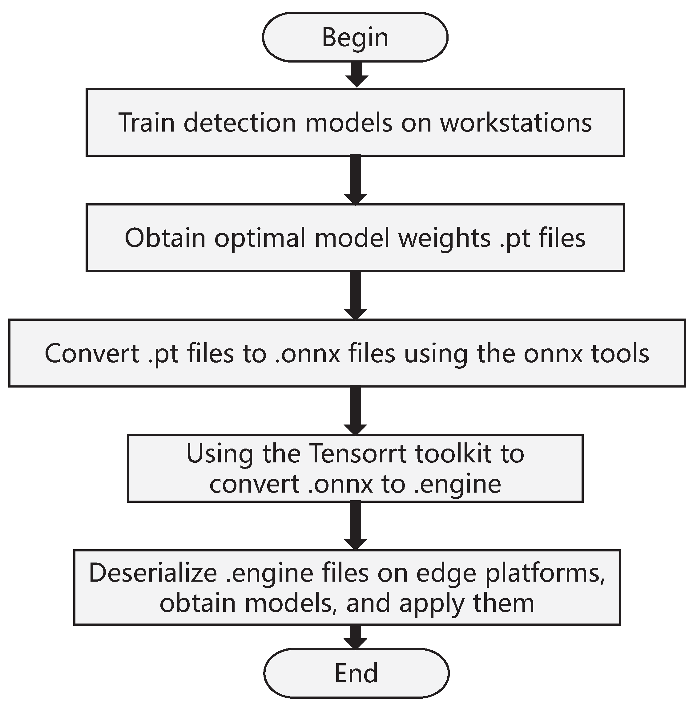
TensorRT is a software development suite proposed by NVIDIA (Santa Clara, CA, USA) for optimizing trained deep learning models to achieve high-performance inference. TensorRT includes a deep learning inference optimizer for trained deep learning models, as well as a runtime engine for execution, which can run deep learning models with a higher throughput and lower latency. In this paper, the model file is first converted into an onnx intermediate format file, and the middleware is converted into an engine file using the compiler in the TensorRT suite. Afterward, the C++/Python API interface in the middleware can be called to implement end-to-end model applications. The specific process is shown in Figure 15.
This paper uses an edge computing platform as an edge computing server that can complete data collection and calculation in a production environment. In the framework of network programming, the model compiled by TensorRT is used to provide application services. This paper implements the video stream push based on TensorRT and Django frameworks. Django is a Python-based network service framework (which can easily provide the required network services). The main process of the video streaming is as follows:
- Using the OpenCV and V4L2 frameworks to capture images from USB-driven cameras;
- Processing image information using the detection model compiled by TensorRT, which is then pushed to the FFmpeg process;
- Using FFmpeg to implement the RTMP protocol (RTMP video stream is a real-time video stream protocol) to push the video streams, with the proxy server being the Nginx server.
Through the Nginx service, video stream access can be achieved on a local area network or external network. The V4L2 framework is a video source capture driver framework that is used in Linux systems. It is widely used in embedded devices, mobiles, and personal computer devices for video capture. FFmpeg is a set that can be used for recording, and it is an open-source computer program that converts digital audio and video into streams. Nginx is a high-performance HTTP and reverse proxy server, and it is characterized by low memory consumption and strong concurrency, and it is suitable for network IO processing on edge computing platforms. The control of video streams is determined by the requests sent by the client to the Django framework.
From Figure 16, it can be seen that the application architecture of this paper is divided into four layers and the program processing order is bottom-up. The first layer is the basic tool for edge nodes, which is the V4L2 driver program for collecting image information; the TensorRT model is used for image processing; the UNIX network IO is used for communication, with the second layer serving as the FFmpeg tool for recommending video streams; the Django framework is used for providing network services; the SQLite database is used to store the data; the third layer merely utilizes Nginx’s ability to handle high concurrency to improve concurrency by a few points; and the fourth layer is the application services that can play FLV videos through web pages or can directly call RTMP video streams through other decoding tools.
Figure 17 illustrates the remote access application of the edge computing platform. The edge computing platforms can be deployed as edge servers in offshore shallow waters. Through the deployment of an optical fiber communication network underwater, a water–shore network covering both underwater and shore areas can be established. This setup facilitates information sharing and collaborative work between underwater devices and shore-based servers. The edge servers have the capability to process and analyze underwater data in real-time. They can detect and statistically analyze marine organisms near the shore, thus enabling quick responses to the requirements of onshore clients. This integration is suitable for intelligent marine ranching, intelligent marine ecological protection, and other scenarios.
8. Conclusions
Edge platforms have natural advantages in performing marine organism detection tasks. However, due to hardware limitations, performing deep learning inference on mobile edge devices can easily lead to excessive load, thus resulting in insufficient object detection capabilities and an inability to meet task detection requirements. To enable edge nodes to execute deep learning algorithms more efficiently, this paper proposes a compression process that reduces model computational complexity and improves accuracy. (The technique proposed in this paper can better perform edge detection tasks.) Multiple deep learning-based object detection baseline models were tested in this paper. YOLOv8n, based on detection accuracy and computational complexity, was chosen as the target model for the compression method. Then, the OFA algorithm was used for structural searching to obtain the optimal lightweight backbone network. Simultaneously, CWD and KD distillation were combined during the training phase, thus making use of the teacher network’s past knowledge to increase model accuracy. The compressed YOLOv8n in this paper surpasses the performance of the minimal lightweight models in the YOLO family in terms of accuracy and overall computing complexity with good application prospects.
Author Contributions
Conceptualization, P.L. and Y.F.; methodology, P.L., Y.F. and L.Z.; software, Y.F. and L.Z.; writing—original draft preparation, P.L. and Y.F.; writing—review and editing, L.Z. and Y.F.; funding acquisition, L.Z. and P.L. All authors have read and agreed to the published version of the manuscript.
Funding
Supported by State Key Laboratory of Robotics and Systems (HIT)(SKLRS-2023-KF-17).
Institutional Review Board Statement
Not applicable.
Informed Consent Statement
Not applicable.
Data Availability Statement
The original contributions presented in the study are included in the article.
Conflicts of Interest
The authors declare no conflicts of interest.
References
- Zou, Z.; Chen, K.; Shi, Z.; Guo, Y.; Ye, J. Object Detection in 20 Years: A Survey. Proc. IEEE 2023, 111, 257–276. [Google Scholar] [CrossRef]
- Wang, T.; Zhang, G.; Bhuiyan, M.Z.A. A novel trust mechanism based on fog computing in sensor–cloud system. Future Gener. Comput. Syst. 2020, 109, 573–582. [Google Scholar] [CrossRef]
- Qiu, T.; Zhao, Z.; Zhang, T. Underwater Internet of Things in smart ocean: System architecture and open issues. IEEE Trans. Ind. Inform. 2019, 16, 4297–4307. [Google Scholar] [CrossRef]
- Mary, D.R.K.; Ko, E.; Kim, S.G. A systematic review on recent trends, challenges, privacy and security issues of underwater internet of things. Sensors 2021, 21, 8262. [Google Scholar] [CrossRef] [PubMed]
- Hussain, M. YOLO-v1 to YOLO-v8, the rise of YOLO and its complementary nature toward digital manufacturing and industrial defect detection. Machines 2023, 11, 677. [Google Scholar] [CrossRef]
- Shu, C.; Liu, Y.; Gao, J.; Yan, Z.; Shen, C. Channel-wise knowledge distillation for dense prediction. In Proceedings of the IEEE/CVF International Conference on Computer Vision, Montreal, BC, Canada, 11–17 October 2021; pp. 5311–5320. [Google Scholar]
- Hinton, G.; Vinyals, O.; Dean, J. Distilling the knowledge in a neural network. arXiv 2015, arXiv:1503.02531. [Google Scholar]
- Li, H.Y.; Wang, N.N.; Zhu, M.R.; Yang, X.; Gao, X.B. Recent Advances in Neural Architecture Search: A Survey. Ruan Jian Xue Bao J. Softw. 2022, 33, 129–149. [Google Scholar]
- Zoph, B.; Le, Q.V. Neural architecture search with reinforcement learning. arXiv 2016, arXiv:1611.01578. [Google Scholar]
- Zoph, B.; Vasudevan, V.; Shlens, J.; Le, Q.V. Learning Transferable Architectures for Scalable Image Recognition. In Proceedings of the IEEE/CVF Conference on Computer Vision and Pattern Recognitio, Salt Lake City, UT, USA, 18–23 June 2018; pp. 8697–8710. [Google Scholar]
- Pham, H.; Guan, M.; Zoph, B. Efficient neural architecture search via parameters sharing. In Proceedings of the International Conference on Machine Learning, PMLR, Stockholm, Sweden, 10–15 July 2018; pp. 4095–4104. [Google Scholar]
- Stamoulis, D.; Ding, R.; Wang, D. Single-path nas: Designing hardware-efficient convnets in less than 4 hours. In Proceedings of the Machine Learning and Knowledge Discovery in Databases: European Conference—ECML PKDD 2019, Würzburg, Germany, 16–20 September 2019; Proceedings, Part II. Springer International Publishing: Cham, Switzerland, 2020; pp. 481–497. [Google Scholar]
- Cai, H.; Gan, C.; Wang, T. Once-for-all: Train one network and specialize it for efficient deployment. arXiv 2019, arXiv:1908.09791. [Google Scholar]
- Yang, C.; Xie, L.; Su, C. Snapshot distillation: Teacher-student optimization in one generation. In Proceedings of the IEEE/CVF Conference on Computer Vision and Pattern Recognition, Long Beach, CA, USA, 15–20 June 2019; pp. 2859–2868. [Google Scholar]
- Müller, R.; Kornblith, S.; Hinton, G. Subclass distillation. arXiv 2020, arXiv:2002.03936. [Google Scholar]
- Romero, A.; Ballas, N.; Kahou, S.E.; Chassang, A.; Gatta, C.; Bengio, Y. Fitnets: Hints for thin deep nets. arXiv 2014, arXiv:1412.6550. [Google Scholar]
- Li, Q.; Jin, S.; Yan, J. Mimicking very efficient network for object detection. In Proceedings of the IEEE Conference on Computer Vision and Pattern Recognition, Honolulu, HI, USA, 21–26 July 2017; pp. 6356–6364. [Google Scholar]
- Wang, T.; Yuan, L.; Zhang, X.; Feng, J. Distilling object detectors with fine-grained feature imitation. In Proceedings of the IEEE/CVF Conference on Computer Vision and Pattern Recognition, Long Beach, CA, USA, 15–20 June 2019; pp. 4933–4942. [Google Scholar]
- Zhang, L.; Ma, K. Improve object detection with feature-based knowledge distillation: Towards accurate and efficient detectors. In Proceedings of the International Conference on Learning Representations, Virtual, 3–7 May 2021. [Google Scholar]
- Zhou, Z.; Zhuge, C.; Guan, X.; Liu, W. Channel distillation: Channel-wise attention for knowledge distillation. arXiv 2020, arXiv:2006.01683. [Google Scholar]
- Park, S.; Heo, Y.S. Knowledge distillation for semantic segmentation using channel and spatial correlations and adaptive cross entropy. Sensors 2020, 20, 4616. [Google Scholar] [CrossRef] [PubMed]
- Shi, Y.; Deng, A.; Deng, M. Transferable adaptive channel attention module for unsupervised cross-domain fault diagnosis. Reliability Engineering and System Safety 2022, 226, 108684. [Google Scholar] [CrossRef]
- Cheng, R. A survey: Comparison between Convolutional Neural Network and YOLO in image identification. J. Phys. Conf. Ser. 2020, 1453, 012139. [Google Scholar] [CrossRef]
- Pedersen, M.; Haurum, J.B.; Gade, R.; Moeslund, T.B. Detection of marine animals in a new underwater dataset with varying visibility. In Proceedings of the IEEE/CVF Conference on Computer Vision and Pattern Recognition Workshops, Long Beach, CA, USA, 15–20 June 2019; pp. 18–26. [Google Scholar]
- Ren, S.; He, K.; Girshick, R.; Sun, J. Faster R-CNN: Towards real-time object detection with region proposal networks. IEEE Trans. Pattern Anal. Mach. Intell. 2016, 39, 1137–1149. [Google Scholar] [CrossRef] [PubMed]
- Siddiqui, S.A.; Salman, A.; Malik, M.I.; Shafait, F.; Mian, A.; Shortis, M.R.; Harvey, E.S. Automatic fish species classification in underwater videos: Exploiting pre-trained deep neural network models to compensate for limited labelled data. ICES J. Mar. Sci. 2018, 75, 374–389. [Google Scholar] [CrossRef]
- Cai, Z.; Vasconcelos, N. Cascade R-CNN: High Quality Object Detection and Instance Segmentation. IEEE Trans. Pattern Anal. Mach. Intell. 2021, 43, 1483–1498. [Google Scholar] [CrossRef]
- Redmon, J.; Divvala, S.; Girshick, R.; Farhadi, A. You only look once: Unified, real-time object detection. In Proceedings of the IEEE Conference on Computer Vision and Pattern Recognition, Las Vegas, NV, USA, 27–30 June 2016; pp. 779–788. [Google Scholar]
- Redmon, J.; Farhadi, A. YOLO9000: Better, faster, stronger. In Proceedings of the IEEE Conference on Computer Vision and Pattern Recognition, Honolulu, HI, USA, 21–26 July 2017; pp. 7263–7271. [Google Scholar]
- Farhadi, A.; Redmon, J. Yolov3: An incremental improvement. arXiv 2018, arXiv:1804.02767. [Google Scholar]
- Diwan, T.; Anirudh, G.; Tembhurne, J.V. Object detection using YOLO: Challenges, architectural successors, datasets and applications. Multimed. Tools Appl. 2022, 82, 9243–9275. [Google Scholar] [CrossRef]
- Li, P.; Fan, Y.; Cai, Z.; Lyu, Z.; Ren, W. Detection Method of Marine Biological Objects Based on Image Enhancement and Improved YOLOv5S. J. Mar. Sci. Eng. 2022, 10, 1503. [Google Scholar] [CrossRef]
- Liu, W.; Anguelov, D.; Erhan, D.; Szegedy, C.; Reed, S.; Fu, C.Y.; Berg, A.C. SSD: Single shot multibox detector. In Proceedings of the European Conference on Computer Vision, Amsterdam, The Netherlands, 11–14 October 2016; pp. 21–37. [Google Scholar]
- Lin, T.Y.; Goyal, P.; Girshick, R.; He, K.; Dollár, P. Focal loss for dense object detection. In Proceedings of the IEEE International Conference on Computer Vision, Venice, Italy, 22–29 October 2017; pp. 2980–2988. [Google Scholar]
- Zhang, X.; Wan, F.; Liu, C.; Ji, R.; Ye, Q. Freeanchor: Learning to match anchors for visual object detection. In Proceedings of the 33rd Conference on Neural Information Processing Systems (NeurIPS 2019), Vancouver, BC, Canada, 8–14 December 2019; Volume 32. [Google Scholar]
- Zhu, C.; He, Y.; Savvides, M. Feature selective anchor-free module for single-shot object detection. In Proceedings of the IEEE/CVF Conference on Computer Vision and Pattern Recognition, Long Beach, CA, USA, 15–20 June 2019; pp. 840–849. [Google Scholar]
- Tian, Z.; Shen, C.; Chen, H.; He, T. Fcos: Fully convolutional one-stage object detection. In Proceedings of the IEEE/CVF International Conference on Computer Vision, Seoul, Republic of Korea, 27 October–2 November 2019; pp. 9627–9636. [Google Scholar]
- Fan, Y.; Mao, S.; Li, M.; Wu, Z.; Kang, J. CM-YOLOv8: Lightweight YOLO for Coal Mine Fully Mechanized Mining Face. Sensors 2024, 24, 1866. [Google Scholar] [CrossRef] [PubMed]
- Yang, G.; Wang, J.; Nie, Z.; Yang, H.; Yu, S. A Lightweight YOLOv8 Tomato Detection Algorithm Combining Feature Enhancement and Attention. Agronomy 2023, 13, 1824. [Google Scholar] [CrossRef]
- Guo, A.; Sun, K.; Zhang, Z. A lightweight YOLOv8 integrating FasterNet for real-time underwater object detection. J. Real-Time Image Process. 2024, 21, 49. [Google Scholar] [CrossRef]
- Zuiderveld, K. Contrast Limited Adaptive Histogram Equalization. Graph. Gems 1994, 474–485. [Google Scholar]
Figure 1.
Edge computing architecture for underwater object detection.

Figure 2.
Comparison of underwater images before and after CLAHE processing.

Figure 3.
Comparison of the RGB histograms of underwater images before and after CLAHE processing.

Figure 4.
Basic structure of the YOLOv8 model.

Figure 5.
Basic structure of the Cf2 module.

Figure 6.
Basic structure of the detection head.

Figure 7.
Fine tuning of the convolutional kernel training for OFA structure search algorithm. The different colors in the figure represent convolution kernels of different sizes, while the dark colors represent weights shared with small convolution kernels.
Figure 7.
Fine tuning of the convolutional kernel training for OFA structure search algorithm. The different colors in the figure represent convolution kernels of different sizes, while the dark colors represent weights shared with small convolution kernels.

Figure 8.
The OFA structure search algorithm network depth fine tuning. The different colors in the image represent different network layers.
Figure 8.
The OFA structure search algorithm network depth fine tuning. The different colors in the image represent different network layers.

Figure 9.
The OFA algorithm training process. The light yellow section represents the steps of training a large model using the OFA approach, while the light blue section represents the process of searching for sub networks in OFA. This article uses the light blue section.
Figure 9.
The OFA algorithm training process. The light yellow section represents the steps of training a large model using the OFA approach, while the light blue section represents the process of searching for sub networks in OFA. This article uses the light blue section.

Figure 10.
A basic knowledge distillation structure diagram.

Figure 11.
A CWD knowledge distillation structure diagram.

Figure 12.
The distillation structure design of this paper.

Figure 13.
Model detection effect before and after improvement. The numbers of the boxes represent the AP50 value.
Figure 13.
Model detection effect before and after improvement. The numbers of the boxes represent the AP50 value.

Figure 14.
Jetson Xavier NX.

Figure 15.
The model parameter file conversion process.

Figure 16.
Edge computing platform service architecture.

Figure 17.
The figure above shows a web application of an edge computing platform. In the figure, we, respectively, show the functions of login, real-time video streaming viewing, and data statistics.
Figure 17.
The figure above shows a web application of an edge computing platform. In the figure, we, respectively, show the functions of login, real-time video streaming viewing, and data statistics.


Table 1.
Model detection accuracy and complexity results.
| Model | mAP | Size (MB) | FLOPs (G) |
|---|---|---|---|
| Faster R-CNN | 48.8 | 24.7 | 155.6 |
| Cascade R-CNN | 50.9 | 51.9 | 183.9 |
| FreeAchor | 50.1 | 19.6 | 155.1 |
| RetinaNet | 45.1 | 19.6 | 155.1 |
| FSAF | 47.6 | 23.4 | 146.5 |
| FCOS | 48.0 | 15.3 | 146.2 |
| YOLOv3 | 63.1 | 61.9 | 151.5 |
| YOLOv4 | 59.2 | 52.3 | 124.4 |
| YOLOv5n | 38.1 | 1.7 | 4.5 |
| YOLOv5s | 53.7 | 7.0 | 16.5 |
| YOLOv6n | 55.4 | 4.3 | 11.1 |
| YOLOv7t | 56.5 | 6.0 | 13.2 |
| YOLOv8n | 56.3 | 3.1 | 8.7 |
Table 2.
Comparison of the compressed YOLOv8n with other lightweight models.
| Model | AP50 | AP75 | mAP | FlOPs (G) | MACs |
|---|---|---|---|---|---|
| YOLOv5s | 90.9 | 63.2 | 53.7 | 16.5 | 7.93 G |
| YOLOv6n | 89.2 | 63.3 | 55.4 | 11.1 | 5.49 G |
| YOLOv7t | 92.1 | 63.0 | 56.5 | 13.2 | 6.56 G |
| YOLOv8n | 88.7 | 64.5 | 56.3 | 8.7 | 4.07 G |
| YOLOv8n_razed | 90.7 | 67.5 | 58.1 | 7.4 | 2.72 G |
Table 3.
The experimental data of YOLOv8n after various optimization algorithms.
| OFA | KD | CWD | AP50 | AP75 | mAP | FLOPs (G) | MACs |
|---|---|---|---|---|---|---|---|
| 88.7 | 64.5 | 56.3 | 8.7 | 4.07 | |||
| ✔ | 88.4 | 64.3 | 56.4 | 7.4 | 2.72 | ||
| ✔ | ✔ | 90.1 | 65.2 | 57.0 | 7.4 | 2.72 | |
| ✔ | ✔ | ✔ | 90.7 | 67.5 | 58.1 | 7.4 | 2.72 |
Disclaimer/Publisher’s Note: The statements, opinions and data contained in all publications are solely those of the individual author(s) and contributor(s) and not of MDPI and/or the editor(s). MDPI and/or the editor(s) disclaim responsibility for any injury to people or property resulting from any ideas, methods, instructions or products referred to in the content. |
© 2024 by the authors. Licensee MDPI, Basel, Switzerland. This article is an open access article distributed under the terms and conditions of the Creative Commons Attribution (CC BY) license (https://creativecommons.org/licenses/by/4.0/).
Share and Cite
MDPI and ACS Style
Fan, Y.; Zhang, L.; Li, P. A Lightweight Model of Underwater Object Detection Based on YOLOv8n for an Edge Computing Platform. J. Mar. Sci. Eng. 2024, 12, 697. https://doi.org/10.3390/jmse12050697
AMA Style
Fan Y, Zhang L, Li P. A Lightweight Model of Underwater Object Detection Based on YOLOv8n for an Edge Computing Platform. Journal of Marine Science and Engineering. 2024; 12(5):697. https://doi.org/10.3390/jmse12050697
Chicago/Turabian StyleFan, Yibing, Lanyong Zhang, and Peng Li. 2024. "A Lightweight Model of Underwater Object Detection Based on YOLOv8n for an Edge Computing Platform" Journal of Marine Science and Engineering 12, no. 5: 697. https://doi.org/10.3390/jmse12050697
Note that from the first issue of 2016, this journal uses article numbers instead of page numbers. See further details here.