
Vegetation Impact and Recovery from Oil-Induced Stress on Three Ecologically Distinct Wetland Sites in the Gulf of Mexico


Abstract
:
1. Introduction
2. Data and Methods
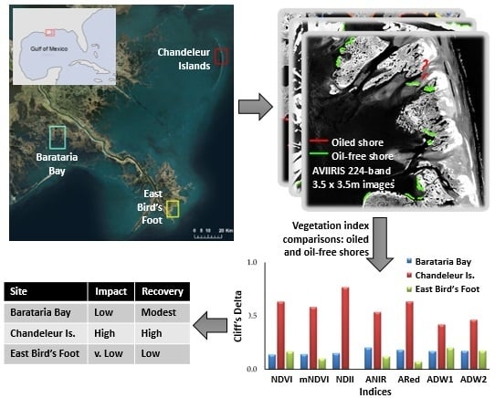
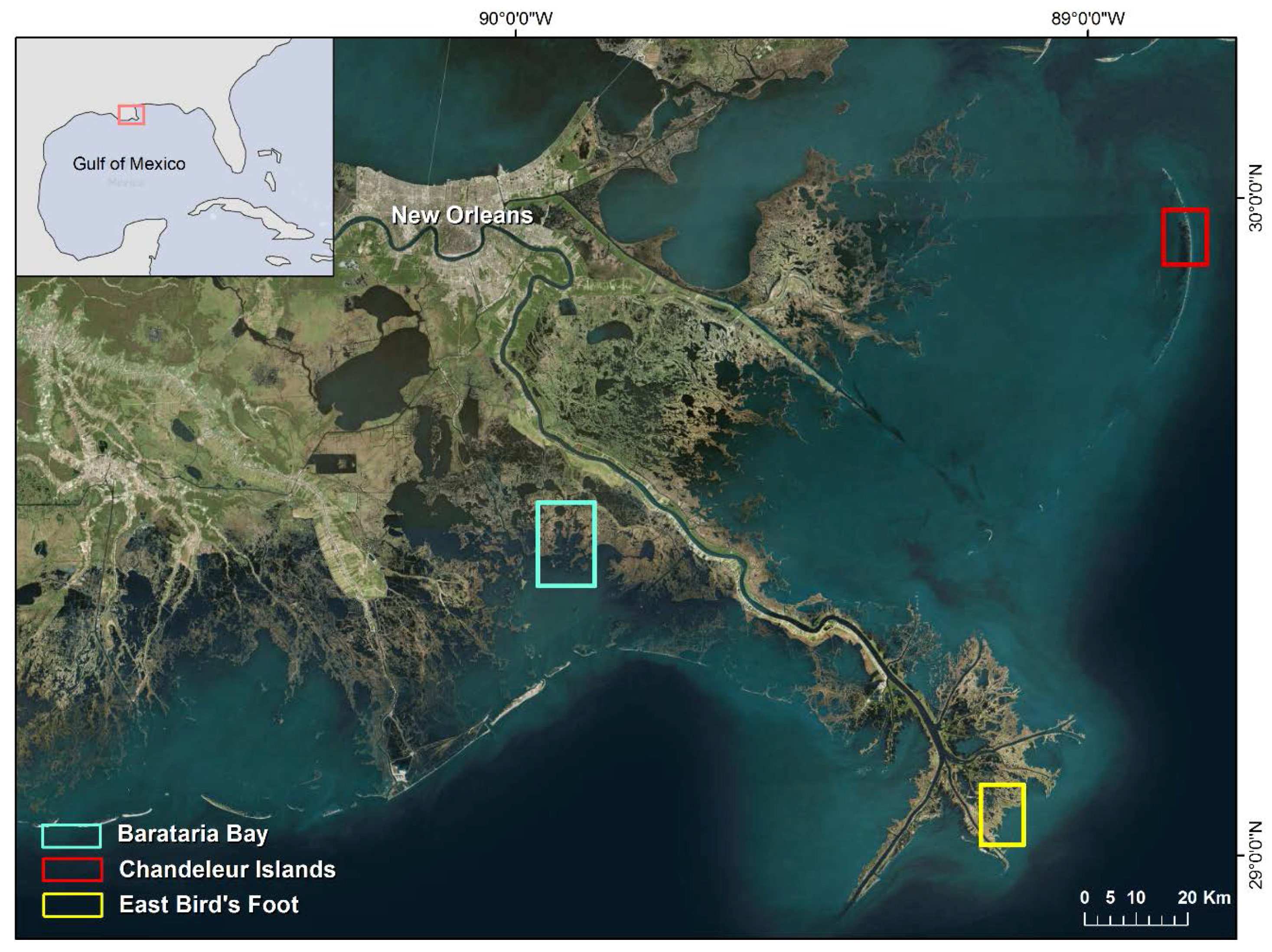
2.1. Study Sites
2.2. Field Data
2.3. Image Data and Preprocessing
2.4. Image Analysis
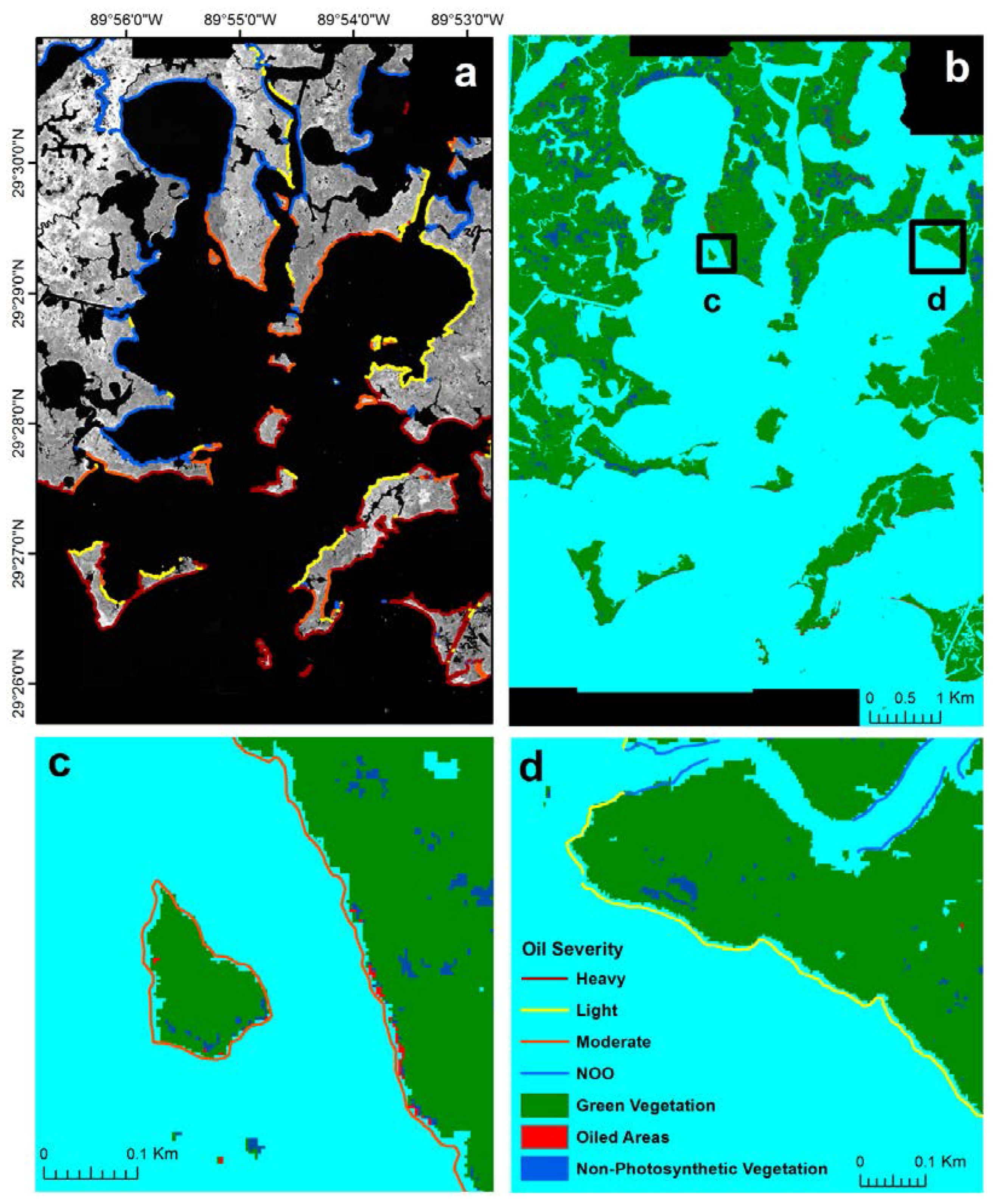
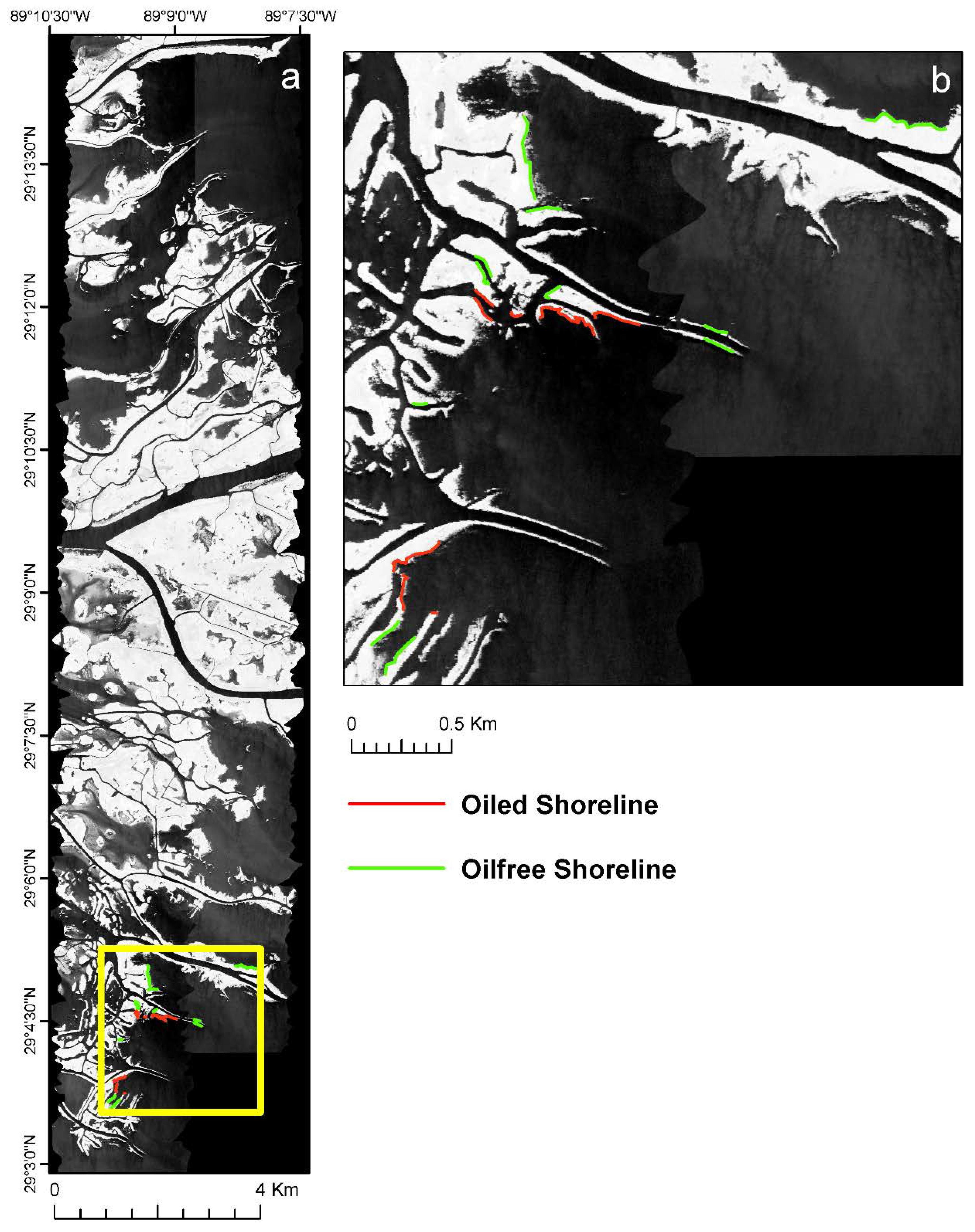
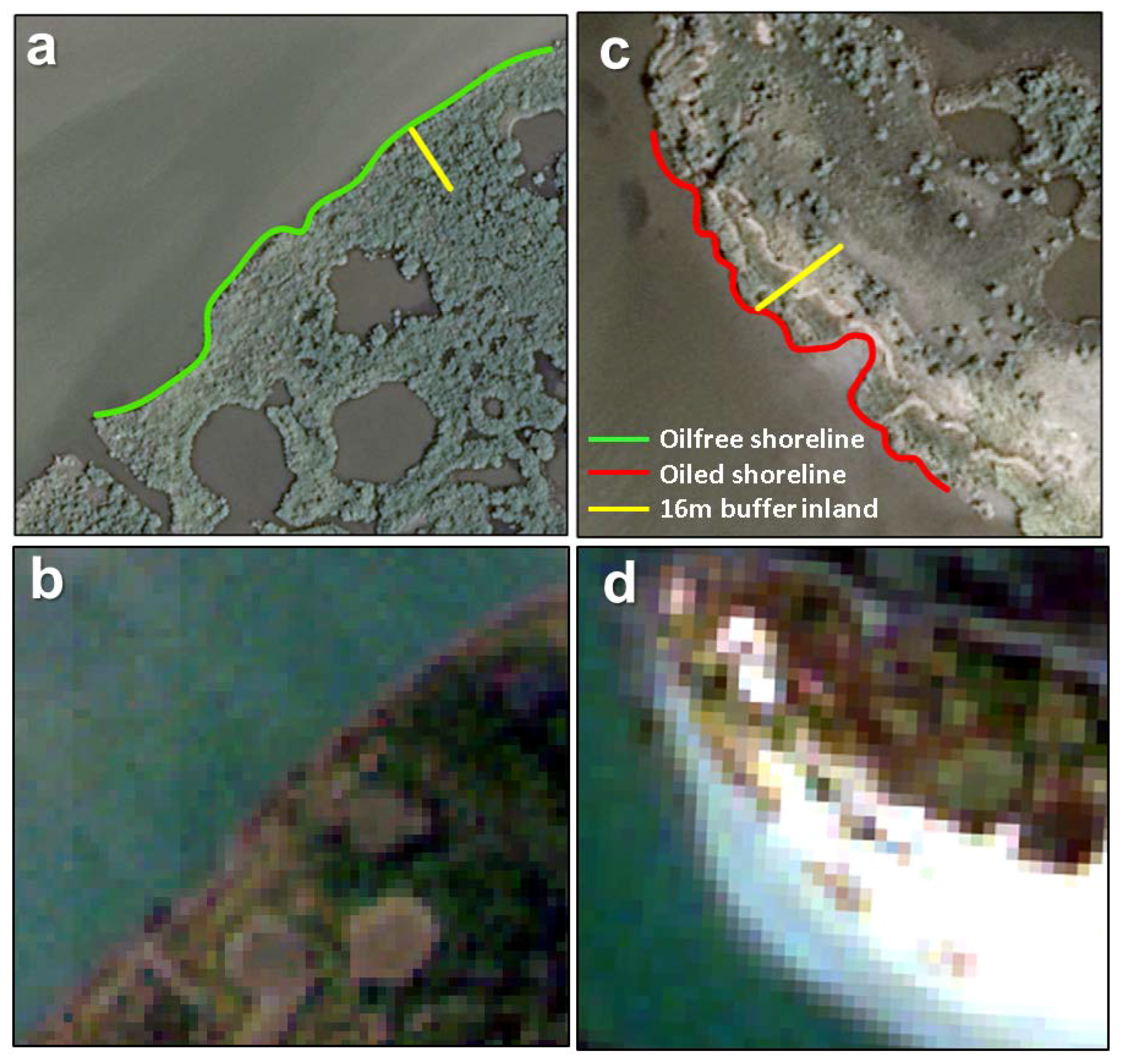
2.4.1. Selection of Oiled and Oil-Free Shores
2.4.2. Comparison of Oil Impact across Sites
2.4.3. Comparison of Recovery from the Oil Spill across Sites
- PCveg2010 = percentage of green vegetation pixels in 2010
- PXveg2010 = total number of pixels of green vegetation in 2010
- PXtotal2010 = total number of pixels analyzed
3. Results
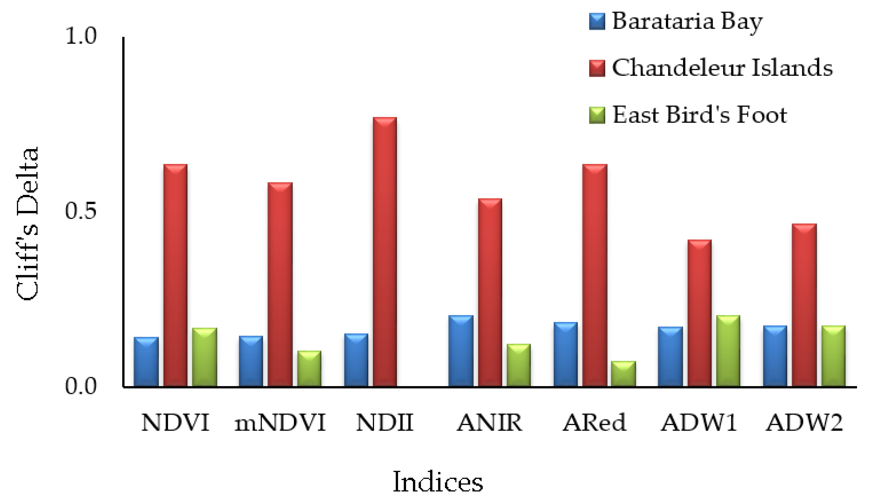
3.1. Comparison of Oil Impact across Sites
3.2. Comparison of Recovery from Oil across Sites
4. Discussion
4.1. Comparison of Oil Impact across Sites
4.2. Comparison of Recovery from Oil across Sites
5. Conclusions
Acknowledgments
Author Contributions
Conflicts of Interest
Abbreviations
| ADW1 | Absorption Depth of Water at 980 nm |
| ADW2 | Absorption Depth of Water at 1240 nm |
| ANIR | Angle formed at NIR |
| ANOVA | ANalysis Of VAriance |
| ARed | Angle formed at Red |
| AVIRIS | Airborne Visible/Infrared Imaging Spectrometer |
| BB | Barataria Bay |
| BP-DWH | British Petroleum—DeepWater Horizon (oil spill) |
| CI | Chandeleur Islands |
| EBF | East Bird’s Foot |
| ERMA | Environmental Response Management Application |
| MDP | Mississippi Deltaic Plain |
| mNDVI | modified Normalized Difference Vegetation Index |
| NASA | National Aeronautics and Space Administration |
| NDII | Normalized Difference Infrared Index |
| NDVI | Normalized Difference Vegetation Index |
| NIR | Near InfraRed |
| NOAA | National Oceanic and Atmospheric Administration |
| NPV | Non-photosynthetic vegetation |
| REIP | Red edge Inflexion Point |
| SCAT | Shoreline Cleanup Assessment Technique |
References
- Wiens, J.A. Review of an ecosystem services approach to assessing the impacts of the Deepwater Horizon Oil Spill in the Gulf of Mexico. Fisheries 2015, 40, 86–86. [Google Scholar] [CrossRef]
- Ko, J.Y.; Day, J.W. A review of ecological impacts of oil and gas development on coastal ecosystems in the Mississippi Delta. Ocean Coast. Manag. 2004, 47, 597–623. [Google Scholar] [CrossRef]
- Gosselink, J.G.; Pendleton, E.C. The Ecology of Delta Marshes of Coastal Louisiana: A Community Profile; U.S. Fish and Wildlife Service: Washington, D.C., USA, 1984; p. 156.
- Couvillion, B.R.; Barras, J.A.; Steyer, G.D.; Sleavin, W.; Fischer, M.; Beck, H.; Trahan, N.; Griffin, B.; Heckman, D. Land Area Change in Coastal Louisiana (1932 to 2010); USGS National Wetlands Research Center: Lafayette, LA, USA, 2011.
- Silliman, B.R.; van de Koppel, J.; McCoy, M.W.; Diller, J.; Kasozi, G.N.; Earl, K.; Adams, P.N.; Zimmerman, A.R. Degradation and resilience in Louisiana salt marshes after the BP-Deepwater Horizon oil spill. Proc. Natl. Acad. Sci. USA 2012, 109, 11234–11239. [Google Scholar] [CrossRef] [PubMed]
- Hester, M.W.; Mendelssohn, I.A. Long-term recovery of a Louisiana brackish marsh plant community from oil-spill impact: Vegetation response and mitigating effects of marsh surface elevation. Mar. Environ. Res. 2000, 49, 233–254. [Google Scholar] [CrossRef]
- Pezeshki, S.R.; Hester, M.W.; Lin, Q.; Nyman, J.A. The effects of oil spill and clean-up on dominant US Gulf coast marsh macrophytes: A review. Environ. Pollut. 2000, 108, 129–139. [Google Scholar] [CrossRef]
- Li, L.; Ustin, S.L.; Lay, M. Application of AVIRIS data in detection of oil-induced vegetation stress and cover change at Jornada, New Mexico. Remote Sens. Environ. 2005, 94, 1–16. [Google Scholar] [CrossRef]
- Horler, D.N.H.; Dockray, M.; Barber, J. The red edge of plant leaf reflectance. Int. J. Remote Sens. 1983, 4, 273–288. [Google Scholar] [CrossRef]
- Gitelson, A.; Merzlyak, M.N. Spectral reflectance changes associated with autumn senescence of Aesculus hippocastanum L. and Acer platanoides L. Leaves. Spectral features and relation to chlorophyll estimation. J. Plant Physiol. 1994, 143, 286–292. [Google Scholar] [CrossRef]
- Tucker, C.J. Red and photographic infrared linear combinations for monitoring vegetation. Remote Sens. Environ. 1979, 8, 127–150. [Google Scholar] [CrossRef]
- Hunt, E.R.; Rock, B.N. Detection of changes in leaf water content using near-infrared and middle-infrared reflectances. Remote Sens. Environ. 1989, 30, 43–54. [Google Scholar]
- Khanna, S.; Santos, M.J.; Ustin, D.S.L.; Koltunov, A.; Kokaly, R.F.; Roberts, D.A. Detection of salt marsh vegetation stress after the Deepwater Horizon BP oil spill along the shoreline of gulf of Mexico using AVIRIS data. PloS ONE 2013, 8, e78989. [Google Scholar] [CrossRef] [PubMed]
- Khanna, S.; Palacios-Orueta, A.; Whiting, M.L.; Ustin, S.L.; Riano, D.; Litago, J. Development of angle indexes for soil moisture estimation, dry matter detection and land-cover discrimination. Remote Sens. Environ. 2007, 109, 154–165. [Google Scholar] [CrossRef]
- Dibner, P.C. Response of A Salt Marsh to Oil Spill and Cleanup: Biotic and Erosional Effects in the Hackensack Meadowlands, New Jersey. Final report, May 1976–December 1977; URS Research Co.: San Mateo, CA, USA, 1978. [Google Scholar]
- Long, B.F.; Vandermeulen, J.H. Geomorphological impact of cleaup of an oiled salt marsh (Ile Grande, France). In Proceedings of the International Oil Spill Conference, San Antonio, Texas, USA, 28 February–3 March 1983; pp. 501–505.
- Mishra, D.R.; Cho, H.J.; Ghosh, S.; Fox, A.; Downs, C.; Merani, P.B.T.; Kirui, P.; Jackson, N.; Mishra, S. Post-spill state of the marsh: Remote estimation of the ecological impact of the Gulf of Mexico oil spill on Louisiana Salt Marshes. Remote Sens. Environ. 2012, 118, 176–185. [Google Scholar] [CrossRef]
- Rosso, P.H.; Pushnik, J.C.; Lay, M.; Ustin, S.L. Reflectance properties and physiological responses of Salicornia virginica to heavy metal and petroleum contamination. Environ. Pollut. 2005, 137, 241–252. [Google Scholar] [CrossRef] [PubMed]
- Van der Meer, F.; van Dijk, P.; van der Werff, H.; Yang, H. Remote sensing and petroleum seepage: A review and case study. Terra Nova 2002, 14, 1–17. [Google Scholar] [CrossRef]
- Yang, H.; Zhang, J.; van der Meer, F.; Kroonenberg, S.B. Geochemistry and field spectrometry for detecting hydrocarbon microseepage. Terra Nova 1998, 10, 231–235. [Google Scholar] [CrossRef]
- Bammel, B.H.; Birnie, R.W. Spectral Reflectance Response of Big Sagebrush to Hydrocarbon-Induced Stress in the Bighorn Basin, Wyoming; American Society for Photogrammetry and Remote Sensing: Bethesda, MD, USA, 1994; Volume 60. [Google Scholar]
- Khanna, S.; Santos, M.J.; Ustin, S.L.; Haverkamp, P.J. An integrated approach to a biophysiologically based classification of floating aquatic macrophytes. Int. J. Remote Sens. 2011, 32, 1067–1094. [Google Scholar] [CrossRef]
- Judy, C.R.; Graham, S.A.; Lin, Q.; Hou, A.; Mendelssohn, I.A. Impacts of Macondo oil from Deepwater Horizon spill on the growth response of the common reed Phragmites australis: A mesocosm study. Mar. Pollut. Bull. 2014, 79, 69–76. [Google Scholar] [CrossRef] [PubMed]
- Lin, Q.; Mendelssohn, I.A. Impacts and recovery of the Deepwater Horizon Oil Spill on vegetation structure and function of coastal salt marshes in the northern gulf of Mexico. Environ. Sci. Technol. 2012, 46, 3737–3743. [Google Scholar] [CrossRef] [PubMed]
- Wu, W.; Biber, P.D.; Peterson, M.S.; Gong, C. Modeling photosynthesis of Spartina alterniflora (smooth cordgrass) impacted by the Deepwater Horizon oil spill using Bayesian inference. Environ. Res. Lett. 2012, 7, 045302. [Google Scholar] [CrossRef]
- Visser, J.; Sasser, C.; Chabreck, R.; Linscombe, R.G. Marsh vegetation types of the Mississippi River Deltaic Plain. Estuaries 1998, 21, 818–828. [Google Scholar] [CrossRef]
- Hymel, M. Monitoring Plan for Chandeleur Islands Marsh Restoration; LDNR/Coastal Restoration and Management: Baton Rouge, LA, USA, 2001; p. 12. [Google Scholar]
- Day, J.; Britsch, L.; Hawes, S.; Shaffer, G.; Reed, D.; Cahoon, D. Pattern and process of land loss in the Mississippi Delta: A Spatial and temporal analysis of wetland habitat change. Estuaries 2000, 23, 425–438. [Google Scholar] [CrossRef]
- Wilson, C.A.; Allison, M.A. An equilibrium profile model for retreating marsh shorelines in southeast Louisiana. Estuar. Coast. Shelf Sci. 2008, 80, 483–494. [Google Scholar] [CrossRef]
- NOAA. Deepwater Horizon Data Integration Visualization Exploration and Reporting Application. Available online: http://dwhdiver.orr.noaa.gov (accessed on 31 January 2016).
- CWPPRA. The Mississippi River Delta Basin. Available online: http://lacoast.gov/new/About/Basin_data/mr/ (accessed on 31 January 2016).
- USGS. Coastwide Reference Monitoring System. Available online: http://lacoast.gov/crms2/ (accessed on 31 January 2016).
- Michel, J.; Owens, E.H.; Zengel, S.; Graham, A.; Nixon, Z.; Allard, T.; Holton, W.; Reimer, P.D.; Lamarche, A.; White, M.; et al. Extent and degree of shoreline oiling: Deepwater Horizon oil spill, Gulf of Mexico, USA. PLoS ONE 2013, 8, e65087. [Google Scholar] [CrossRef] [PubMed]
- Kokaly, R.F.; Heckman, D.; Holloway, J.; Piazza, S.C.; Couvillion, B.R.; Steyer, G.D.; Mills, C.T.; Hoefen, T.M. Shoreline Surveys of Oil-Impacted Marsh in Southern Louisiana, July to August 2010: Open-File Report 2011-1022; USGS Crustal Geophysics and Geochemistry Science Center: Denver, CO, USA, 2011.
- Cretini, K.F.; Visser, J.M.; Krauss, K.W.; Steyer, G.D. CRMS Vegetation Analytical Team Framework: Methods for Collection, Development, and Use of Vegetation Response Variables; USGS National Wetlands Research Center: Lafayette, LA, USA, 2011; p. 60.
- Palacios-Orueta, A.; Khanna, S.; Litago, J.; Whiting, M.L.; Ustin, S.L. Assessment of NDVI and NDWI spectral indices using MODIS time series analysis and development of a new spectral index based on MODIS shortwave infrared bands. In Proceedings of the 1st International Conference of Remote Sensing and Geoinformation Processing, Trier, Germany, 7–9 September 2005.
- Friedl, M.A.; Brodley, C.E. Decision tree classification of land cover from remotely sensed data. Remote Sens. Environ. 1997, 61, 399–409. [Google Scholar] [CrossRef]
- Hickman, J.C. The Jepson Manual: Higher Plants of California; University of California Press: Berkeley, CA, USA, 1993. [Google Scholar]
- Biello, M.; Rust, D.; Watkins, T. Oil laps barrier islands; BP grilled about oil spill at Capitol. Available online: http://www.cnn.com (accessed on 4 May 2010).
- Guillot, C. Oil spill hits gulf coast habitats. Available online: http://news.nationalgeographic.com (accessed on 30 April 2010).
- Strassmann, M. The fight over keeping oil out of Barataria Bay. Available online: http://www.cbsnews.com (accessed on 7 July 2010).
- Ustin, S.L.; Roberts, D.A.; Khanna, S.; Shapiro, K.; Beland, M.; Peterson, S.; Roth, K. Coastal Wetland and Near Shore Ecosystem Impacts from the Gulf of Mexico Deepwater Horizon BP Oil Spill Monitored by NASA's AVIRIS and MASTER Imagers; NASA: Davis, CA, USA, 2014.
- Kokaly, R.F.; Couvillion, B.R.; Holloway, J.M.; Roberts, D.A.; Ustin, S.L.; Peterson, S.H.; Khanna, S.; Piazza, S.C. Spectroscopic remote sensing of the distribution and persistence of oil from the Deepwater Horizon spill in Barataria Bay marshes. Remote Sens. Environ. 2013, 129, 210–230. [Google Scholar] [CrossRef]
- Peterson, S.H.; Roberts, D.A.; Beland, M.; Kokaly, R.F.; Ustin, S.L. Oil detection in the coastal marshes of Louisiana using MESMA applied to band subsets of AVIRIS data. Remote Sens. Environ. 2015, 159, 222–231. [Google Scholar] [CrossRef]
- Mann, H.B.; Whitney, D.R. On a test of whether one of two random variables is stochastically larger than the other. Ann. Math. Stat. 1947, 18, 50–60. [Google Scholar] [CrossRef]
- Macbeth, G.; Razumiejczyk, E.; Ledesma, R.D. Cliff’s Delta Calculator: A non-parametric effect size program for two groups of observations. Univ. Psychol. 2011, 10, 545–555. [Google Scholar]
- Cliff, N. Dominance statistics: Ordinal analyses to answer ordinal questions. Psychol. Bull. 1993, 114, 494–509. [Google Scholar] [CrossRef]
- Romano, J.; Kromrey, J.D.; Coraggio, J.; Skowronek, J.; Devine, L. Exploring methods for evaluating group differences on the NSSE and other surveys: Are the t-test and Cohen’s d indices the most appropriate choices? In Proceedings of the Annual Meeting of the Southern Association for Institutional Research, Arlington, VA, USA, 14–17 October 2006.
- Dai, X.L.; Khorram, S. The effects of image misregistration on the accuracy of remotely sensed change detection. ITGRS 1998, 36, 1566–1577. [Google Scholar]
- Khorram, S.; Biging, G.S.; Chrisman, N.R.; Colby, D.R.; Congalton, R.G.; Dobson, J.E.; Ferguson, R.L.; Goodchild, M.R.; Jensen, J.R.; Mace, T.H. Accuracy Assessment of Remote Sensing Derived Change Detection; American Society of Photogrammetry and Remote Sensing (ASPRS): Bethesda, MD, USA, 1998. [Google Scholar]
- McNemar, Q. Note on the sampling error of the difference between correlated proportions or percentages. Psychometrika 1947, 12, 153–157. [Google Scholar] [CrossRef] [PubMed]
- DeLaune, R.D.; Patrick, W.H., Jr.; Buresh, R.J. Effect of crude oil on a Louisiana Spartina alterniflora salt marsh. Environ. Pollut. 1979, 20, 21–31. [Google Scholar] [CrossRef]
- DeLaune, R.D.; Pezeshki, S.R.; Jugsujinda, A.; Lindau, C.W. Sensitivity of US Gulf of Mexico coastal marsh vegetation to crude oil: Comparison of greenhouse and field responses. Aquat. Ecol. 2003, 37, 351–360. [Google Scholar] [CrossRef]
- Pezeshki, S.R.; DeLaune, R.D. Effect of crude oil on gas exchange functions of Juncus roemerianus and Spartina alterniflora. Water Air Soil Pollut. 1993, 68, 461–468. [Google Scholar] [CrossRef]
- Kirby, C.J.; Gosselink, J.G. Primary Production in a Louisiana Gulf Coast Spartina Alterniflora Marsh. Ecology 1976, 57, 1052–1059. [Google Scholar] [CrossRef]
- Hoff, R.; Hensel, P.; Proffitt, E.C.; Delgado, P.; Shigenaka, G.; Yender, R.; Mearns, A.J. Oil Spills in Mangroves: Planning & Response Considerations; U.S. Department of Commerce, NOAA: Seattle, WA, USA, 2010; p. 72.
- Hester, M.W.; Spalding, E.A.; Franze, C.D. Biological resources of the Louisiana Coast: Part 1. An overview of coastal plant communities of the Louisiana gulf shoreline. J. Coast. Res. 2005, 134–145. Available online: http://www.jstor.org/stable/25737053 (accessed on 22 April 2016). [Google Scholar]
- Dowty, R.A.; Shaffer, G.P.; Hester, M.W.; Childers, G.W.; Campo, F.M.; Greene, M.C. Phytoremediation of small-scale oil spills in fresh marsh environments: A mesocosm simulation. Mar. Environ. Res. 2001, 52, 195–211. [Google Scholar] [CrossRef]
- Lin, Q.; Mendelssohn, I.A.; Hester, M.W.; Webb, E.C.; Henry, J.; Charles, B. Effect of oil cleanup methods on ecological recovery and oil degradation of Phragmites marshes. Int. Oil Spill Conf. Proc. 1999, 1999, 511–517. [Google Scholar] [CrossRef]
- Armstrong, J.; Keep, R.; Armstrong, W. Effects of oil on internal gas transport, radial oxygen loss, gas films and bud growth in Phragmites australis. Ann. Bot. 2009, 103, 333–340. [Google Scholar] [CrossRef]
- DeLaune, R.D.; Wright, A.L. Projected impact of Deepwater Horizon oil spill on U.S. gulf coast wetlands. Soil Sci. Soc. Am. J. 2011, 75, 1602–1612. [Google Scholar] [CrossRef]
- Smith, C.J.; Delaune, R.D.; Patrick, W.H.; Fleeger, J.W. Impact of dispersed and undispersed oil entering a gulf coast salt marsh. Environ. Toxicol. Chem. 1984, 3, 609–616. [Google Scholar] [CrossRef]
- Hayden, B.P.; Santos, M.C.F.V.; Shao, G.; Kochel, R.C. Geomorphological controls on coastal vegetation at the Virginia Coast Reserve. Geomo 1995, 13, 283–300. [Google Scholar] [CrossRef]
- Grant, D.L.; Clarke, P.J.; Allaway, W.G. The response of grey mangrove (Avicennia marina (Forsk.) Vierh.) seedlings to spills of crude oil. J. Exp. Mar. Biol. Ecol. 1993, 171, 273–295. [Google Scholar] [CrossRef]


| Site | Year | Flight Dates | Pixel Resolution (m) | # Flightlines | Water Level (m) | Shoreline Analyzed (km) |
|---|---|---|---|---|---|---|
| BB | 2010 | 09/14 | 3.5 × 3.5 | 4 | 0.21 | 30.4 |
| 2011 | 08/25 | 7.7 × 7.7 | 2 | 0.25 | ||
| CI | 2010 | 09/21 | 3.4 × 3.4 | 2 | 0.66 | 3.2 |
| 2011 | 08/11 | 7.7 × 7.7 | 2 | 0.25 | ||
| EBF | 2010 | 10/03 | 3.4 × 3.4 | 2 | 0.11 | 4.3 |
| 2011 | 10/14 | 3.4 × 3.4 | 2 | 0.18 |
| Acronym | Formula | Plant | References |
|---|---|---|---|
| NDVI | (RNIR − RR)/(RNIR + RR) | chlorophyll content and/or leaf area of the plant | [11] |
| mNDVI | (R750 − R700)/(R750 + R700) | chlorophyll content and/or leaf area of the plant | [10] |
| NDII | (RNIR − R923)/(RNIR + R923) | Water content | [12] |
| ANIR | Angle between (RR, λR), (RNIR, λNIR), and (RSWIR, λSWIR) | Phenology and stress | [14,36] |
| ARed | Angle between (RR, λR), (RR, λR), and (RNIR, λNIR) | Phenology and stress | [13,36] |
| ADW1 | 0.5 × (R1070 + R890) − R990 | Water content | [13] |
| ADW2 | 0.5 × (R1270 + R1070) − R1167 | Water content | [13] |
| Site | Median | U | p-Value | Cliff’s Delta | |
|---|---|---|---|---|---|
| Oiled | Oil-Free | ||||
| BB | n = 36,588 | n = 23,319 | |||
| NDVI | 0.61 | 0.68 | 366,505,856 | <0.0001 | 0.14 |
| mNDVI | 0.30 | 0.37 | 365,362,851 | <0.0001 | 0.14 |
| NDII | 0.20 | 0.24 | 361,584,380 | <0.0001 | 0.15 |
| ANIR | 0.95 | 0.50 | 513,898,843 | <0.0001 | 0.20 |
| ARed | 4.67 | 4.99 | 348,463,947 | <0.0001 | 0.18 |
| ADW1 | 219.62 | 270.51 | 353,379,597 | <0.0001 | 0.17 |
| ADW2 | 414.13 | 484.95 | 352,463,292 | <0.0001 | 0.17 |
| CI | n = 3,089 | n = 8,460 | |||
| NDVI | 0.31 | 0.55 | 4,782,283 | <0.0001 | 0.63 |
| mNDVI | 0.11 | 0.28 | 5,436,240 | <0.0001 | 0.58 |
| NDII | 0.10 | 0.36 | 3,023,503 | <0.0001 | 0.77 |
| ANIR | 1.56 | 0.70 | 20,080,843 | <0.0001 | 0.54 |
| ARed | 4.71 | 5.56 | 4,765,186 | <0.0001 | 0.64 |
| ADW1 | 249.26 | 425.32 | 7,584,217 | <0.0001 | 0.42 |
| ADW2 | 374.55 | 621.53 | 7,011,257 | <0.0001 | 0.46 |
| EBF | n = 1,620 | n = 2,982 | |||
| NDVI | 3.5 | 0.81 | 2,822,096 | <0.0001 | 0.17 |
| mNDVI | 0.68 | 0.68 | 2,663,718 | <0.0001 | 0.10 |
| NDII | 0.63 | 0.63 | 2,428,518 | 0.7600 | - |
| ANIR | 0.23 | 0.22 | 2,122,563 | <0.0001 | 0.12 |
| ARed | 5.98 | 5.98 | 2,592,410 | 0.0007 | 0.07 |
| ADW1 | 438.40 | 510.04 | 2,905,034 | <0.0001 | 0.20 |
| ADW2 | 478.29 | 543.92 | 2,839,563 | <0.0001 | 0.18 |
| Class | Barataria Bay | Chandeleur Islands | East Bird’s Foot | |||
|---|---|---|---|---|---|---|
| 2010 | 2011 | 2010 | 2011 | 2010 | 2011 | |
| Green Vegetation | 199,985 | 278,078 | 9,724 | 20,455 | 29,351 | 31,015 |
| NPV-Soil | 69,191 | 14,763 | 9,071 | 10,672 | 913 | 208 |
| Water | 309,375 | 285,719 | 12,629 | 296 | 33,050 | 32,091 |
| PCveg | 34.6% | 48.1% | 30.9% | 65.1% | 46.4% | 49.0% |
© 2016 by the authors; licensee MDPI, Basel, Switzerland. This article is an open access article distributed under the terms and conditions of the Creative Commons Attribution license ( http://creativecommons.org/licenses/by/4.0/).
Share and Cite
Shapiro, K.; Khanna, S.; Ustin, S.L. Vegetation Impact and Recovery from Oil-Induced Stress on Three Ecologically Distinct Wetland Sites in the Gulf of Mexico. J. Mar. Sci. Eng. 2016, 4, 33. https://doi.org/10.3390/jmse4020033
Shapiro K, Khanna S, Ustin SL. Vegetation Impact and Recovery from Oil-Induced Stress on Three Ecologically Distinct Wetland Sites in the Gulf of Mexico. Journal of Marine Science and Engineering. 2016; 4(2):33. https://doi.org/10.3390/jmse4020033
Chicago/Turabian StyleShapiro, Kristen, Shruti Khanna, and Susan L. Ustin. 2016. "Vegetation Impact and Recovery from Oil-Induced Stress on Three Ecologically Distinct Wetland Sites in the Gulf of Mexico" Journal of Marine Science and Engineering 4, no. 2: 33. https://doi.org/10.3390/jmse4020033