Article

Construction of a Static Model for Power Generation of OTEC Plant Using Uehara Cycle Based on Experimental Data

1
Graduate School of Science and Engineering, Saga University, 1 Honjo-machi, Saga 840-8502, Japan
2
Institute of Ocean Energy, Saga University, 1 Honjo-machi, Saga 840-8502, Japan
*
Author to whom correspondence should be addressed.
J. Mar. Sci. Eng. 2018, 6(1), 18; https://doi.org/10.3390/jmse6010018
Submission received: 28 December 2017 / Revised: 2 February 2018 / Accepted: 12 February 2018 / Published: 15 February 2018
(This article belongs to the Special Issue Ocean Thermal Energy Conversion)

Abstract

:
This paper considers the construction of a static model for the power generation of an ocean thermal energy conversion (OTEC) plant using Uehara cycle. The model is constructed based on experimental data obtained from an actual experimental OTEC plant. In this paper, two kinds of static models are proposed. In both models, the relations among significant quantities are represented by polynomials. The polynomials are determined via least squares for experimental data, and the orders of polynomial which minimize the integral of absolute error between experimental data and simulation results of power generation are adopted. The usefulness and limitations of the proposed models are evaluated by simulation results.

1. Introduction

Ocean thermal energy conversion (OTEC) [1] is one of the power generation methods which bring renewable energy. OTEC is the system which realizes the power generation by using the temperature difference between surface warm seawater and deep-sea cold seawater. OTEC technology provides the following preferable features: The heat source is semi-permanently available since warm seawater (25–30 C) and cold seawater (5–10 C) are used as the heat source. The OTEC plant does not emit CO 2 during operation since fossil fuels such as coal are not used. Furthermore, the integration of the OTEC technology with deep seawater and/or the desalination of seawater [2,3,4,5,6,7] can be realized. In [2], dual-use open cycle OTEC using multiple condensers for adjustable power generation and seawater desalination was investigated from the theoretical point of view. In [3], an integrated multigeneration system with desalination by using renewable energies was proposed. In [4], an experimental study on a spray flash desalination to evaluate the influence of the direction of injection was conducted. In [5], the design method and experimental results for an experimental spray flash desalination apparatus were discussed. In [6], an experimental study of spray flash evaporation for an OTEC plant using an integrated hybrid OTEC cycle and desalination was conducted. In [7], a simulation model for spray flash desalination system was constructed based on the mass and energy conservation laws. For the practical development of OTEC technology, some researches on the oceanic and potential investigations for the OTEC plant construction [8,9,10,11,12,13,14,15,16], cycles and heat exchangers [17,18,19,20,21,22,23,24], at-sea experiments [25], and so on have been conducted. In [8], the distribution of Florida’s OTEC resource was assessed. In [9], OTEC potential in the Indonesian seas was investigated. In [10], global OTEC resources were estimated by using an ocean general circulation model. In [11], the technical, economic, environmental and resource factors of OTEC research in Japan are summarized. In [12], 14 suitable sites in the Philippine seas and the conceptual design of OTEC plants were proposed. In [13], the current status and future prospects in Malaysia for five types of ocean renewable energy including OTEC were reviewed. In [14], the investigation results of marine meteorology carried out off the coast of the Oki-no-Erabu island for OTEC by using a training ship were summarized. In [15], the energy source investigation results in five seas for OTEC were shown. In [16], the results obtained from the oceangraphic observations off the coast of Fiji Island were given. In [17], the performance of an OTEC plant using an organic Rankine cycle was analyzed. In [18], the optimization design and exergy analysis of OTEC plant using organic Rankine cycle were considered. In [19], the comparison of experimental results from an OTEC experimental plant using double-stage Rankine cycle with theoretical ones were carried out. In [20], a transient model of OTEC plant using Rankine cycle was constructed through experimental investigations. In [21,22], performance tests of a shell and plate type condenser and evaporator for OTEC were reported, respectively. In [23], the controller design for vapor temperatures of OTEC plant using Rankine cycle was considered based on a reduced order model. In [24], the results of the performance test of OTEC with ammonia water mixture using shell and plate type heat exchangers were evaluated. In [25], at-sea experiments of an OTEC experimental facility in Toyama Bay were carried out.
In general, the thermal efficiency of OTEC plants is relatively low compared with that of thermal power plants etc. since the temperature difference between warm and cold seawater is small (about 20 C). To realize the power generation by the low temperature difference, Kalina cycle [26] was proposed which uses ammonia/water mixture as the working fluid. In the Kalina cycle, the cycle thermal efficiency was improved by utilizing the evaporating and condensing temperatures of the mixture. In order to obtain higher thermal efficiency, Uehara cycle [27,28] was proposed by using two turbines and introducing absorption and extraction to Kalina cycle. For the controller design and simulator development, a model for OTEC plant using Uehara cycle was developed [29]. The model was constructed based on the mass balance and the heat balance. In the model construction, a program package for thermophysical properties of fluid (PROPATH) [30] was used for the calculation of thermophysical properties of ammonia/water mixture. However, the model takes significant computational time to carry out simulations by the model and the range of working fluid mass flow rate to be able to conduct simulations successfully is limited.
In this paper, a static model for the power generation of OTEC plant using Uehara cycle is proposed to not only represent the characteristics of the plant appropriately but also to realize reasonable computational time for simulations. The model is constructed via least squares for experimental data of an actual OTEC experimental plant. The usefulness of the proposed methodology is verified by numerical simulations.

2. OTEC Plant Using Uehara Cycle

The structure of an OTEC experimental plant using Uehara cycle at the Institute of Ocean Energy, Saga University, Saga, Japan (IOES) [31] is shown in Figure 1. The principal components are an evaporator, a condenser, a separator, two turbines, a generator, an absorber, two tanks, two working fluid pumps, a regenerator, a heater and a diffuser. The use of ammonia/water mixture as the working fluid is one of the remarkable characteristics of OTEC plant using Uehara cycle, which is introduced to realize higher thermal efficiency. Furthermore, Uehara cycle has two turbines to extract unused heat energy.
Part of working fluid is changed from liquid to vapor in the evaporator by the heat exchange for the warm water, where the working fluid is sent to the evaporator by the working fluid pump 1 after passing through the heater and the regenerator. The working fluid is separated into vapor and liquid in the separator. The vapor is sent to turbine 1 to do the work of rotating turbine 1, where part of the vapor is extracted and sent to the heater. The rest of the vapor does the work of rotating turbine 2 and is sent to the absorber. The electricity is generated by the generator connected to the turbines. The liquid of working fluid separated in the separator is sent to the regenerator to heat the working fluid sent to the evaporator. Then, the liquid of working fluid is sent to the absorber. The vapor and liquid sent to the absorber are completely condensed in the condenser by the heat exchange for the cold water. The working fluid extracted from turbine 1 heats the working fluid sent from tank 1 to the evaporator and joins it at the outlet of the working fluid pump 2. The power generation is performed by repeating the above procedure.
In [29], a model for numerical simulation of OTEC plant using Uehara cycle was constructed based on the mass conservation law and the energy conservation law. It uses a software package PROPATH for the thermophysical properties of ammonia/water mixture. The model consists of a condenser part (condenser, tank 1, absorber, working fluid pump 1), a heater part (heater, tank 2, working fluid pump 2), a regenerator, an evaporator part (evaporator, separator), a turbine part (turbine 1, turbine 2, generator) and a diffuser. It is represented by 54 relations (11 relations for condenser part, 5 for heater part, 6 for regenerator, 14 for evaporator part, 15 for turbine part, and 3 for diffuser) and calculates the working fluid flow rates, the enthalpies, the heat flow rates, the temperatures, the pressures, the specific volumes, the mass fractions, the overall heat transfer coefficients and the power generation. The outlet condenser temperature is calculated under the condition that overall heat transfer coefficients represented in two ways equal. The problem of calculating the temperature is reduced to that of solving a nonlinear algebraic equation iteratively. However, this problem causes heavy computational burden, where the convergence is also not guaranteed. The numerical simulations for the verification of the model were conducted in [29]. However, the applicable range of working fluid flow rate is limited near the neighborhood of the rated power output (30 kW). Indeed, in the numerical simulations for the working fluid flow rates out of the applicable range, the calculation does not converge successfully. Furthermore, it is difficult to resolve this problem due to the complexity of the model which comes from the complicated structure of Uehara cycle.
Thus, in this paper, a novel methodology for the construction of a model of OTEC plant using Uehara cycle based on experimental data is proposed to solve the problems pertaining to the applicable working fluid flow rate and the computational burden.

3. Construction of Static Model for Power Generation

In this paper, a model is constructed based on experimental data for the steady state, where the data are obtained from OTEC experimental equipment using Uehara cycle. In experiments using the experimental equipment, quantities such as the pressure P, the flow rate m ˙ , the power output G T B etc. are measured by instruments located at the inlet and outlet of each component. They are recorded at every constant time interval ( 10 s in this paper). The inlet-outlet relations of each component are determined based on the experimental data. The performance evaluation of the OTEC experimental plant for steady state is usually conducted by changing the working fluid flow rate m ˙ L I P M 1 through the operation of working fluid pump 1 in Figure 1 during the experiment. Therefore, in this paper, models with the working fluid flow rate m ˙ L I P M 1 as the input and the power output G T B as the output are constructed, where two kinds of models called warm source side model and cold source side model are proposed. The two models realize the calculations of not only significant quantities for the performance evaluation of OTEC plant but also power output from the viewpoints of warm source side and cold source side. In the construction of the warm source side model, experimental data of working fluid pump 1, the evaporator, the separator and turbine 2 are used. On the other hand, in the construction of the cold source side model, experimental data of working fluid pump 1, turbine 1, the turbine 2, the absorber and the condenser are used. As explained above, in this paper, the model construction is divided into warm source side and cold source side different from the conventional model [29]. By this idea, the difficult problem of the iterative computation of the conventional model can be avoided.
First, averages of inlet and outlet experimental data (or their differences) of each component for some working fluid rates m ˙ L I P M 1 (= 1.67 , 1.94 , 2.22 , 2.50 , 2.78 , 3.33 kg/s in this paper) are calculated, where the average operation is performed to suppress the influence of the measurement noise. Then, the relations among the averages are derived by selecting the explanatory variable x and the objective variable y appropriately via least squares for polynomial approximation (i.e., y = f ( x ) = a 0 + a 1 x + + a k x k ). The order k of polynomials are determined so as to minimize the integral of absolute error (IAE)
J [ t s , t e ] = t s t e | G exp T B ( t ) G T B ( t ) | d t
between the experimental data G exp T B ( t ) and the simulation result G T B ( t ) of power generation, which evaluates the fitness of constructed model for experimental data.

3.1. Heat Source Side Model

In the heat source side model construction, a model about heat source side (inlet and outlet of working fluid pump 1, inlet and outlet of evaporator, separator, outlet of turbine, and generator) is derived to calculate power generation (see warm source side model in Figure 2):
P L I P M 1 = f W 1 ( m ˙ L I P M 1 )
P L O P M 1 = P L I P M 1 + f W 2 ( m ˙ L I P M 1 )
P I E V = P L O P M 1 + f W 3 ( m ˙ L I P M 1 )
P O E V = P I E V + f W 4 ( m ˙ L I P M 1 )
m ˙ V O S P = f W 5 ( P O E V )
P O T B = P O E V + f W 6 ( m ˙ V O S P )
G T B = f W 7 ( P O E V P O T B ) ,
where f W 1 , f W 2 , …, f W 7 are polynomials to be determined, P L I P M 1 is the pressure of working fluid pump inlet, P L O P M 1 is the pressure of working fluid pump outlet, P I E V is the pressure of evaporator inlet, P O E V is the pressure of evaporator outlet, m ˙ V O S P is the vapor flow rate of separator outlet and P O T B is the pressure of turbine outlet.

3.2. Cold Source Side Model

In the cold source side model construction, a model about cold source side (inlet of working fluid pump 1, inlet and outlet of condenser, inlet and outlet of turbine, and generator) is derived to calculate power generation (see cold source side model in Figure 2):
P L I P M 1 = f C 1 ( m ˙ L I P M 1 )
P L O C O = P L I P M 1 + f C 2 ( m ˙ L I P M 1 )
P I C O = P L O C O + f C 3 ( m ˙ L I P M 1 )
m ˙ O T B = f C 4 ( P I C O )
P I T B = P I C O + f C 5 ( m ˙ O T B )
G T B = f C 6 ( P I T B P I C O ) ,
where f C 1 , f C 2 , …, f C 6 are polynomials to be determined, P L O C O is the pressure of condenser outlet, P I C O is the pressure of condenser inlet, m ˙ O T B is the working fluid flow rate of turbine outlet and P I T B is the pressure of turbine inlet.

4. Evaluation by Numerical Simulation

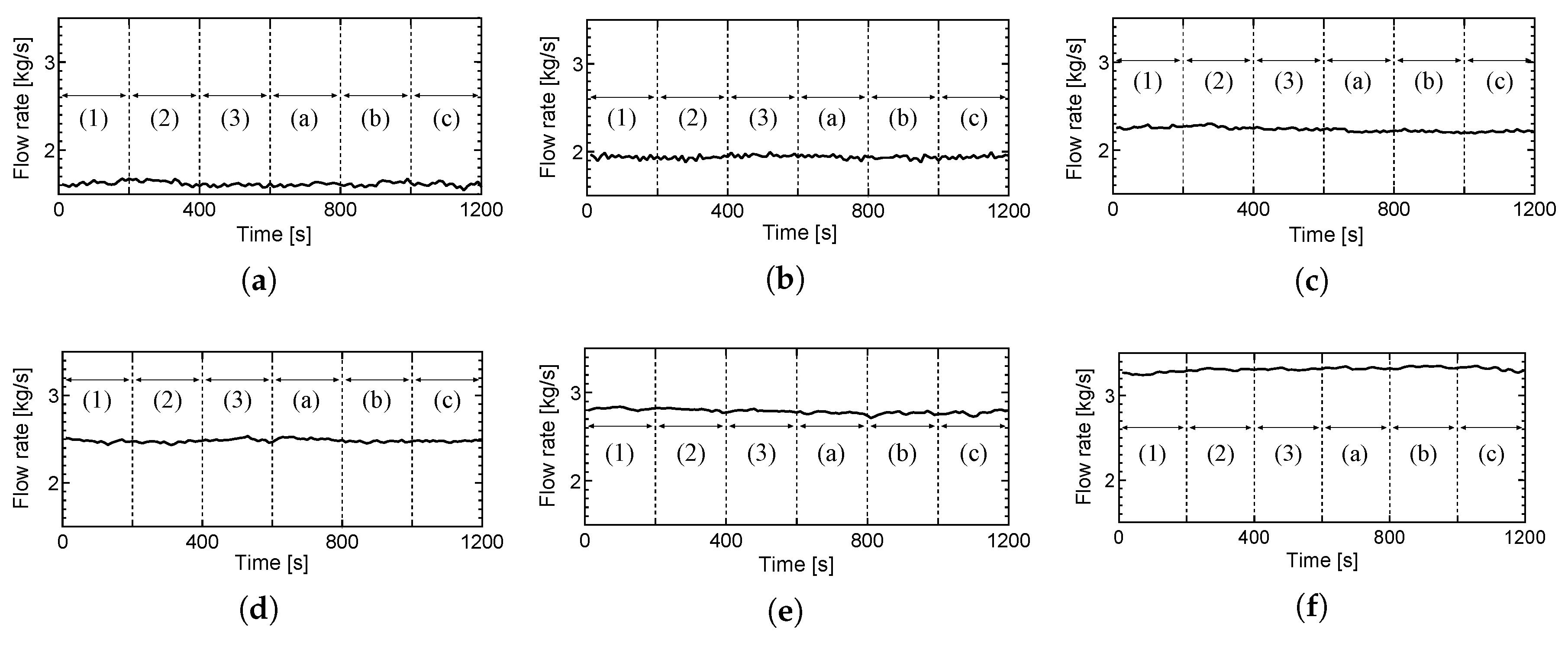
In order to evaluate the usefulness and limitation of the proposed methodology, models were constructed based on experimental data obtained from the OTEC experimental plant using Uehara cycle at IOES and simulations by the models were conducted. The experimental condition is listed in Table 1. The obtained experimental data of working fluid flow rate and power generation are shown in Figure 3 and Figure 4, respectively.

4.1. Derivation of Input-Output Relations

The input-output relations f W 1 , …, f W 7 for warm source side model and f C 1 , …, f C 6 for cold source side model were derived based on the proposed methodology for the construction of power generation static models.
For the derivation of input-output relations, three sets of experimental data corresponding to three intervals (1), (2) and (3) in Figure 3 and Figure 4 were used. By using the data, three models for warm source side and three models for cold source side were constructed. The orders of polynomials ( f W 1 , …, f W 7 for warm source side model; f C 1 , …, f C 6 for cold source side model) were determined so as to minimize IAE Equation (1) by carrying out simulations for all orders. The results are listed in Table 2.
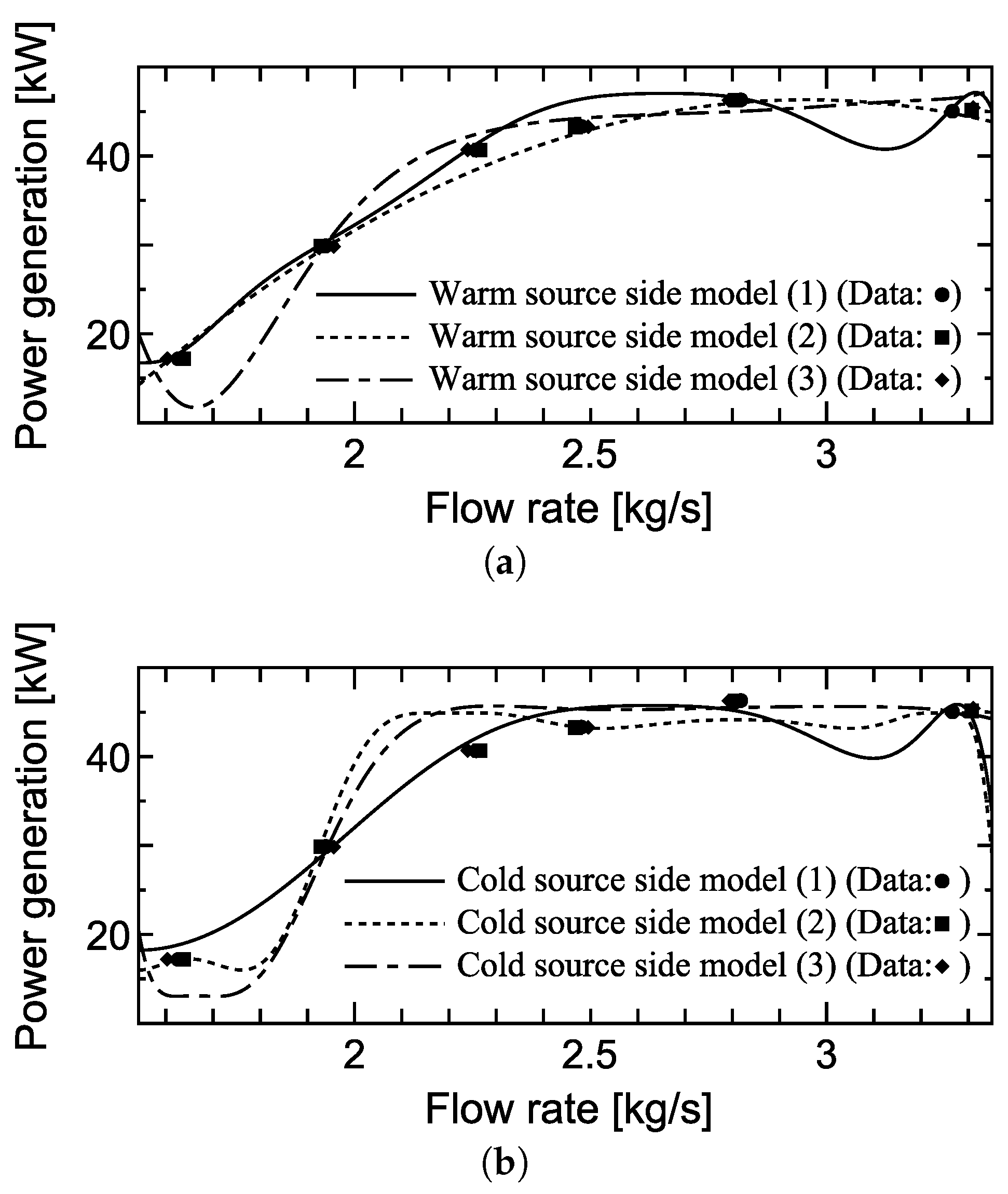
Furthermore, the calculation results of power generation G T B for working fluid flow rate m ˙ L I P M 1 from 1.542 kg/s to 3.350 kg/s by using the obtained models are depicted in Figure 5, where Figure 5a,b are the results for warm and cold source side models, respectively. Table 2 indicates that the orders of polynomials are different if the interval of experimental data to be used is different. One of the reasons that the difference of the orders occurred is the influence of phenomena which have never been described by conventional models. For example, in actual experiments, ripples in the working fluid whose state is the mixture of vapor and liquid at the inlet of the condenser are sometimes generated. Then, the flow rate, the pressure etc. of the working fluid at each component are affected by the ripples even if the behavior of the plant is steady state (or the power output can be regarded as constant). Therefore, to understand the meaning of the differences of the polynomial orders completely, such phenomena must be clarified sufficiently. Furthermore, although both the explanatory variable and the objective variable of relations Equations (2) and (9) are the same, the orders of polynomials are different for data (1)–(3) as shown in Table 2. This difference of orders comes from the minimization of IAE Equation (1).

4.2. Numerical Simulations by Using Experimental Data as Input

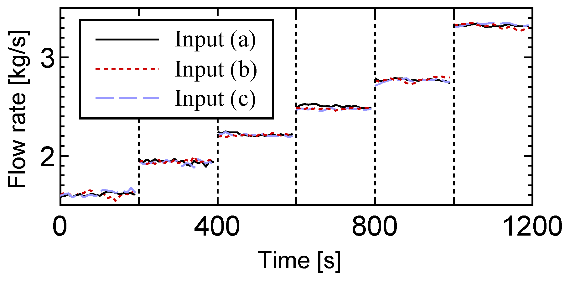
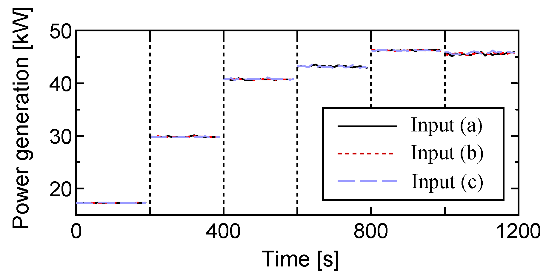
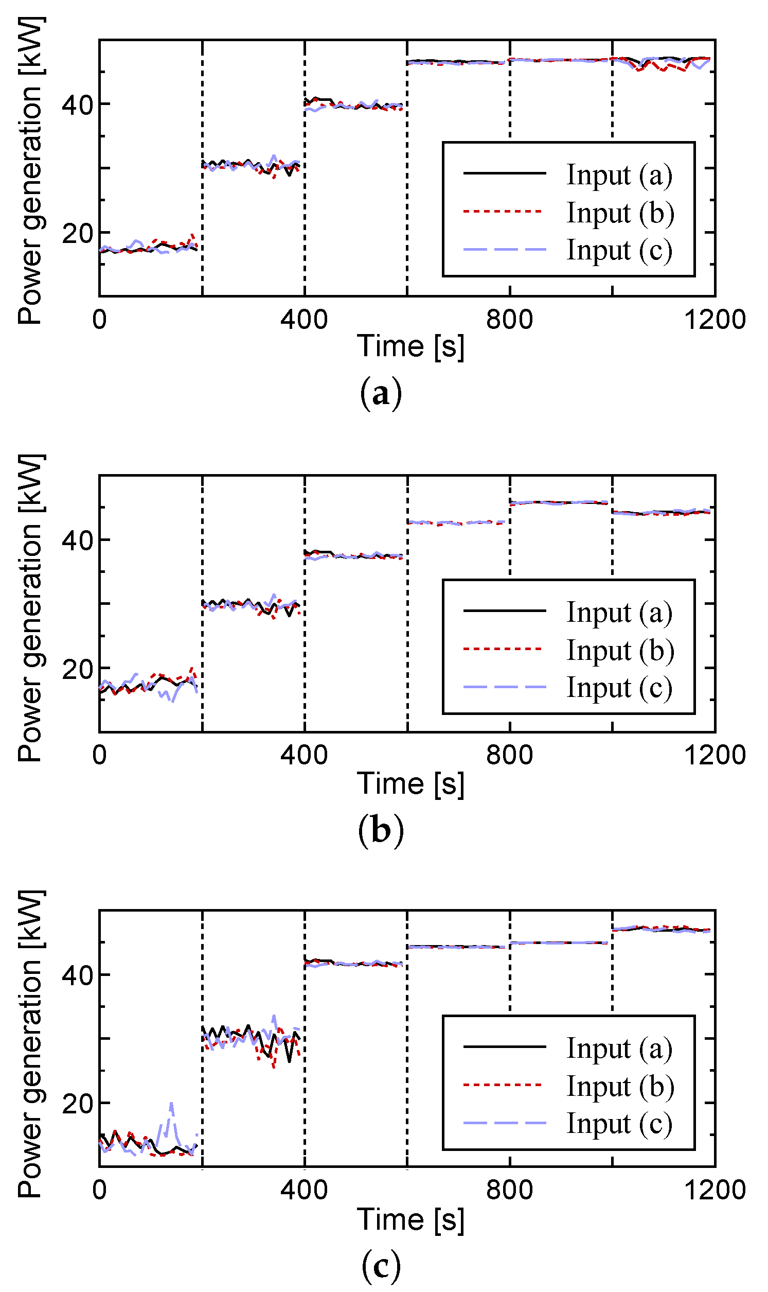
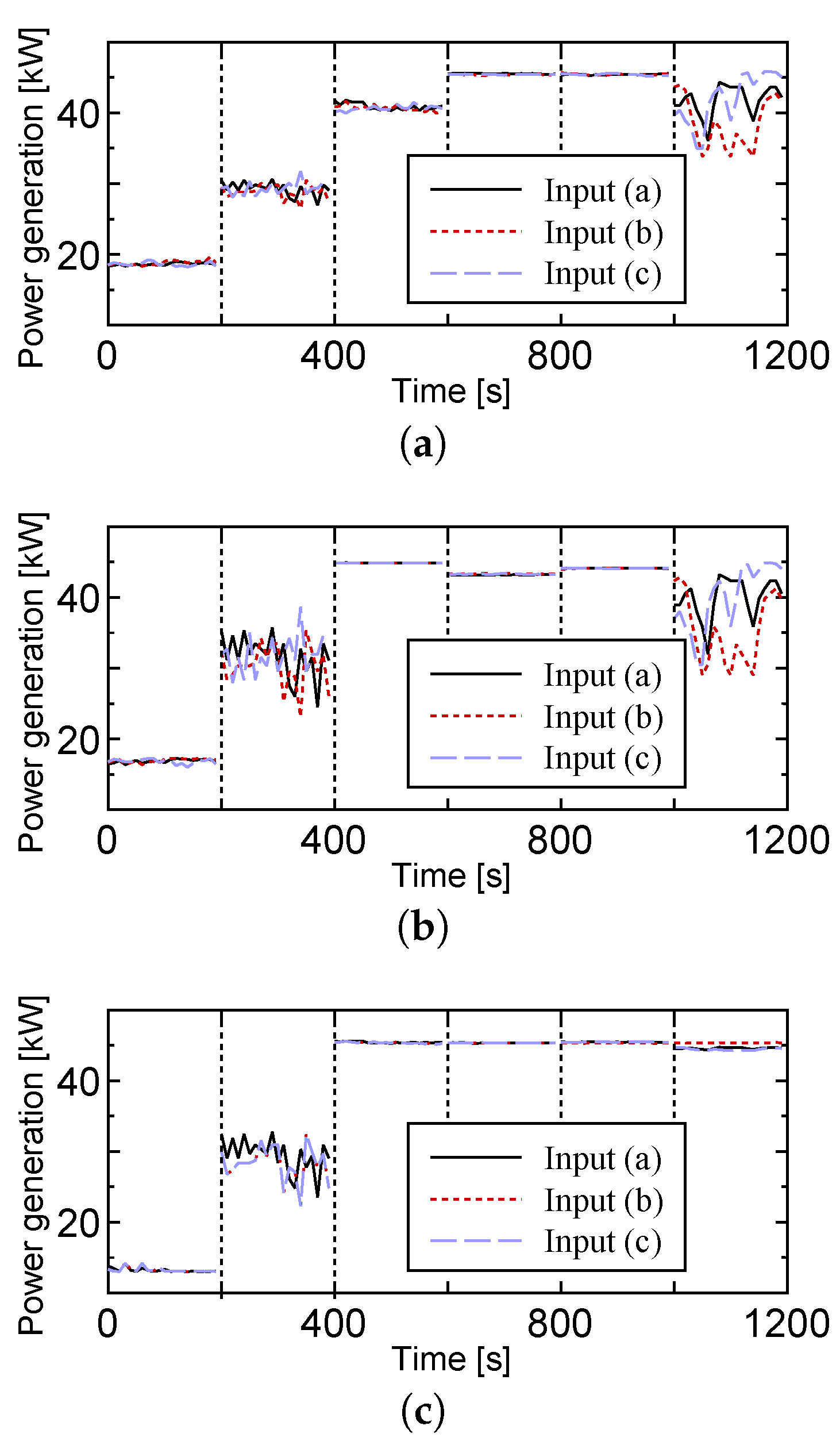
In order to verify the behavior of the constructed models for another experimental data, some simulations were also carried out. For the simulations, three kinds of data for inputs m ˙ L I P M 1 ( t ) and outputs G exp T B ( t ) shown in Figure 6 and Figure 7 corresponding to intervals (a–c) in Figure 3 and Figure 4 were prepared by simply arranging six sets of data in Figure 3 and Figure 4, where as the starting time, t = 0 s, 200 s, 400 s, 600 s, 800 s and 1000 s were assigned for six sets of experimental data from Figure 3 and Figure 4, respectively. Therefore, the simulation results in this subsection are not for dynamic responses but for static ones. Simulation results by warm source side models and cold source side models with inputs (a–c) in Figure 6 are shown in Figure 8 and Figure 9, respectively. Furthermore, the calculation results of IAE between the experimental data G exp T B ( t ) and the simulation result G T B ( t ) in Figure 8 and Figure 9 are listed in Table 3 and Table 4, respectively.
The whole comparison between simulation results in Figure 8 and Figure 9 and experimental data in Figure 7 indicates that almost all of the simulation results have similar behavior to experimental data.
First, let us verify the behavior of each model for three kinds of inputs (i.e., Inputs (a)–(c)). From simulation results in Figure 8 and Figure 9, we see that almost the same outputs except for some time intervals with relatively large variation can be obtained for the same model even if the input data is different. This fact implies that each model strictly captures the phenomena caused in the plant during the acquisition of experimental data and definitely represents the captured phenomena for any inputs.
Secondly, let us check the difference between obtained models. In time intervals 0–400 s of Figure 8 and 200–400 s, 1000–1200 s of Figure 9, the variation of the outputs affected by the variations of inputs are relatively large compared with the other time intervals. Although the magnitude of variations varies with the model, this comes from the difference of polynomial order. Indeed, the output G T B rapidly changes near the working fluid flow rates m ˙ L I P M 1 = 1.6 2.0 kg/s for the warm source side model (3) in Figure 5a, m ˙ L I P M 1 = 1.94 kg/s for the cold source side models (2) and (3) in Figure 5b and m ˙ L I P M 1 = 3.3 kg/s for the cold source side model (1) and (2) in Figure 5b. The difference between the experimental data in Figure 7 and the simulation results in Figure 8 and Figure 9 is also caused by the difference of the polynomial orders.
Furthermore, let us evaluate the constructed models by the IAE, where in this paper the accuracy of the simulation results using the constructed models is evaluated by IAE since the polynomial orders of the models were determined so as to minimize IAE as explained in Section 4.1. It turns out from Table 3 and Table 4 that the warm source side model constructed in this paper is better to capture the experimental result in the sense of IAE since any IAEs of warm source side models are smaller than those of cold source side models. Here, for the heat source side model, the model derived from data interval (2) is the best since the IAE of data (2) in Table 2a is minimal and the minimal IAE 1270.6 kW·s is realized in Table 3b. On the other hand, for the cold source side model, the model derived from data interval (1) is the best since the IAE of data (1) in Table 2b is minimal and the minimal IAE 1890.5 kW·s is realized in Table 4a.

4.3. Computational Time for Numerical Simulation

The computational time required for numerical simulation of the models (warm source side model and cold source side model) was measured. For the measurement of computational time, the same simulations were repeatedly conducted. Then, the average time was calculated to eliminate the influence of the other working programs in PC.
For comparison, the computational time of simulations by the conventional model in [29] was verified. The time interval of recorded experimental data for model construction was 10 s. However, since the maximal time interval to be able to conduct simulations by the conventional model in [29] was 0.3 s, simulations were carried out under the conditions of the sampling interval 0.3 s, the total simulation time 120 s and the working fluid flow rate m ˙ L I P M 1 = 1.94 kg/s as the input. For 20 simulations, the average computational time was 191.9 s. It corresponds to the computational time for the simulation by the proposed model using 400 (= 120 / 0.3 ) pieces of experimental data. Therefore, the computational time by the conventional model in [29] corresponding to the simulations by the proposed model using 120 pieces of experimental data is 57.57 s. Here, it is noted that the working fluid flow rate m ˙ L I P M 1 was fixed to 1.94 kg/s since simulations with another one ( m ˙ L I P M 1 = 1.67 , 2.22, 2.50, 2.78, 3.33 kg/s) by the conventional model in [29] could not be successfully conducted. The total simulation time (120 s) is sufficiently long for the comparison with the computational time of simulations by the proposed model since the output for constant input mentioned above reaches the steady state about 5 s [29]. Thus, simulations using the input as shown in Figure 6 by the conventional model could not be conducted, while such simulations by the proposed model can be done.
On the other hand, simulations were conducted by using experimental data in Figure 6 (120 pieces of input data (a), (b) or (c)), where simulations were carried out by using the same PC as the simulations by the conventional model. The computational time and its average for 20 simulations are listed in Table 5. Table 5 shows that in all cases the computational time for simulations using the model constructed in this paper was almost same. The difference of the computational time between the warm source side model and the cold source side model may be caused by the difference of the number of relations.
Therefore, it follows that by the proposed models the computational time can be shorten to about 4/10,000, which is calculated by 0.02367 / 57.57 from Table 5 and the above result. Furthermore, by virtue of this considerable reduction of computational time, real time simulations to apply to the development of remote monitoring/operation system for OTEC plant using Uehara cycle are easily realized.

5. Discussion

Since the proposed models for the power generation of OTEC plant using Uehara cycle are constructed based on experimental data, the power generation of the actual experimental plant considered in this paper can be evaluated by the proposed model. Although the constructed models in this paper are valid for the change of the flow rate m ˙ L I P M 1 , as mentioned later, by changing the polynomials of the input-output relationship for the models explained in Section 3, another model can be easily constructed if the experimental data of interest can be obtained. Furthermore, the proposed methodology of constructing the models by using multiple polynomials may be helpful to partly improve the system itself, where the input-output relations Equations (2)–(8) and Equations (9)–(14) (i.e., the choice of the explanatory and objective variables) were created based on some experiences through various experiments and by trial and error.
As mentioned in Section 4.1, the models proposed in this paper can capture some complicated phenomena, and therefore, have an excellent potential to completely express such phenomena. In addition, the proposed models can also be applied to the fault detection of components in the OTEC plant by the aging deterioration.
In Section 4.2, it was verified that, as the model to capture the behavior of experimental data, the warm source side model was better than the cold source side one. This fact indicates that there is room for the improvement of cold source side model. Therefore, cold source side model should be improved by considering the clarification of some phenomena explained above. If the improvement of cold source side model is completely realized, then novel methodologies for the simultaneous construction of warm source side model and cold source side model may be developed.
In the comparison of simulation results by the constructed models shown in Section 4.2, there are some portions of larger variations. Since there seemed to be limitations on the representation via polynomials, there is a possibility for improvement by introducing another function instead of polynomial.
The model construction and simulations were conducted by taking into consideration the particularly significant condition of six kinds of working fluid flow rates. However, further novel findings about OTEC plant using Uehara cycle can be obtained by the model construction based on other experimental data with the other working fluid flow rate condition or experimental condition (e.g., seawater temperature, mass fraction of ammonia/water mixture etc.).
Since in experimental equipment of IOES, not only pressure, flow rate and power generation but also temperature etc. are measured, another model for phenomena of interest (e.g., phenomena in each component or complicated phenomena explained above) can be easily constructed by using the other experimental data. Although phenomena corresponding to data not measured cannot be directly caught by using only the proposed methodology, they may be represented by introducing appropriate physical laws.

6. Conclusions

In this paper, static models for power generation of OTEC plant using Uehara cycle were constructed based on experimental data. A novel methodology of model construction via least squares for experimental data acquired from actual experimental equipment was proposed. By this methodology, static properties of warm source side and cold source side in OTEC plant using Uehara cycle whose structure is extremely complicated could be represented. Furthermore, to evaluate the proposed model, model construction via experimental data and numerical simulations were performed. It was confirmed from the simulation results that, compared with the conventional model in [29], the range of working fluid flow rate to be able to successfully carry out simulations was expanded, and real time simulation was achieved by drastically shortening the calculation time. This properties of the real time simulation are suitable for the development of a remote monitoring/operation system for OTEC plant. Although in this paper a static model was constructed, practical model construction considering the dynamics can be realized if the dynamics can be appropriately integrated into the proposed model in the future.

Acknowledgments

This work was partly supported by the Cooperative Research Program of IOES, Institute of Ocean Energy, Saga University (Accept#17A04).

Author Contributions

Y.M. and T.Y. created the methodology for the model construction. T.M., T.Y. and Y.I. performed the experiments. Y.M. and T.Y. performed the numerical simulations by using experimental data. Y.M., T.Y., T.S. and S.G. analyzed the experimental data. T.M., T.Y. and Y.I. evaluated the analysis results. Y.M. wrote the paper.

Conflicts of Interest

The authors declare no conflict of interest.

References

  1. Khaligh, A.; Onar, O.C. Energy Harvesting, Solar, Wind, and Ocean Energy Conversion Systems; CRC Press: Boca Raton, FL, USA, 2010; pp. 305–341. [Google Scholar]
  2. Kim, A.S.; Kim, H.J.; Lee, H.S.; Cha, S. Dual-use open cycle ocean thermal energy conversion (OC-OTEC) using multiple condensers for adjustable power generation and seawater desalination. Renew. Energy 2016, 85, 344–358. [Google Scholar] [CrossRef]
  3. Azhar, M.S.; Rizvi, G.; Dincer, I. Integration of renewable energy based multigeneration system with desalination. Desalination 2017, 404, 72–78. [Google Scholar] [CrossRef]
  4. Ikegami, Y.; Sasaki, H.; Gouda, T.; Uehara, H. Experimental study on a spray flash desalination (influence of the direction of injection). Desalination 2006, 194, 81–89. [Google Scholar] [CrossRef]
  5. Uehara, H.; Nakaoka, T.; Tashiro, H.; Koga, T. A Note on the Spray Flash Desalination Apparatus; IOES: Saga, Japan, 1989; pp. 1–11. (In Japanese) [Google Scholar]
  6. Uehara, H.; Ikegami, Y.; Nakaoka, T.; Hirota, T. Experimental Study of a Spray Flash Desalination. Bull. Soc. Sea Water Sci. Jpn. 1997, 51, 34–42. (In Japanese) [Google Scholar]
  7. Goto, S.; Yamamoto, Y.; Sugi, T.; Yasunaga, T.; Ikegami, Y.; Nakamura, M. Construction of Simulation Model for Spray Flash Desalination System. Electr. Eng. Jpn. 2010, 170, 9–17. [Google Scholar] [CrossRef]
  8. VanZwieten, J.H.; Rauchenstein, L.T.; Lee, L. An assessment of Florida’s ocean thermal energy conversion (OTEC). Renew. Sustain. Energy Rev. 2017, 75, 683–691. [Google Scholar] [CrossRef]
  9. Syamsuddin, M.L.; Attamimi, A.; Nugraha, A.P.; Gibran, S.; Afifah, A.Q.; Oriana, N. OTEC Potential in The Indonesian Seas. Energy Procedia 2015, 65, 215–222. [Google Scholar] [CrossRef]
  10. Rajagopalan, K.; Nihous, G.C. Estimates of global Ocean Thermal Energy Conversion (OTEC) resources using an ocean general circulation model. Renew. Energy 2013, 50, 532–540. [Google Scholar] [CrossRef]
  11. Kamogawa, H. OTEC Research in Japan. Energy 1980, 5, 481–492. [Google Scholar] [CrossRef]
  12. Uehara, H.; Dilao, C.O.; Nakaoka, T. Conceptual Design of Ocean Thermal Energy Conversion (OTEC) Power Plants in the Philippines. Sol. Energy 1988, 41, 431–441. [Google Scholar] [CrossRef]
  13. Chong, H.Y.; Lam, W.H. Ocean renewable energy in Malaysia: The potential of the Straits of Malacca. Renew. Sustain. Energy Rev. 2013, 23, 169–178. [Google Scholar] [CrossRef]
  14. Inui, E.; Nagatomo, K.; Nakaoka, T.; Nishida, T.; Uehara, H.; Miyara, A. Investigation of Marine Meteorology Off the Coast of the Oki-No-Erabu Island for Ocean Thermal Energy Conversion; IOES: Saga, Japan, 1990; pp. 1–7. (In Japanese) [Google Scholar]
  15. Inui, E.; Nagatomo, K.; Nishida, T.; Ikegami, Y.; Nakaoka, T.; Uehara, H. Investigation of Energy Source in World Oceans for Ocean Thermal Energy Conversion (OTEC); IOES: Saga, Japan, 1994; pp. 1–7. (In Japanese) [Google Scholar]
  16. Nakaoka, T.; Nishida, T.; Ichinose, J.; Tabuchi, K.; Kamano, K.; Ikegami, Y.; Uehara, H. Oceanograohic Observations Off the Coast of the Fiji Island and the Oceanic Characteristic (Observations of 2003); IOES: Saga, Japan, 2004; pp. 1–19. (In Japanese) [Google Scholar]
  17. Yang, M.H.; Yeh, R.H. Analysis of optimization in an OTEC plant using organic Rankine cycle. Renew. Energy 2014, 68, 25–34. [Google Scholar] [CrossRef]
  18. Sun, F.; Ikegami, Y.; Jia, B.; Arima, H. Optimization design and exergy analysis of organic rankine cycle in ocean thermal energy conversion. Appl. Ocean Res. 2012, 35, 38–46. [Google Scholar] [CrossRef]
  19. Kusuda, E.; Morisaki, T.; Ikegami, Y. Performance Test of Double-stage Rankine Cycle experimental plant for OTEC. Procedia Eng. 2015, 105, 713–718. [Google Scholar] [CrossRef]
  20. Murata, A.; Takazawa, H.; Kajikawa, T. Experimental Study of Transient Modeling of Closed Cycle Otec Power System. IEEJ Trans. Power Energy 1987, 107, 123–130. (In Japanese) [Google Scholar] [CrossRef]
  21. Nakaoka, T.; Uehara, H. Performance Test of a Shell-and-Plate Type Evaporator for OTEC. Exp. Therm. Fluid Sci. 1988, 1, 283–291. [Google Scholar] [CrossRef]
  22. Nakaoka, T.; Uehara, H. Performance Test of a Shell-and-Plate-Type Condenser for OTEC. Exp. Therm. Fluid Sci. 1988, 1, 275–281. [Google Scholar] [CrossRef]
  23. Jitsuhara, S.; Nakamura, M.; Ikegami, Y.; Uehara, H. Controller Design for Vapor Temperatures of OTEC Plant Based on Reduced Order Model. Trans. Soc. Instrum. Control Eng. 1994, 30, 1060–1068. (In Japanese) [Google Scholar] [CrossRef]
  24. Yasunaga, T.; Ikegami, Y.; Monde, M. Performance Test of OTEC with Ammonia/water as Working Fluid Using Shell and Plate Type Heat Exchangers, Effects of Heat Source Temperature and Flow Rate. Trans. Jpn. Soc. Mech. Eng. Ser. B 2008, 74, 445–452. (In Japanese) [Google Scholar] [CrossRef]
  25. Takazawa, H.; Amano, M.; Kajikawa, T. At-Sea Experiments of Ocean-Based OTEC Experimental Facility in Toyama Bay. IEEJ Trans. Sens. Micromach. 1992, 112, 277–284. (In Japanese) [Google Scholar] [CrossRef]
  26. Kalina, A.I. Generation of Energy by Means of a Working Fluid, and Regeneration of a Working Fluid. U.S. Patent 4346561, 24 November 1982. [Google Scholar]
  27. Uehara, H.; Ikegami, Y.; Nishida, T. Performance Analysis of OTEC System Using a Cycle with Absorption and Extraction Processes. Trans. Jpn. Soc. Mech. Eng. Ser. B 1998, 64, 384–389. (In Japanese) [Google Scholar] [CrossRef]
  28. Ikegami, Y.; Yasunaga, T.; Harada, H. Performance Experiments on Ocean Thermal Energy Conversion System Using the Uehara Cycle. Bull. Soc. Sea Water Sci. Jpn. 2006, 60, 32–38. (In Japanese) [Google Scholar]
  29. Goto, S.; Motoshima, Y.; Sugi, T.; Yasunaga, T.; Ikegami, Y.; Nakamura, M. Construction of Simulation Model for OTEC Plant Using Uehara Cycle. Electr. Eng. Jpn. 2011, 176, 1–13. [Google Scholar] [CrossRef]
  30. PROPATH. Available online: http://www.mech.kyushu-u.ac.jp/~heat/propath/ (accessed on 26 December 2017).
  31. Institute of Ocean Energy, Saga University, Japan. Available online: http://www.ioes.saga-u.ac.jp/en/ (accessed on 26 December 2017).
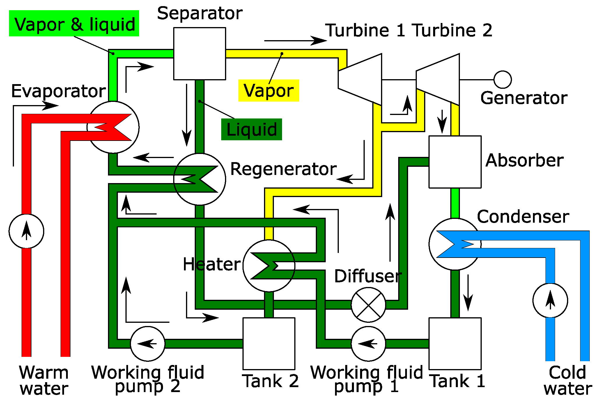
Figure 1. Overview of OTEC plant using Uehara cycle.
Jmse 06 00018 g001
Figure 2. Warm source side model and cold source side model.
Jmse 06 00018 g002
Figure 3. Experimental data of working fluid flow rate m ˙ L I P M 1 as input. (a) m ˙ L I P M 1 = 1.67 kg / s (Min.: 1.542 kg / s , Max.: 1.675 kg / s ); (b) m ˙ L I P M 1 = 1.94 kg / s (Min.: 1.878 kg / s , Max.: 1.994 kg / s ); (c) m ˙ L I P M 1 = 2.22 kg / s (Min.: 2.189 kg / s , Max.: 2.300 kg / s ); (d) m ˙ L I P M 1 = 2.50 kg / s (Min.: 2.433 kg / s , Max.: 2.536 kg / s ); (e) m ˙ L I P M 1 = 2.78 kg / s (Min.: 2.711 kg / s , Max.: 2.839 kg / s ); (f) m ˙ L I P M 1 = 3.33 kg / s (Min.: 3.242 kg / s , Max.: 3.350 kg / s ).
Jmse 06 00018 g003
Figure 4. Experimental data of power generation G exp T B ( t ) as output. (a) m ˙ L I P M 1 = 1.67 kg / s (Min.: 17.10 kW , Max.: 17.35 kW ); (b) m ˙ L I P M 1 = 1.94 kg / s (Min.: 29.65 kW , Max.: 30.10 kW ); (c) m ˙ L I P M 1 = 2.22 kg / s (Min.: 40.55 kW , Max.: 41.10 kW ); (d) m ˙ L I P M 1 = 2.50 kg / s (Min.: 42.80 kW , Max.: 43.75 kW ); (e) m ˙ L I P M 1 = 2.78 kg / s (Min.: 46.05 kW , Max.: 46.55 kW ); (f) m ˙ L I P M 1 = 3.33 kg / s (Min.: 44.20 kW , Max.: 46.25 kW ).
Jmse 06 00018 g004
Figure 5. Constructed models. (a) Warm source side models; (b) Cold source side models.
Jmse 06 00018 g005
Figure 6. Input m ˙ L I P M 1 ( t ) for simulation based on experimental results (Min.: 1.542 kg / s , Max.: 3.350 kg / s ).
Jmse 06 00018 g006
Figure 7. Output G exp T B ( t ) for simulation based on experimental results (Min.: 17.15 kW , Max.: 46.55 kW ).
Jmse 06 00018 g007
Figure 8. Simularion results of G T B ( t ) by warm source side model. (a) Results by constructed model from data (1) (Min.: 16.75 kW , Max.: 47.13 kW ); (b) Results by constructed model from data (2) (Min.: 14.22 kW , Max.: 45.95 kW ); (c) Results by constructed model from data (3) (Min.: 11.73 kW , Max.: 47.46 kW ).
Jmse 06 00018 g008
Figure 9. Simularion results of G T B ( t ) by cold source side model. (a) Results by constructed model from data (1) (Min.: 18.23 kW , Max.: 45.87 kW ); (b) Results by constructed model from data (2) (Min.: 16.00 kW , Max.: 44.91 kW ); (c) Results by constructed model from data (3) (Min.: 13.04 kW , Max.: 45.61 kW ).
Jmse 06 00018 g009
Table 1. Experimental condition.
Parameter (Unit)Value
Temperature of Warm Water ( C)30
Temperature of cold water ( C)9
Flow rate of warm water (kg/s)111.1
Flow rate of cold water (kg/s)111.1
Mass fraction of working fluid (kg/kg)0.97
Flow rate of working fluid (kg/s)1.67, 1.94, 2.22, 2.50, 2.78, 3.33
Sampling time (s)10
Table 2. Orders of polynomials of constructed models.
(a) Warm Source Side Model
Data(1)(2)(3)
Polynomial f W 1 311
Polynomial f W 2 422
Polynomial f W 3 411
Polynomial f W 4 323
Polynomial f W 5 311
Polynomial f W 6 112
Polynomial f W 7 313
IAE (kW·s)1254.01207.42025.2
(b) Cold Source Side Model
Data(1)(2)(3)
Polynomial f C 1 134
Polynomial f C 2 214
Polynomial f C 3 231
Polynomial f C 4 123
Polynomial f C 5 432
Polynomial f C 6 222
IAE (kW·s)1600.72222.82851.2
Table 3. IAE by warm source side model.
(a) IAE by Warm Source Side Model Constructed from Data Interval (1)
Working Fluid Flow Rate
m ˙ LI PM 1 (kg/s)
1.671.942.222.502.783.33Total
Input (a) (kW·s)59.9159.7169.1681.5109.8275.11455.1
Input (b) (kW·s)126.8115.9213.7628.9119.3174.91379.6
Input (c) (kW·s)84.8147.5237.2649.7110.6167.01396.7
(b) IAE by Warm Source Side Model Constructed from Data Interval (2)
Working Fluid Flow Rate
m ˙ LI PM 1 (kg/s)
1.671.942.222.502.783.33Total
Input (a) (kW·s)114.7104.6630.342.6102.5275.91270.6
Input (b) (kW·s)197.1125.9666.3122.8107.0322.91542.0
Input (c) (kW·s)174.493.8687.995.894.2301.81447.9
(c) IAE by Warm Source Side Model Constructed from Data Interval (3)
Working Fluid Flow Rate
m ˙ LI PM 1 (kg/s)
1.671.942.222.502.783.33Total
Input (a) (kW·s)772.9244.0210.9227.7270.1284.42010.0
Input (b) (kW·s)840.7250.0182.4207.8268.4306.42055.6
Input (c) (kW·s)764.2224.0162.3220.7262.7232.81866.7
Table 4. IAE by cold source side model.
(a) IAE by Cold Source Side Model Constructed from Data Interval (1)
Working Fluid Flow Rate
m ˙ LI PM 1 (kg/s)
1.671.942.222.502.783.33Total
Input (a) (kW·s)275.6166.681.4469.4169.6750.41913.0
Input (b) (kW·s)301.2224.560.8442.8158.81419.92607.9
Input (c) (kW·s)275.1158.268.1457.7169.4762.01890.5
(b) IAE by Cold Source Side Model Constructed from Data Interval (2)
Working Fluid Flow Rate
m ˙ LI PM 1 (kg/s)
1.671.942.222.502.783.33Total
Input (a) (kW·s)73.0610.2836.826.0429.31125.43100.7
Input (b) (kW·s)66.7479.6835.035.1427.92040.33884.6
Input (c) (kW·s)85.2548.1819.937.1423.81158.03072.1
(c) IAE by Cold Source Side Model Constructed from Data Interval (3)
Working Fluid Flow Rate
m ˙ LI PM 1 (kg/s)
1.671.942.222.502.783.33Total
Input (a) (kW·s)803.2362.2941.5423.2161.5196.82888.3
Input (b) (kW·s)805.6436.2928.4434.1158.7243.43006.4
Input (c) (kW·s)786.9324.4911.2440.2154.8225.52843.1
Table 5. Average of calculation time.
(a) Warm Source Side Model
Data(1)(2)(3)Average (s)
Input (a)0.023670.023200.023610.02349
Input (b)0.023340.023240.023130.02324
Input (c)0.023370.023210.022990.02319
Average (s)0.023460.023220.023240.02331
(b) Cold Source Side Model
Data(1)(2)(3)Average (s)
Input (a)0.019440.019290.019480.01940
Input (b)0.019360.019870.019320.01951
Input (c)0.019260.019400.019490.01938
Average (s)0.019350.019520.019430.01943