1. Introduction
The growing global shipping rates are generating increasing acoustic output in the underwater environment. The deep-ocean noise levels have grown over the past four decades, correlating with the observed increase in global shipping rates [
1]. In addition, the adverse effects of shipping noise on marine mammals raised concern in the 1970s when the overlap between the main frequencies used by large baleen whales and the dominant components of noise from ships was noted [
2]. Fish have also been observed to be disturbed by noise emitted from ships [
3]. The sound emitted from naval and research vessels and submarines can interfere with measurement equipment, or can be used for detection. The noise emitting into the interior of the ship may disturb the crew as well as the passengers on board and increase hull vibration levels. The noise emission levels are especially important for cruise liners and yachts from the points of view of comfort and the mission of the ship.
Marine propellers are an important source of noise emitted from ships to the underwater environment and to the interior of the vessel. A non-cavitating propeller induces discrete peaks to the noise spectrum, which occur at the blade passing frequency and its multiples. These peaks are related to blade thickness and loading-induced pressure pulses. In addition, a propeller induces broadband noise, which is related to unsteadiness in the flow field. This corresponds to the turbulent fluctuations in the velocity and pressure fields. In the case of phase changes, the underwater noise from cavitation usually dominates other propeller-induced noise (excluding singing), and all other underwater noise from a ship [
4]. Sheet and tip vortex cavitation generally increase the amplitude of the tonal pressure fluctuations, and cavitating vortices can also act as a source of broadband excitation [
5,
6,
7]. Additionally, unsteady cavitation structures such as cloud and bubble cavities give rise to the propeller-induced broadband signature.
During the past decade, CFD (computational fluid dynamics) has been actively utilized to study propeller performance in wetted and cavitating conditions [
8,
9,
10,
11,
12,
13,
14,
15,
16,
17,
18,
19,
20]. For instance, Turunen et al. [
9], Asnaghi et al. [
21], and Lidtke et al. [
22] have investigated single- and two-phase propeller flows using the open-source CFD toolbox OpenFOAM. Flow structures in the wake and tip vortex of a propeller employing different RANS (Reynolds-averaged Navier–Stokes) or scale-resolving turbulence closures have been studied by Sipilä et al. [
23], Guilmineau et al. [
24], and Viitanen and Siikonen [
25]. Additionally, higher-fidelity turbulence closures such as the LES or DES (large eddy simulation or detached eddy simulation, respectively) approaches have been used to compute the flow past marine propellers by Liefvendahl et al. [
26], Lu et al. [
10], Muscari et al. [
11], Ji et al. [
27], Chase and Carrica [
28], and Balaras et al. [
12]. For example, Ji et al. [
27] simulated a cavitating marine propeller using a partially averaged Navier–Stokes (PANS) modelling approach, whereas Chase and Carrica [
28] studied a submarine propeller with several turbulence modelling approaches including a coarse direct numerical simulation (DNS) method. Moreover, Balaras et al. [
12] conducted investigations using LES in conjunction with an immersed boundary method. Specific attention towards the peculiar nuisance of propeller-induced noise has been given, for example, by Ianniello et al. [
29], Lloyd et al. [
30], and Lidtke et al. [
22] via utilization of the Ffowcs Williams–Hawkings acoustic analogy, where the CFD results of the propeller flow dynamics were utilized as source terms for the acoustic simulations. Budich et al. [
31] studied the Potsdam propeller test case (PPTC) in cavitating conditions, focusing on the shock wave dynamics and including an erosion assessment with a compressible flow solver.
The most general approach for acoustic simulations concerns the DNS, since the flow solution then includes both sound generation and its propagation. Unfortunately, DNS is computationally very expensive and limited to problems with low Reynolds numbers. Acoustic analogies may be utilized for the assessment of flow-induced noise based on an a priori flow solution, and the noise propagation is evaluated from the results of the flow simulation. Several different acoustic analogies are reviewed by Uosukainen [
32]. Computationally-less-intensive integral methods can be used for external problems, but for practical cases (e.g., propeller in a cavitation tunnel), the assumption of a free-field space may not be valid. Then, one option is to use the variational formulation of Lighthill’s analogy in the finite element method (FEM) context. We have chosen the latter approach for the investigations presented here. With this procedure, moving boundaries are naturally taken into account, and there are no limitations on the elasticity or geometry of the surrounding boundaries [
33]. In the present acoustic solution, the different types of sound sources are not explicitly distinguished, and we do not utilize the pressure provided by the flow solution. Instead, the acoustic sources are evaluated from the so-called Lighthill tensor, which comprises the flow momentum components. On the other hand, our approach requires a volumetric discretization of the acoustic domain.
In this paper, we study a model-scale propeller, specifically the PPTC, in a uniform homogeneous inflow condition. We conducted wetted and cavitating DDES (delayed DES) of the propeller to investigate the influence of not only global blade loading effects but also transient wake characteristics and turbulent vortical flow structures, as well as sheet and tip vortex cavitation, on the harmonic and broadband noise. The combined hydrodynamic–hydroacoustic problem was solved via a hybrid approach. In the hybrid method, we assume that the flow solution based on DDES is decoupled from the acoustic propagation, which is composed of an acoustic FEM computation. The effective assumption is that the acoustic field does not modify the bulk flow solution. Consequently, we solve the flow problem independently of and prior to the solution of the acoustic problem.
We conducted the flow simulations with the general-purpose CFD solver
Finflo [
8,
34]. The code has been applied to both cavitating and non-cavitating propeller flows [
23,
25,
35]. The propeller-induced sound pressure levels were obtained using
Actran [
33]. We concentrated on one propeller operation point in wetted and cavitating conditions for the hydroacoustic analyses. Similar hybrid CFD–CHA (computational hydroacoustics) investigations were carried out for the PPTC propeller by Hynninen et al. [
36] and Viitanen et al. [
37].
In the next section, the hydrodynamic and hydroacoustic modelling approaches are described. Then, the test case is introduced, followed by an assessment and validation of the numerical results. Finally, conclusions are drawn from the presented results.
2. Flow Solution
2.1. Governing Equations
The flow model applied is based on a homogeneous flow assumption, which is a common assumption as far as cavitation is concerned [
38]. The governing equations for the cavitation model are
where
p is the pressure,
the absolute velocity in a global non-rotating coordinate system, and
the stress tensor,
is a void (volume) fraction of phase
k,
the density,
t the time,
the mass-transfer term, and
the gravity vector. The void fraction is defined as
, where
denotes the volume occupied by phase
k of the total volume,
. For the mass transfer
holds, and consequently only a single mass-transfer term is needed.
Although the phase temperatures do not play a significant role in cavitation, the energy equations are always solved in the present method. The aim is to apply a compressible form of the equations. In order to predict the correct acoustic signal speeds, a complete model is needed. The phase temperatures
and
also have some influence on the solution via the material properties that are calculated as functions of the pressure and phase temperatures. The calculation of the material properties is described in [
39]. The sound speed
c for a two-phase mixture is defined as
In the expressions above, the indices g and l refer to gas and liquid phases, respectively, and denotes the enthalpy of phase k.
The energy equations for phase
g or
l are written as
Here
is the specific internal energy,
the heat flux,
interfacial heat transfer from the interface to phase
k, and
saturation enthalpy. Since
, by adding the energy equations together, the following relationship is obtained between the interfacial heat and mass transfer
Above,
is a heat transfer coefficient between the phase
k and the interface. The interfacial heat transfer coefficients are based on the mass transfer, as shown in
Section 2.5.
The momentum and total continuity equations in the homogeneous model do not change, except for the material properties like density and viscosity, which are calculated as
where
is the dynamic viscosity. The turbulence effects are currently handled using single-phase models for the mixture.
2.2. Finite-Volume Form
Equation (
1) can be written in a general finite-volume form for a cell
as
where the sum is taken over all cell surfaces
j,
is a surface normal on a cell face, and
the cell face area. The mass flux
can be identified in all field equations. In Equation (6), a Rhie–Chow-type damping term is added via the convective velocity
. Instead of the commonly used scaling, the term is scaled using an artificial sound speed [
40]. Pressure differences are applied and the flux terms are written in terms of the void fraction. However, the implicit solution is based on mass fractions:
This form in the implicit stage is convenient, since the same mass flows can be used in the Jacobian matrices as in the case of the momentum equation.
Equation (6) can be applied for arbitrary cell shapes, although in the present solution a structured grid is applied. For the time derivatives, a second-order three-level fully implicit method is used. The viscous fluxes as well as the pressure terms are centrally differenced. For the convective part, the variables on the cell surfaces are evaluated using a third-order upwind-biased MUSCL (monotonic upstream-centred scheme for conservation laws) interpolation [
41]. A flux limiter can be applied, but in this study this is done only for the void fraction. The application of a limiter function to the convective fluxes of the void fraction may be necessary, since it is essentially a discontinuous quantity through the phase boundary. This may lead to problems in a numerical solution, and the void fraction could locally obtain non-physical values amidst an iterative solver. Additionally, cavitation volumes can exhibit rapid temporal and spatial variation when, for instance, bursts of cloud cavities or fine cavitating vortices are present. Previously, it was shown that a compressive limiter with the void fraction equation especially improves the predicted tip vortex cavitation patterns [
25]. Hence, a compressive “superbee” limiter of Roe [
42] is employed for the cavitating cases considered in this study as well. A review of the high-resolution limiters for two-phase flows is given, for example, in [
43].
2.3. Solution Algorithm
The solution method is a segregated pressure-based algorithm where the momentum equations are solved first, and then a pressure–velocity correction is made. The basic idea in the solution of all equations is that the mass balance is not forced at every iteration cycle, but rather the effect of the mass error is subtracted from the linearized conservation equations. A pressure correction equation was derived from the continuity Equation (
1) linked with the linearized momentum equation. The method is based on the corresponding algorithm for a single-phase flow [
40], and is described in detail in Ref. [
25]. The resulting pressure-correction equation is
where
is the pressure change in the cell on the other side of face
j,
the diagonal term of the Jacobian matrix of the linearized momentum equation, and
an error in mass balance for phase
k. The first term on the left-hand side is a result of the compressibility, but mainly serves as an under-relaxation for the pressure. An extra multiplier of 0.01 was added on the basis of test calculations. Another parameter
is used to control the pressure changes caused by the mass-transfer term [
25].
Two different solution strategies were utilized for the simulations of the flow around the rotating propeller. The first one was to rotate the computational domain with the propeller rate of revolution, and integrate the governing equations in the physical time. Consequently, results obtained from this strategy are referred to as transient. The second approach exploited the fact that the governing equations can yield a steady-state solution when the equations are expressed in the coordinate system that is rotating with the propeller. This solution method is then referred to as quasi-steady.
In the transient simulations, a steady-state solution was sought within each physical time-step by iterating until the norms of the main variables decreased by a sufficient amount (i.e., at least 2–3 orders of magnitude). Approximately 100 inner iterations were usually required within each physical time-step for non-cavitating simulations. In the present study, between 150–200 inner iterations were made for the cavitating simulations.
In the quasi-steady approach, absolute velocities were used in the solution, and the rotational movement of the propeller was accounted for in the convection velocity and as source terms in the y- and z-momentum equations as the propeller was rotating around the x-axis. The equations were iterated until the global force coefficients and the norms of the main variables obtained a sufficiently steady level, with the norms having decreased to .
2.4. Turbulence Modelling
Nominally a Reynolds-averaged form of Equations (
1)–(
3) was used, and the delayed detached-eddy simulation (DDES) [
44] that combines RANS and LES was also applied in the same form. Usually, in cavitation modelling, turbulence is taken into account using single-phase closures. Also in this study, the turbulence modelling was applied for the homogeneous mixture. The choice of turbulence closure plays an essential role in the numerical prediction of the performance of a marine propeller. While the global forces or steady cavitation patterns near the blades generally might not considerably differ between the turbulence closures, the utilized model can have a significant influence on unsteady flow structures, or on the flow in the wake of the propeller. In the case of unsteady propeller cavitation, capturing the cavitation dynamics is crucial in order to assess not only the performance but also the erosive tendency of collapsing cavities, as well as the induced underwater noise. Moreover, accurate prediction of the wake flow is important when considering the propeller–rudder, propeller–pod, or multi-propeller interactions.
In this study, DDES is based on the shear stress transport (SST)
-model [
45]. DDES is a slightly modified version of the detached-eddy simulation (DES). DES and DDES reduce to a RANS model in regions where the largest turbulent fluctuations are of a smaller size than the local grid spacing. Both are hybrid RANS/LES models, and function as an LES subgrid-scale model in regions where the local turbulent phenomena are of greater size than the local grid spacing [
46]. A time-accurate solution is made to resolve turbulent fluctuations. In the present study, the calculations were performed up to the wall, and the height of the first cell was adjusted such that the non-dimensional wall distance
for the first cell, with
being the friction velocity,
the wall shear stress, and
d is the normal distance from the solid surface to the centre point of the cell next to the surface.
In DES, the equation for the turbulent kinetic energy (
k) can be written with a modified dissipation term as [
47]:
where
P is the production of turbulence,
is the length scale, and
D is the diffusion term. The DES length scale was computed as the minimum of the RANS length scale,
, and the local resolution
. Here
was a model constant. The parameter
was evaluated as the minimum of the local wall distance, and the grid resolution
, where
denotes the thickness of the cell in different index directions. The DES length scale was then
and the coefficient
was computed from
where the constants were
,
, and
is Menter’s blending function [
45]. Furthermore, when utilizing DDES, the length scale is replaced by the expression [
44]
Here
outside the boundary layer, and the length scale becomes
if the grid spacing permits. The DDES variant of DES aims to improve the accuracy compared to Equation (10), which has in some instances been observed to cause grid-induced separation.
2.5. Mass and Energy Transfer
A number of mass-transfer models have been suggested for cavitation [
48]. Usually, the mass-transfer rate is proportional to a pressure difference from a saturated state or to a square root of that. In this study, the mass-transfer model is similar to that of Choi and Merkle [
38]:
where
is the saturation pressure,
the reference (inlet) density, and
the corresponding velocity. The evaporation time constants were made non-dimensional using the reference length
and the velocity related to cavitation (
). In some cases, such as on a propeller blade, the cavitation length and velocity differ from the reference length
and the reference velocity (
). The time constants correspond to the parameters of the original model as
and
. The empirical parameters of the cavitation model are calibrated in [
49].
In the present method, the saturation pressure was based on the free-stream temperature, and the gas phase was assumed to be saturated (i.e.,
). Liquid temperature varies less because of the mass and energy transfer. Since the gas temperature was forced to be
,
. From Equation (4), the interfacial heat transfer can be solved for the liquid phase
Using Equations (13) and (14), the interfacial transfer terms in the continuity and energy equations can be solved.
In order to decrease the oscillations in the solution owing to the rapid changes in the mass transfer, the mass-transfer rate was under-relaxed between the iteration cycles as , where is an under-relaxation factor, n refers to the iteration cycle, and is calculated from Equation (13). For small values , under-relaxation was not applied. The under-relaxation factor and the limit are quite arbitrary, although tested by numerous simulations.
3. Acoustic Solution
Instead of the direct solution of the compressible Navier–Stokes (N-S) equations, the hydrodynamic and hydroacoustic problems are treated separately. The former is obtained from compressible N-S equations (Equations (
1)–(
3)) using DDES, while the latter can be seen as a subsequent solution of the compressible N-S equations in isentropic conditions. The acoustic problem is analogous to a direct solution in the sense that the flow-generated noise propagates not through the mean flow, but according to a wave operator in a medium at rest. In this analogous problem, source terms are utilized to represent the flow. The effectively two-step approach requires one unsteady flow solution in the time domain and one subsequent acoustic analysis in the frequency domain.
The present solution to the acoustic problem is based on the acoustic analogy using the
Actran code [
33]. The propagation problem, in which noise is generated by flow fluctuations, is replaced by an analogous problem, where the propagation is represented by a wave operator. In this study, the analogy of Lighthill [
50] is used, which utilizes a wave equation for density. The wave equation can be derived by taking the time-derivative of the continuity equation, and the gradient of the momentum equations. Combining these two yields
where
is the speed of sound in the medium, and
the Lighthill tensor. Furthermore,
can be simplified by assuming isentropic, high-
, and low-
flows to comprise only the fluid momentum components, or
. The wave equation can be transformed to the frequency domain
where
is the angular frequency. In
Actran, the solution of the acoustic problem, Equation (15), is based on variational formulation of the wave equation for density propagation, transformed into the frequency domain, Equation (16). The code requires the Lighthill tensor in the frequency domain as an input. The source terms
are related solely to the momentum components, which are provided by the flow solution.
In
ACTRAN, instead of the density a transformed potential,
, defined through
is used. The alternative equation for the Lighthill analogy is then
The weak variational formulation for the density propagation in the frequency domain involving stationary and moving geometry reads
where
is the volume and
is the surface of the boundary enclosing the propeller. Using this formulation, the volume and surface source term influences can be evaluated. The quadrupole sources (e.g., due to turbulence) are included in the volume term, whereas the monopole and dipole sources are taken into account in the surface source term.
Two types of source terms are present in Equation (19). The surface source terms are evaluated on the surface surrounding the propeller blades and hub. Conformal surface enclosing the propeller is shown in
Figure 1. The noise generation resulting from flow phenomena such as turbulence, blade loading, and cavitation take place inside the volume surrounding the blades and the hub, as shown in
Figure 1, which is accounted for by mapping the sources as defined in Equation (19) onto the enclosing surface. In practice, in order to achieve the most accurate source description, the surface should be located close to the source (i.e., the unsteady flow). The volume mesh encloses the propeller and the wake region as shown in
Figure 1, and the volume source terms in Equation (19) are evaluated in these volume elements. The hydroacoustic source terms are calculated in the time domain using oversampling by default at every half CFD time step to avoid aliasing effects during the Fourier transform, and are saved in an NFF database. The calculated hydroacoustic source terms are then transformed on the acoustic mesh by integrating over the CFD mesh using the shape functions of the acoustic mesh.
4. Computational Case
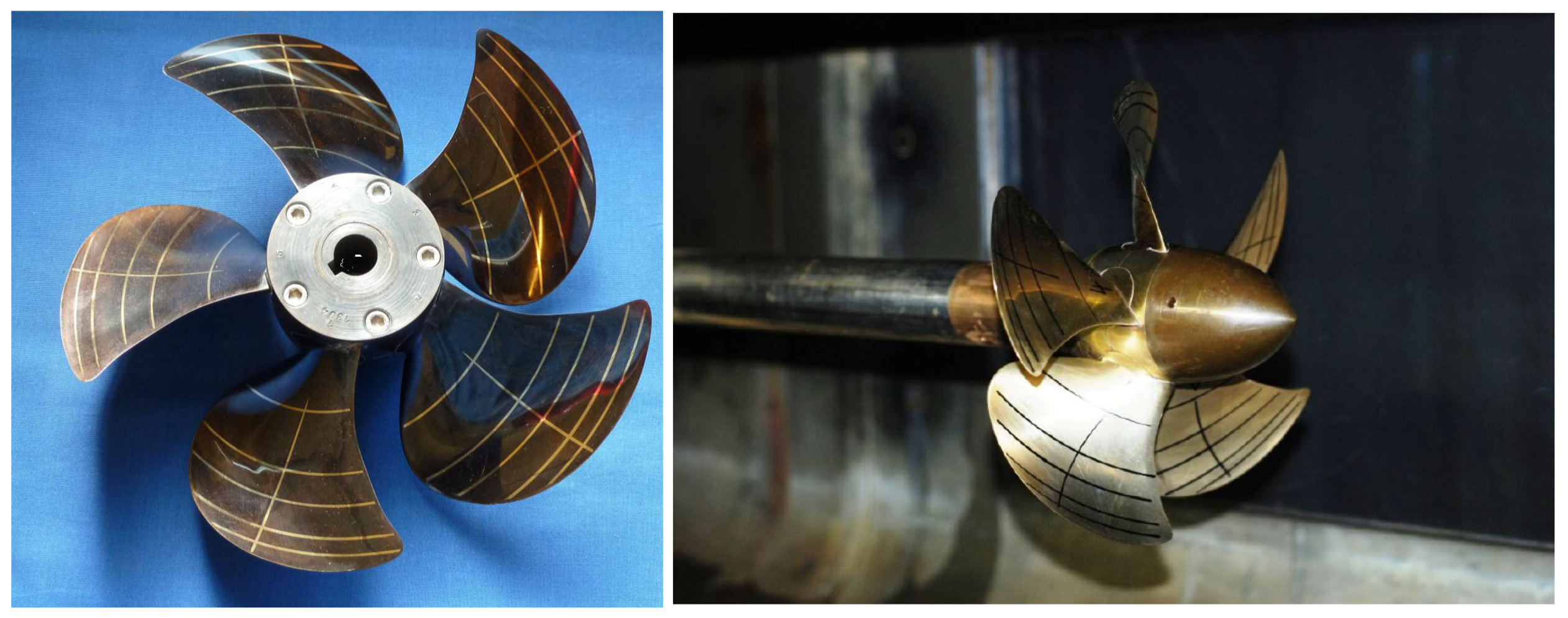
The computational case was the PPTC propeller [
51]. The diameter of the model-size propeller is 0.250 m. The propeller has five blades, and a right-handed direction of rotation. The skew of the propeller is moderate.
Table 1 summarizes the main geometrical parameters of the PPTC propeller. Photographs of the propeller are shown in
Figure 2. A large database of experimental results has been made available by SVA Potsdam (
http://www.sva-potsdam.de/pptc-smp11-workshop/).
We investigated the propeller operating in push configuration (i.e., the shaft was located in front of the propeller), and we considered three propeller points of operation. One operating point was simulated both in wetted and cavitating conditions, while the other two cases were simulated only in wetted conditions. The simulations were performed using a constant rate of revolution,
. The advance coefficient and the cavitation number are defined as
respectively, where
is the propeller speed of advance,
n is the propeller rate of revolution,
D is the propeller diameter,
p is the pressure,
is the saturation pressure, and
the fluid density. The first investigated operation point was
in wetted conditions as well as in cavitating conditions with
. The second non-cavitating case had the advance coefficient
, and the third non-cavitating operating point was
. The first propeller operating point corresponds to the PPTC Case 2.3.1 of smp’11 Workshop [
52], while the cavitation tunnel LDV (laser Doppler velocimetry) measurements of the propeller were carried out for the second operating point [
53]. The third operating point corresponds to Case 2.3.3 of the smp’11 Workshop. The thrust and torque of the propeller were non-dimensionalized as
respectively, where
T denotes the thrust and
Q the torque of the propeller. Finally, the open water efficiency of the propeller is defined as
Below, we describe first the CFD numerical setup utilized, the grid, and related boundary conditions, followed by a corresponding description of the numerical setup used in the hydroacoustic simulations.
4.1. CFD: Numerical Setup, Grid, and Boundary Conditions
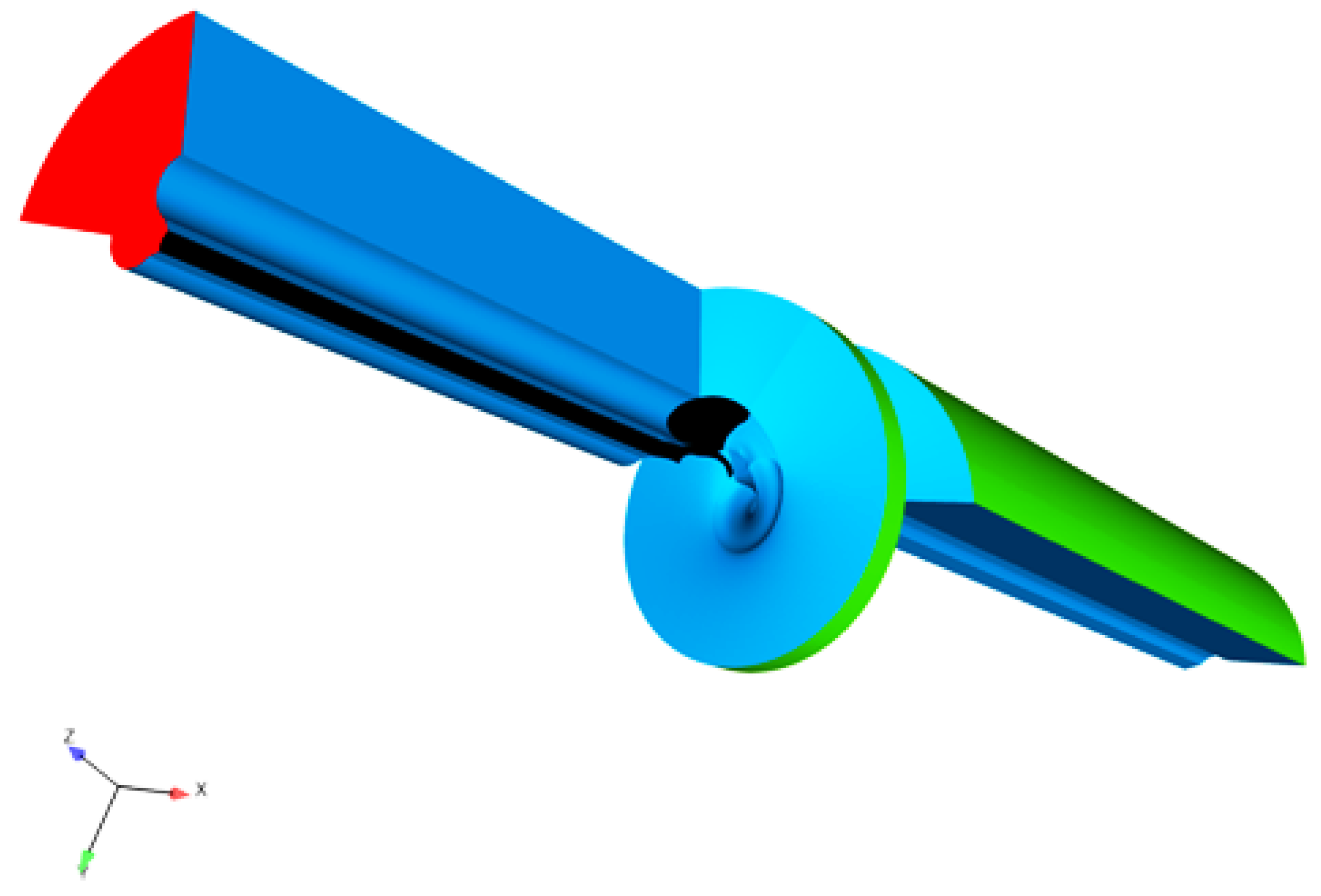
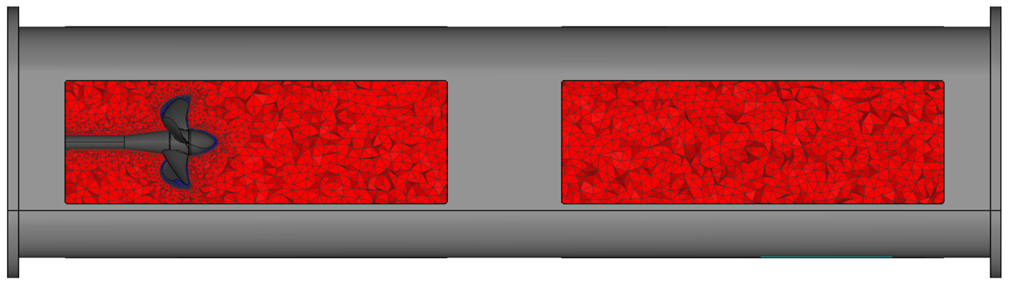
The structured computational grid used consists of roughly 5.5 million cells in 28 grid blocks. The computational domain is shown in
Figure 3. Due to the symmetric nature of the problem of a propeller operating in axial uniform inflow, only one blade was modelled. The blades, hub, and shaft were modelled as no-slip rotational surfaces, coloured black in
Figure 3. Boundary-layer transition to turbulent flow was not taken into account in the present simulations. A velocity boundary condition was applied at the inlet, denoted as the red face, and a pressure boundary condition was applied at the outlet. A slip boundary condition was applied at the simplified tunnel walls, which are coloured green in
Figure 3. Cyclic boundaries are denoted by the blue faces, and the whole computational domain was considered as rotating with the given rate of rotation. The inflow velocity was set based on the advance numbers of the propeller, and the background pressure level was set based on the cavitation number. The inlet was located five propeller diameters upstream of the propeller, and the outlet was located ten diameters downstream of the propeller. The rectangular cavitation tunnel of SVA Potsdam was here modelled as a circular duct of the same cross-sectional area, thus enabling also the quasi-steady computation of the problem. The radius of the computational domain was then 0.3385 m.
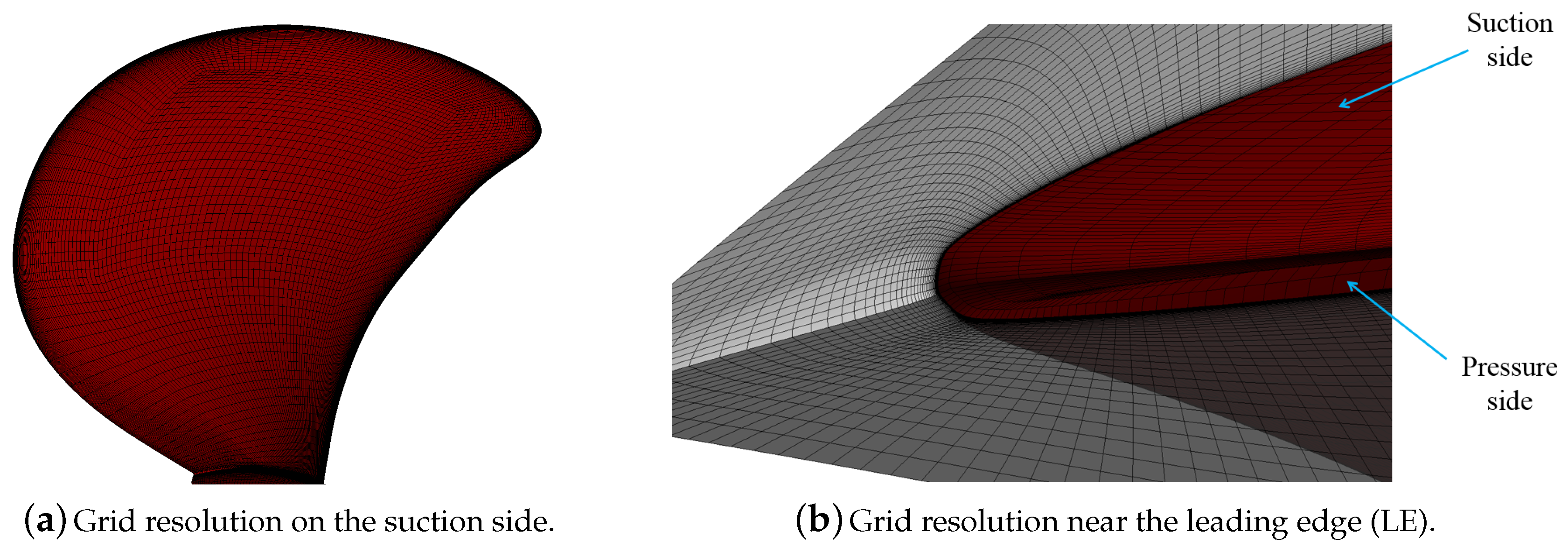
The surface grid on the suction side of the blade is shown in
Figure 4a. The surface grid on the pressure side of the blade was similar. The grid had an O-O topology around the propeller blades. The grid resolution around the leading edge was fine, as shown in
Figure 4b, and there were about 30 cells around the leading-edge radius. Due to the O-O topology, the same resolution was applied around the blade tip and the trailing edge as well. The grid was refined normal to the viscous surfaces such that
.
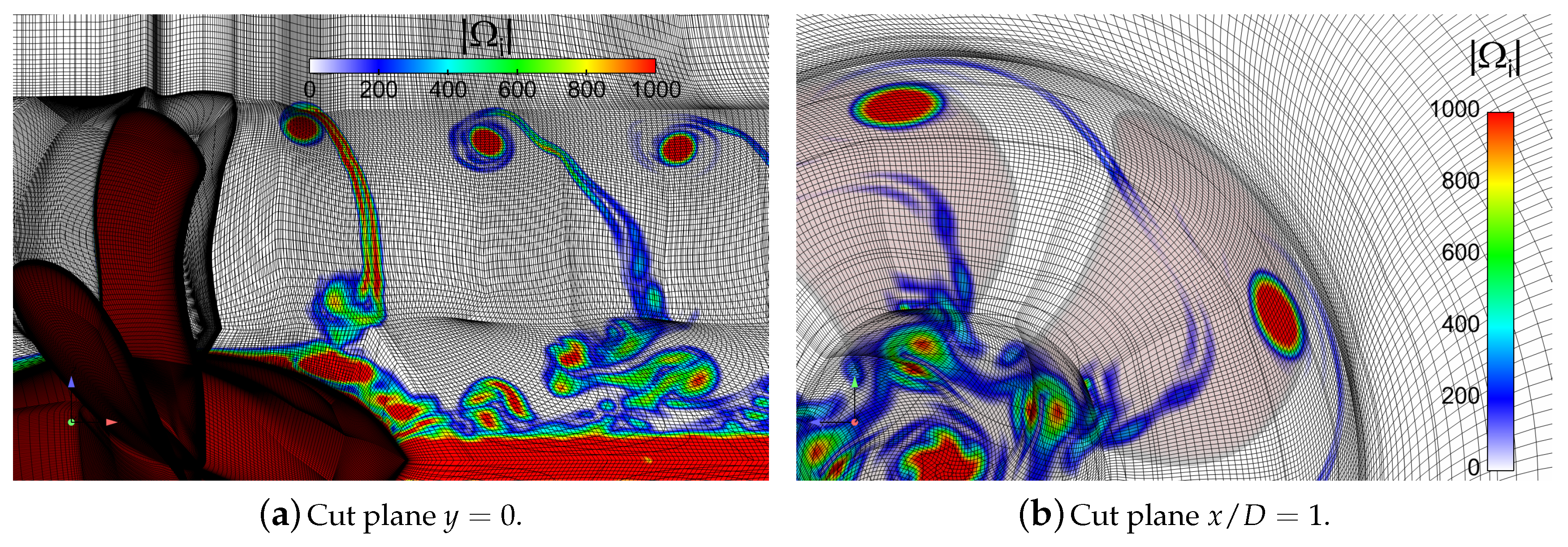
The grid points in the helical blocks located downstream of the propeller were adaptively concentrated in the region of the tip vortex, based on the propeller loading.
Figure 5 depicts the concentration of the grid points near the tip vortex induced by the rotating blades. In the figure,
denotes the absolute value of vorticity, and the propeller blades, hub, and shaft are coloured dark red. The figure shows exemplary views of the resolution on the finest grid, demonstrating that the tip vortex was well-maintained even beyond
. There were roughly
grid points in the cross-section of the tip vortex on the finest grid on the plane
. The helical blocks in the slipstream of the propeller were extended to a pitch corresponding to approximately
of rotation from the propeller plane.
The calculations were performed on three grid levels. On a coarse grid level, every second point in all directions was removed compared to a finer level grid. The fine grid had roughly 5.5 million cells, the medium grid roughly 0.7 million cells, and the coarse grid approximatively 0.08 million cells. The computations were initiated such that a quasi-steady solution was first obtained on the coarse grid, which was then used as an initial guess for the medium grid quasi-steady simulations. After a quasi-steady solution was obtained on the medium grid, time-accurate simulation was continued on the medium grid from the quasi-steady results for approximately 10 propeller revolutions. The quasi-steady solutions were obtained using Chien’s low-Reynolds-number
turbulence model [
54], and all transient approaches relied on DDES. The results of the time-accurate medium grid simulations were then used as an initial guess for the time-accurate simulations on the fine grid, and usually 5–10 propeller revolutions (or 25–50 propeller blade passages) were simulated on the fine grid. The presented approach is a relatively fast and overall efficient computational procedure for single and two-phase DDES of marine propellers. In the time-accurate simulations, a physical time-step of
s was used, which corresponds to half a degree of propeller rotation. In this paper, we present the results that were obtained on the fine grid from time-accurate simulations.
4.2. CHA: Numerical Setup, Grid, and Boundary Conditions
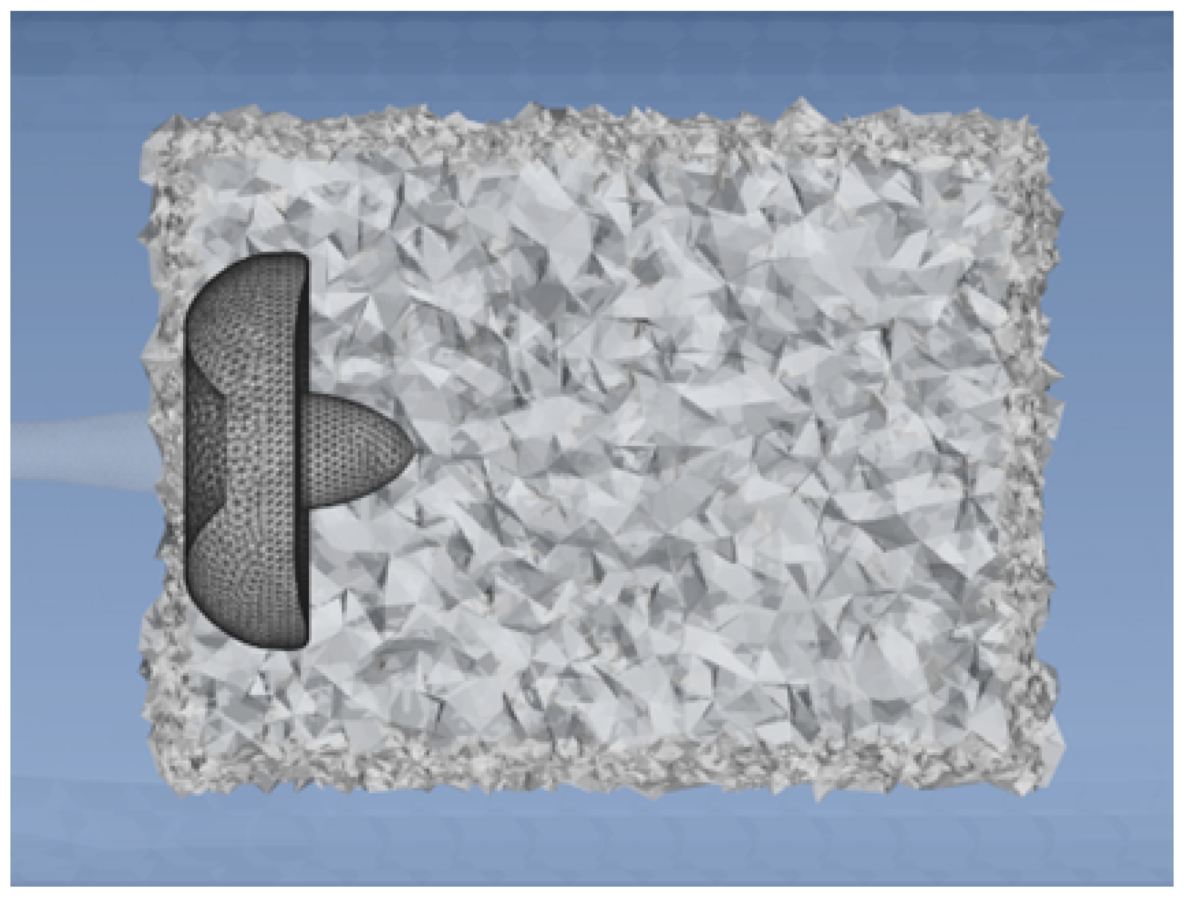
The acoustic FE mesh is shown in
Figure 6, where the propeller is modelled inside the cavitation tunnel. There were more than six elements for the shortest wave length. In total, there were 450,000 quadratic tetrahedron elements in the mesh. At both ends of the cavitation tunnel, non-reflecting boundary conditions were used. The tunnel walls were modelled as rigid. The maximum frequency that can be resolved within the acoustic analyses is limited by the Nyqvist frequency and the time step used in the transient CFD computations, or
. In the CFD simulations, every second time-step was written for the acoustic simulation (i.e., with a time-step corresponding to one degree of propeller rotation). The lowest frequency that could be resolved,
, was set by the physical simulation time chosen for the CFD–CHA coupling, which in this case was one propeller revolution. While the transient CFD simulations were conducted for up to ten propeller revolutions, the flow solution of the final propeller revolution was used as input for the CHA simulations.
5. Results
Next, we report the results of DDES for the wetted and cavitating cases, followed by the CHA results. First, the global forces (i.e., the thrust, torque, and open water efficiency of the propeller) are given, followed by an assessment of flow and cavitation patterns near the propeller and in its wake. Finally, we show the results of the CHA simulations. In all figures depicting the propeller, unless stated otherwise, a snapshot of the simulations with the blade at the top dead centre position is shown, depicting instantaneous flow structures near the propeller. We compare the simulated and experimentally-determined propeller global performance characteristics at all studied advance numbers. The propeller wake was validated at , whereas we carried out detailed investigations of the wake flow structures and acoustic excitation at both in wetted and cavitating conditions.
5.1. Validation and Cavitation Observations
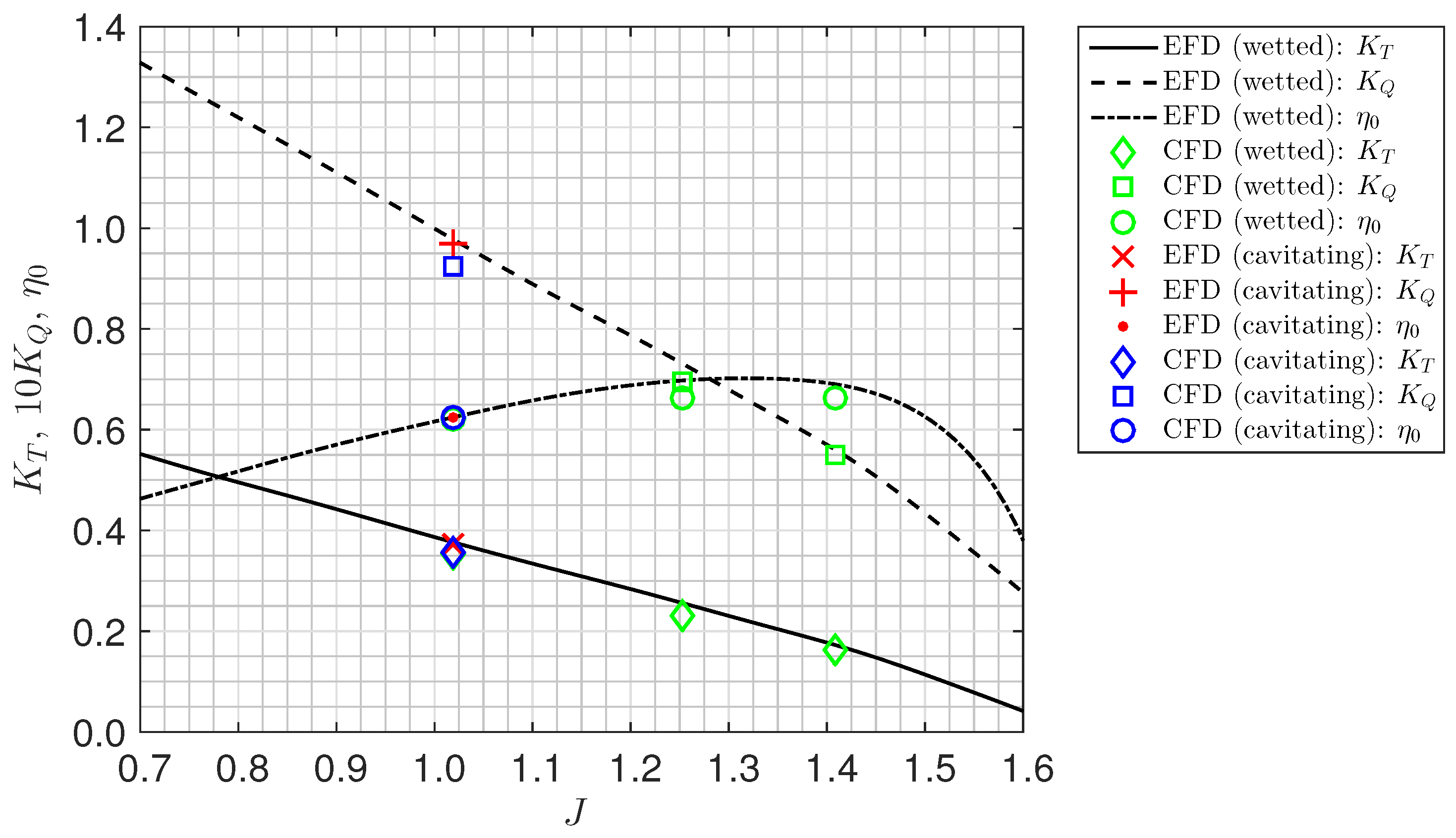
A comparison of propeller performance characteristics is shown in
Figure 7 in both wetted and cavitating conditions. The experimental results are given by Barkmann [
55] for the wetted conditions, and by Heinke [
51] for the cavitating conditions. In the figure, the CFD results are given for the wetted and cavitating cases at
, and for the wetted cases at
and
. Corresponding experimental results for the cavitating condition are shown as markers. The CFD-predicted open water characteristics were in good agreement with the experimental data, although the simulations tended to under-predict the thrust and torque of the propeller. For the lowest investigated propeller loading condition, the simulations agreed better with the experiments than for the two higher loadings. Overall, the thrust coefficient differed from the experimental results by 2–8% in the wetted case, whereas the difference was smaller for the investigated cavitating case, 3%. The torque coefficient agreed better with the experiments, and the differences were within 1–3% for both the wetted and cavitating cases. Deviations in the EFD (experimental fluid dynamics) and CFD propeller global forces could be due to various reasons, other than limitations in the numerical method. Possible confinement effects due to the geometry of the cavitation tunnel, which was simplified in the simulations, may be a source of the observed deviations. The driving mechanism, including the propeller shaft used in the experiments, could further add to the observed differences. However, the magnitudes of the deviations between the EFD and CFD global performance characteristics were relatively small and consistent with previous studies featuring more accurate turbulence modelling approaches [
11,
24,
25,
28].
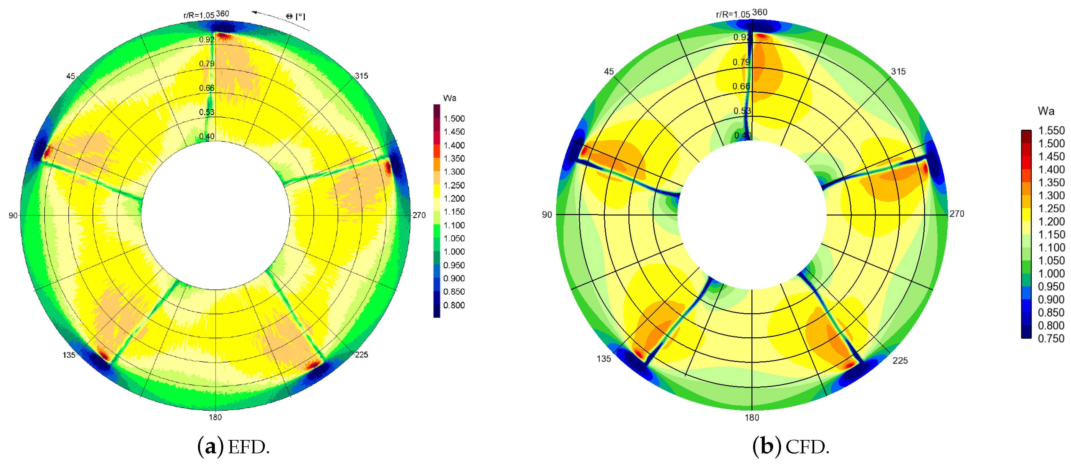
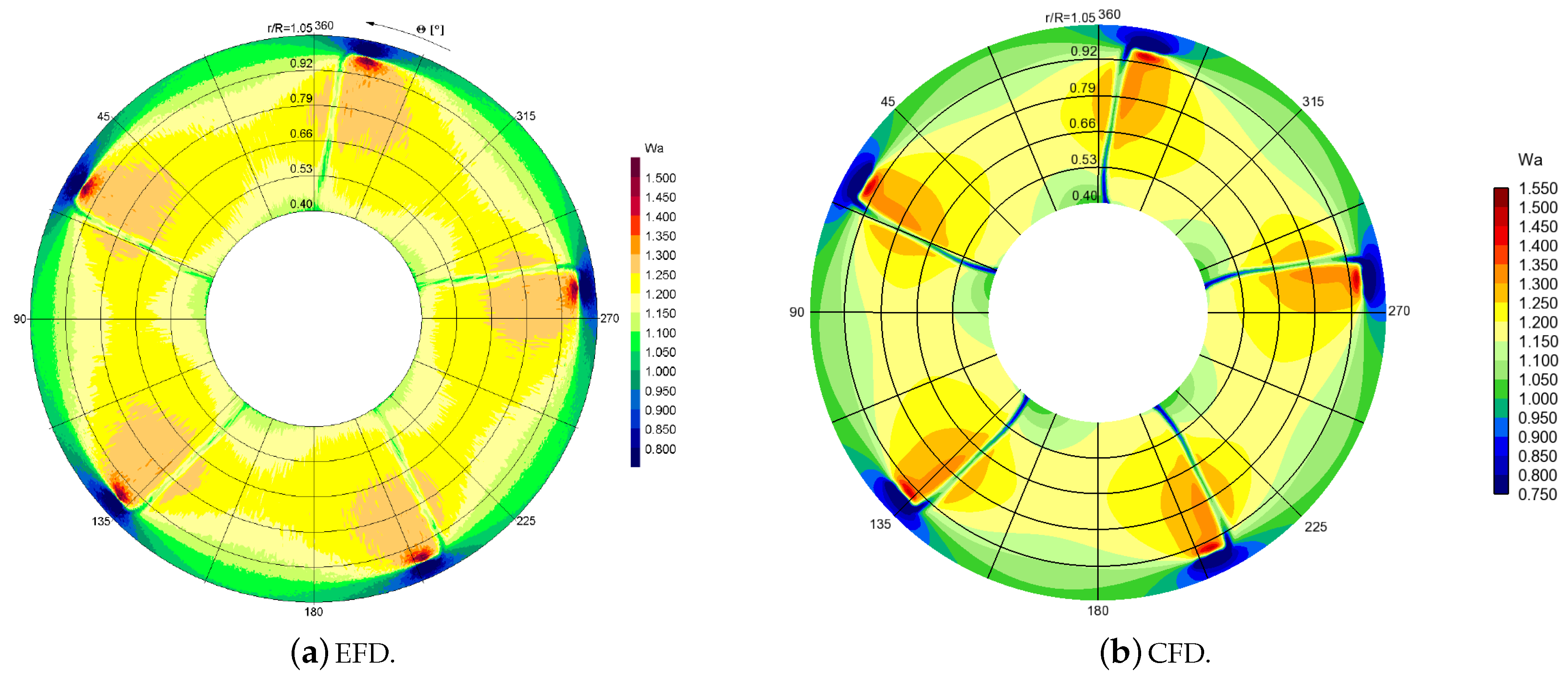
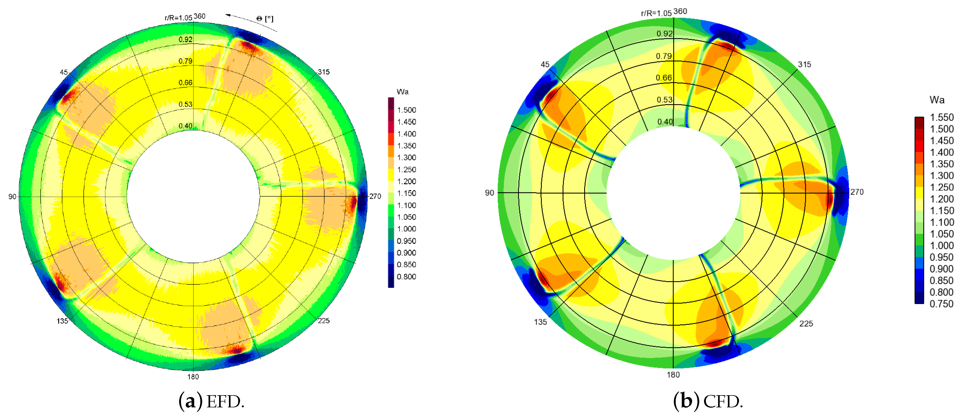
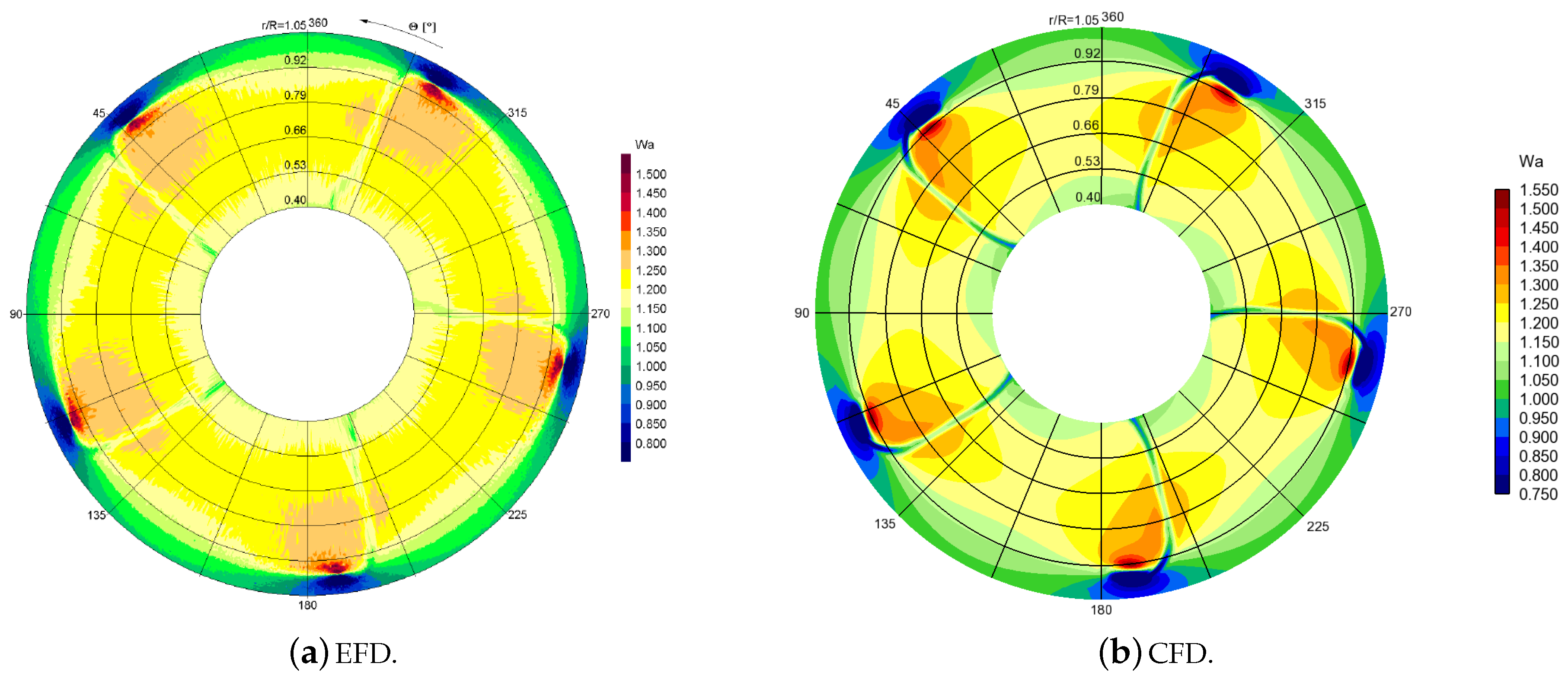
Next, we compare the axial wake of the propeller to the LDV measurements conducted in a cavitation tunnel. The measurements were made at non-cavitating conditions at
, and the comprehensive LDV experimental results were reported by Mach [
53]. The axial wakes at four axial distances from the propeller plane were compared, namely on the plane
in
Figure 8, on the plane
in
Figure 9, on the plane
in
Figure 10, and on the plane
in
Figure 11.
Comparing the EFD and CFD axial wake distributions, it can be seen that overall the propeller wakes were mostly very similar between CFD and the experiments. The accelerated flow region on both sides of the thin decelerated blade wakes were also clearly present in the simulations. The spatial evolution of the blade wakes and associated flow patterns around them were also well captured in the simulations, including the form and strength of the tip vortices. The axial velocity distribution near the tip vortices was very similar, although the simulations predicted the maximum local wake at a slightly lower radius than was observed in the experiments. In addition, the simulations predicted a somewhat larger velocity deficit for the thin blade wakes. We note that the small deviations between the present simulations and the experiments were in line with observations made during the smp’11 workshop (
http://www.marinepropulsors.com/proceedings-2011.php), where several CFD codes were compared with the LDV measurements.
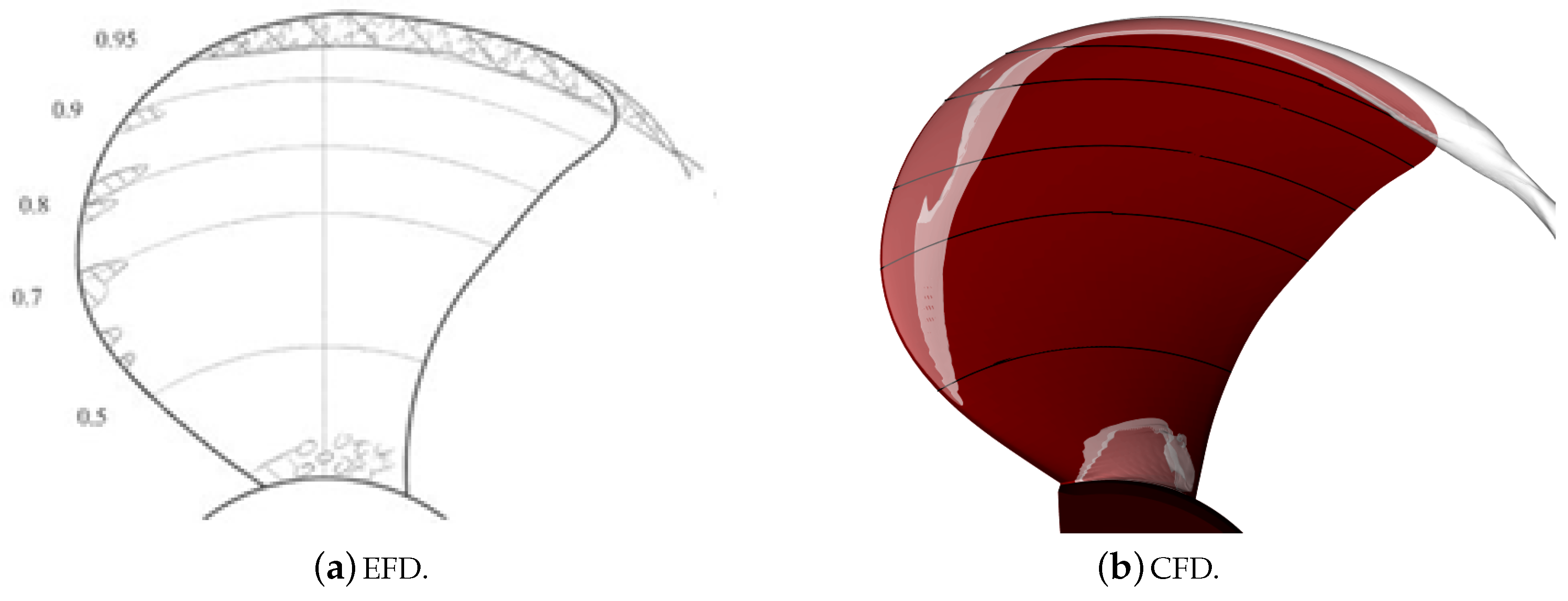
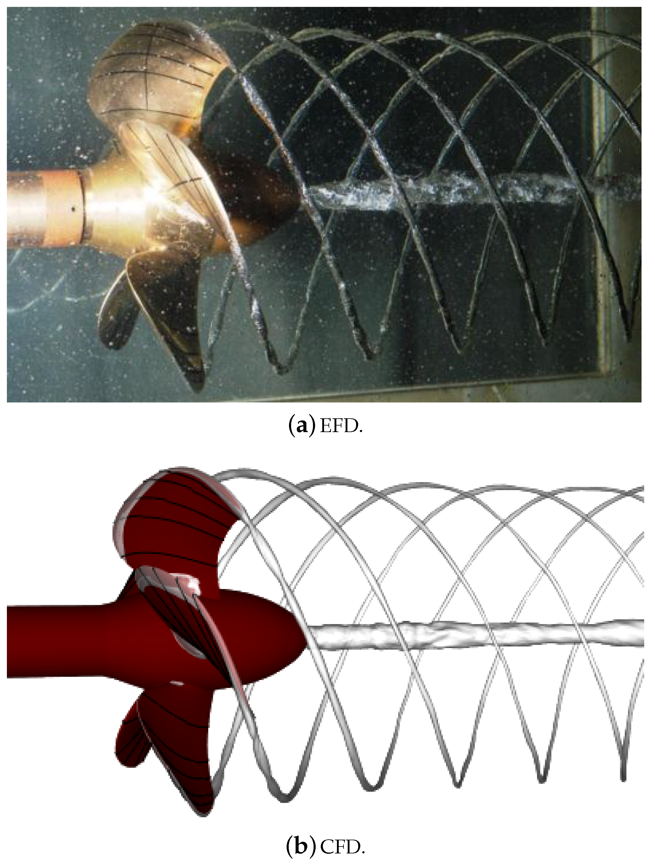
Figure 12 and
Figure 13 show the cavitation patterns at
on the suction side of the propeller blades as well as in the propeller wake together with the observations made in the cavitation tunnel tests. The propeller has strong tip vortex and hub vortex cavitation, which was visible in the experiments and in the simulations. Shedding of root cavitation was observed in the experiments and in the simulations. It should be noted that the unstable behaviour was very mild in the simulations. Otherwise, the shape and extent of the root cavitation, as well as the tip and hub vortex cavitation, were captured well. The tip and hub vortex cavitation extending far behind the propeller were captured exceptionally well, as shown in
Figure 13. Comparing the EFD and CFD results in
Figure 13, it can be seen that the modal shapes of the cavitating tip vortex were also qualitatively well-captured. Furthermore, streak cavitation in the experiments at several radial locations near the leading edge of the blade was identified, while the simulation predicted sheet cavitation at the leading edge.
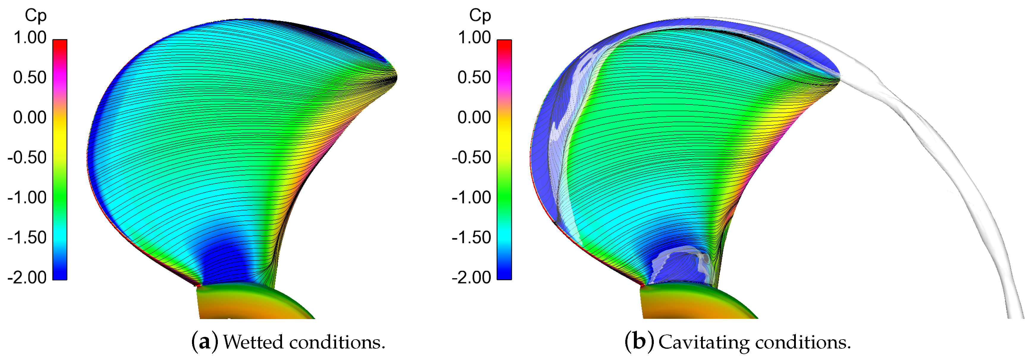
The surface restricted streamlines and pressure coefficients,
, on the blade surface in wetted and cavitating conditions, are shown in
Figure 14. The boundary layer flow was mostly circumferentially directed along the blade. The effect of cavitation on the surface restricted streamlines was significant. The re-entrant jets were directed towards the cavitating tip vortex at the closure line of the sheet cavitation,
cf. Refs. [
25,
49]. In addition, flow separation was visible in the blade root region at cavitating conditions, caused by the blade root cavitation. Furthermore, the wetted case computation predicted a more radially extended although relatively fine separation region at the trailing edge of the blade.
5.2. Wake Flow Structures
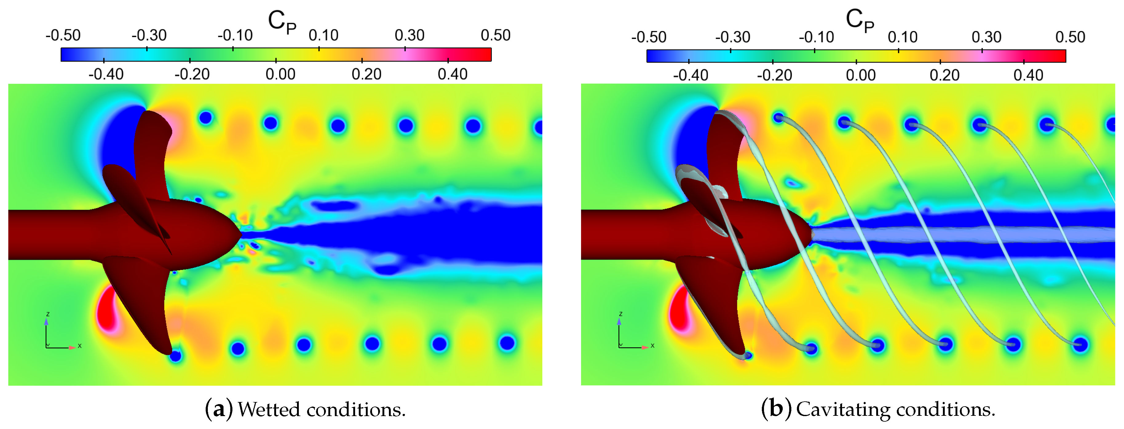
The pressure coefficient near the propeller and in its wake is visualized in
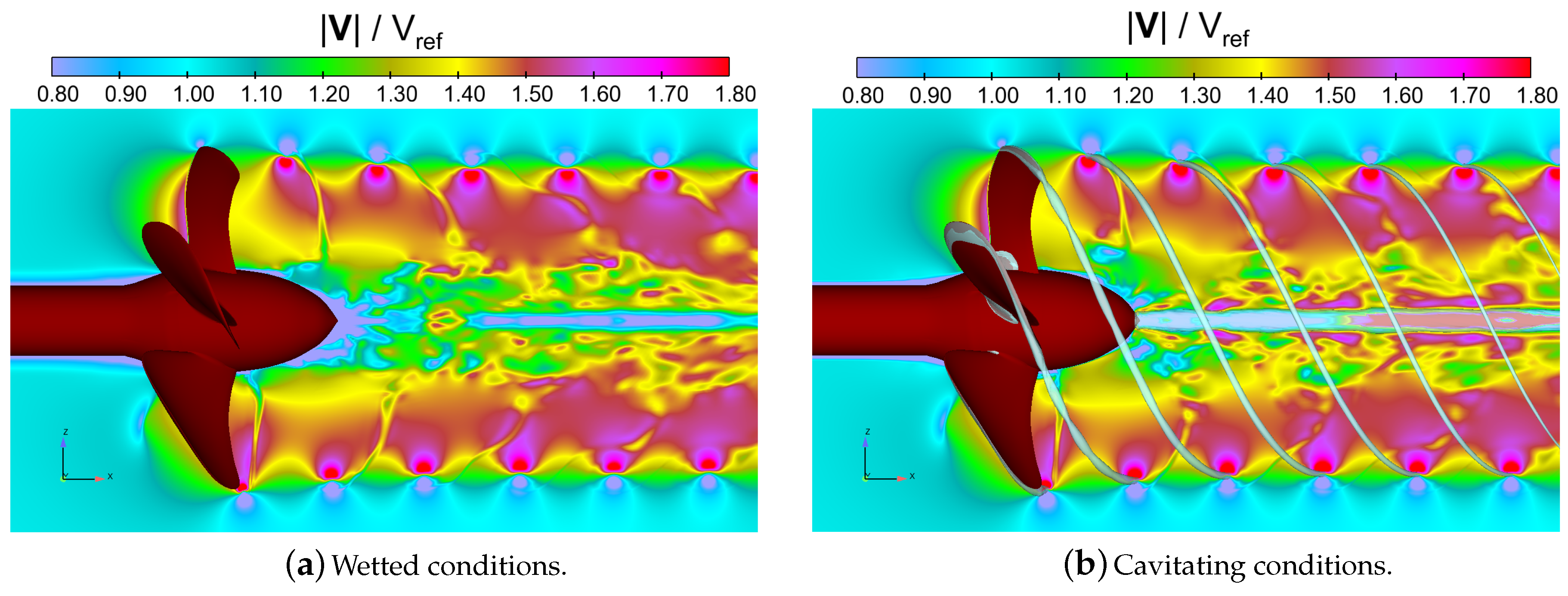
Figure 15. In the figure, we compare the wetted and cavitating conditions. A corresponding comparison of the magnitude of non-dimensional velocity (
) is shown in
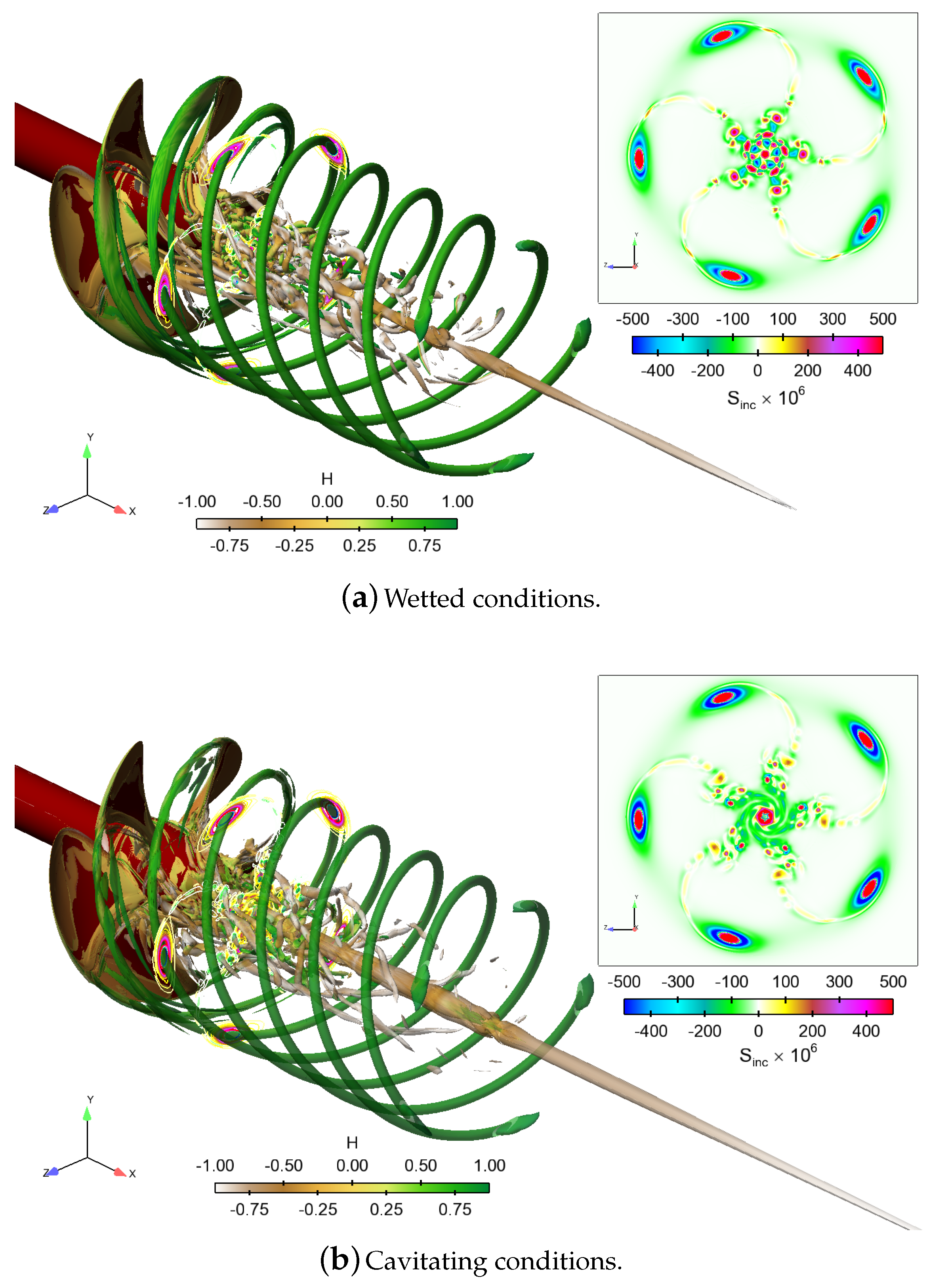
Figure 16. It can be seen that the strong tip vortex was preserved well in the slipstream. In both the wetted and cavitating cases, the flow field near the tip vortex region was convected far in the wake, nearly unaffected by the distance it travelled. Dissipation of flow disturbances in the tip vortex region was low, and the tip vortices were well preserved up to the extent of the helical grid.
In
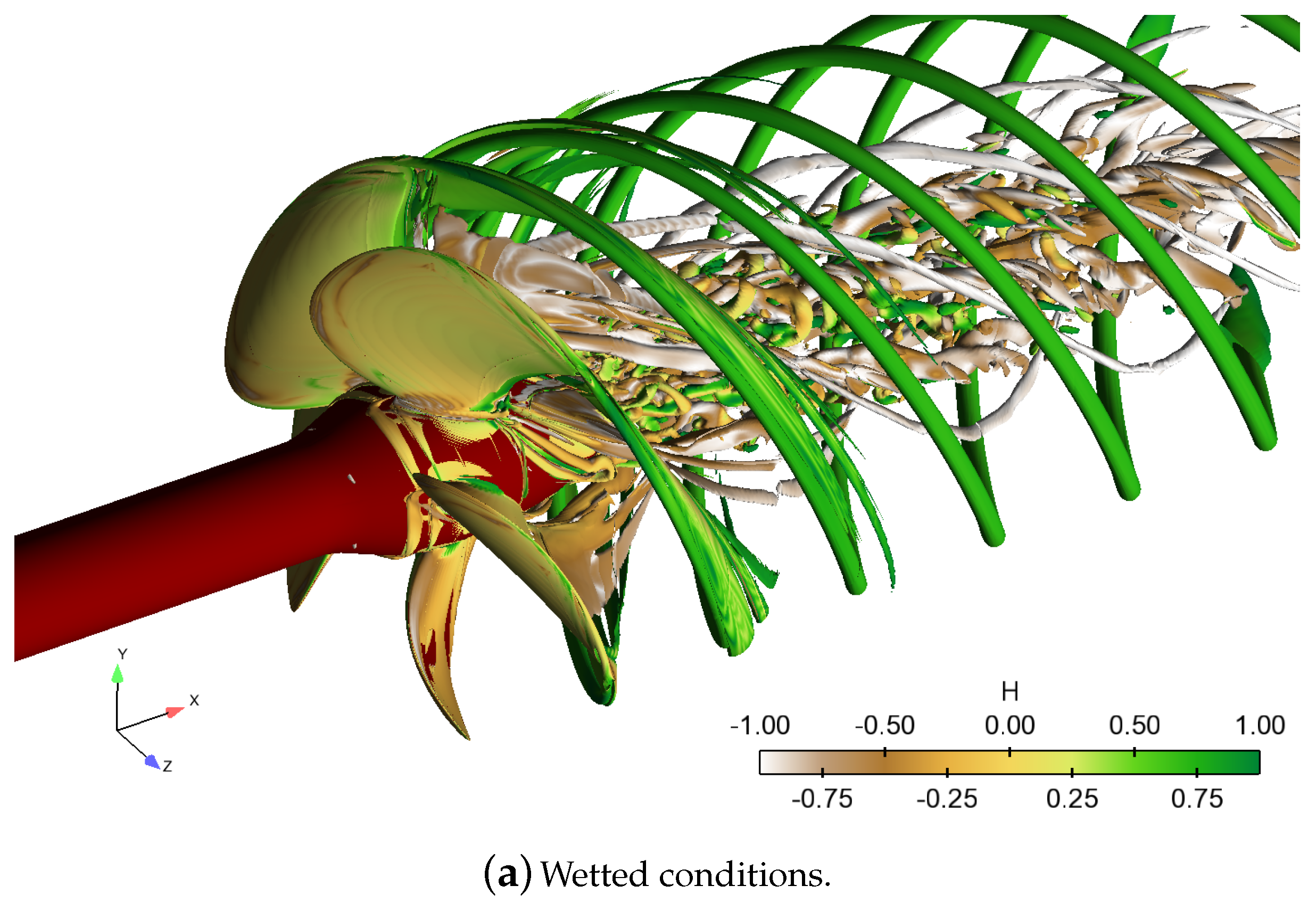
Figure 17, the flow field near the propeller is visualized by an iso-surface of the second invariant of the velocity gradient tensor, or the
Q criterion. The iso-surface had the value of
, and it was coloured by helicity
, where
is the relative velocity vector in the rotating reference frame. The helicity denotes the cosine of the angle between the relative velocity and the absolute vorticity vectors, and tended to
in the vortex cores, the sign indicating the direction of swirl. Several distinct areas characterized by different types of vortical flow structures were seen in the wake of the propeller in both the wetted and the cavitating cases. Distinct, regular, and strong vortical flow structures with dominant vorticity direction aligned with the flow were due to the tip vortices caused by the blades. As was noted above, these convect with little dissipation up to the extent of the helical grid. The modal shapes of the cavitating tip vortex are also seen in
Figure 17b. At small radii behind the propeller hub, the wake was dominated by the vortical flow structures shed by the hub in both cases. This also had a relatively regular structure, in addition to being strong enough to maintain cavitation up to the extent of the helical grid,
cf. also
Figure 12. Flow structures that originate from the root of the blade then again differed more between the wetted and cavitating conditions. In the wetted case, several horseshoe-type vortical structures being shed in the wake existed, whereas in the cavitating case, the wake structures did not appear as clearly. Furthermore, distinct flow patterns originated from near the midspan of the blade. In the wetted case, as the blade wake departed the blades, the vortical flow structures seemed to converge to a distinct vortex filament which then coiled as a helical shape with its vorticity aligned with the flow (i.e.,
). Similar structures were present in the cavitating simulations, but with less clarity of the helical composition; closer observation near the trailing edges of the blades revealed that the vortical structures caused by the blade boundary layer destabilized just after the trailing edge (TE) for the cavitating case. These differences were due to the leading edge cavitation as well as the enhanced flow separation from the root section of the blades in the cavitating conditions, since the relatively stable root cavitation caused the flow separation (
cf. Figure 14) as observed also in previous studies [
25,
37].
5.3. Acoustic Excitations
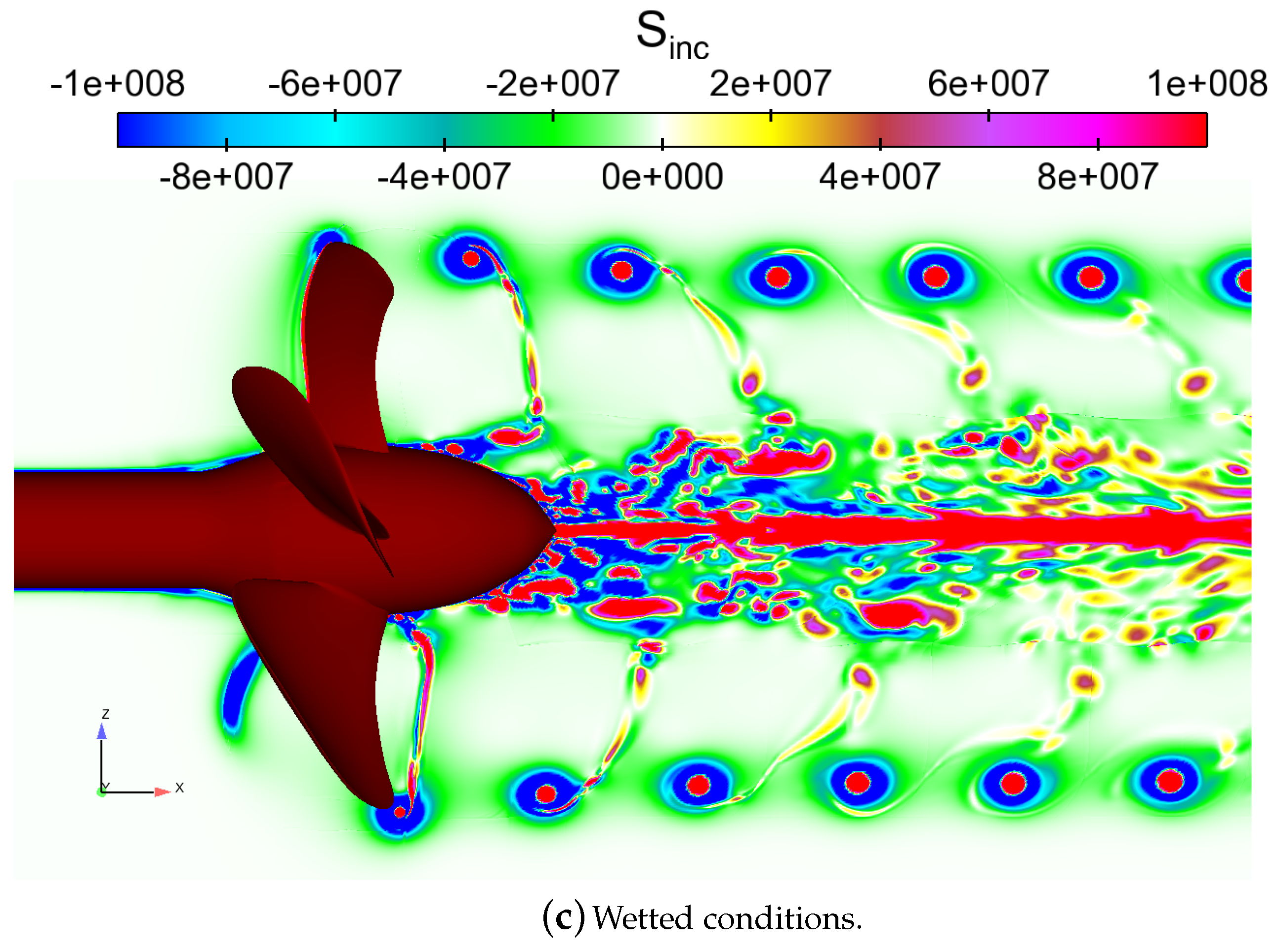
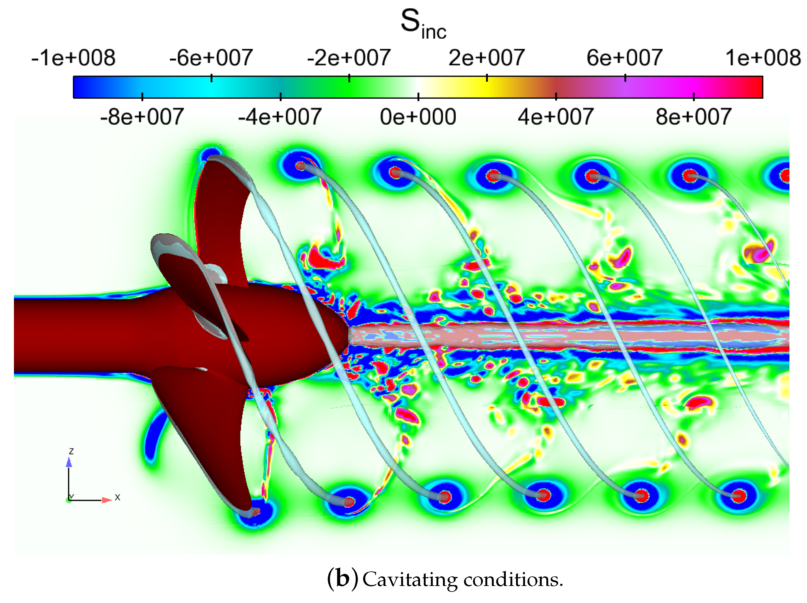
Figure 18 shows the acoustic source terms obtained from the CFD solution on the cut plane
utilizing different turbulence models in wetted conditions. As shown by Saarinen and Siikonen [
56], the divergence of the divergence of the Lighthill tensor, or the source term of the acoustic wave equation, can in incompressible cases be simplified to
, where
Q is the second invariant of the velocity gradient tensor.
Figure 19 furthermore shows the acoustic source terms, obtained from the CFD solution, on the plane
for the wetted and cavitating cases. The figure also shows the vortical flow structures in terms of the
Q criterion, together with contours of the acoustic source term on the plane. We can see that in the wetted case, the acoustic source term distribution was more concentrated and regular near the hub vortex than in the cavitating case. In the cavitating case, the source distribution was spread to a slightly wider radius in the wake. For instance, the presence of the helical vortex filament that was shed behind the blades in the wetted case can be seen in the acoustic source term distributions. The tip vortex structure was slightly different between the wetted and cavitating conditions, and in the cavitating case around the elongated core of the tip vortex a larger area of negative source region was present.
The sound pressure can be very sensitive to the location of the investigation point in the propeller near-field. The sound field characteristics in a wave guide (e.g., a cavitation tunnel) depend considerably on the type of the source, in addition to its position and orientation, as concluded in Hynninen et al. [
36]. To overcome this problem, in this paper, the mean square pressure over the cavitation tunnel domain was used to compare the results. A comparison of the mean square pressure inside the cavitation tunnel, in wetted and cavitating conditions, is shown in
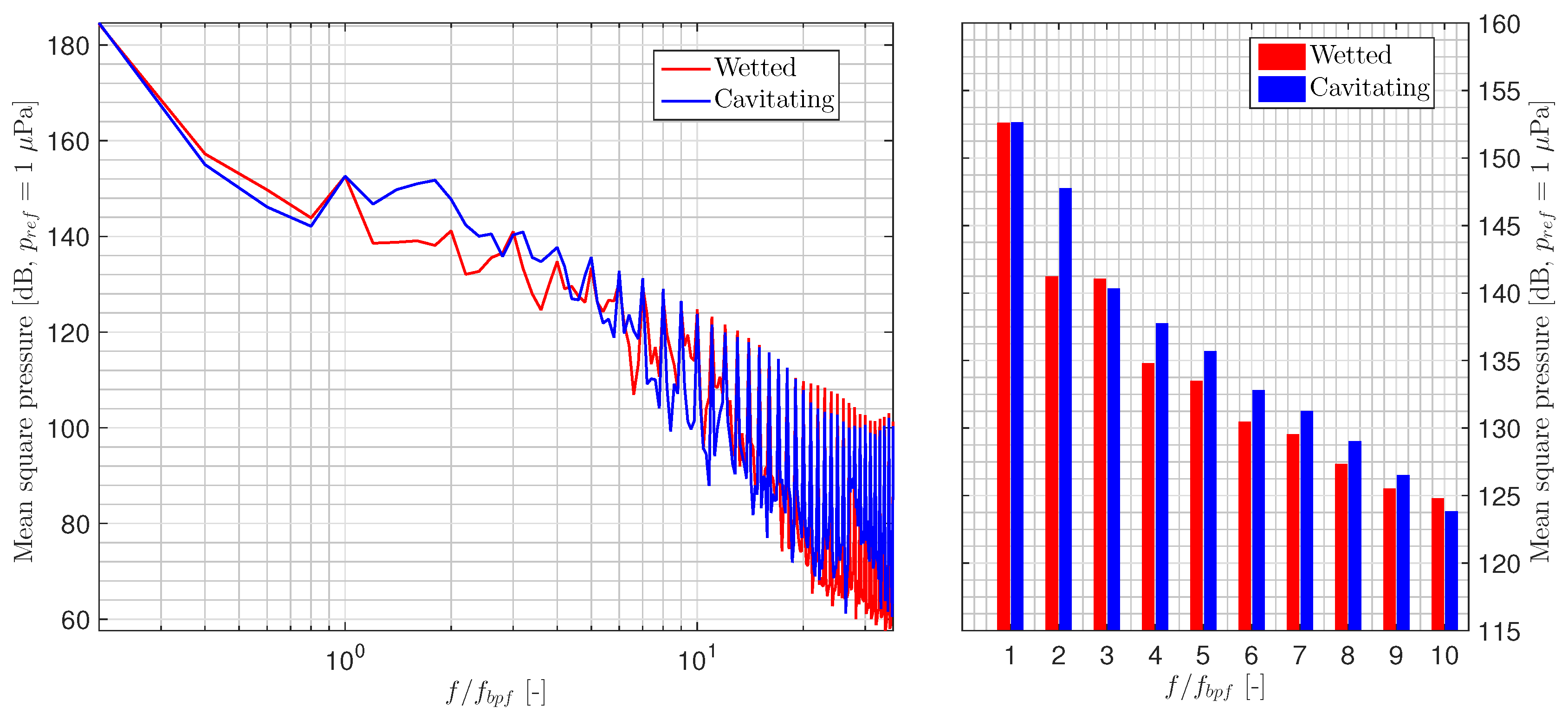
Figure 20. Additionally, the figure shows a corresponding comparison of the mean square pressure at the first ten blade passing frequencies. The results were obtained from the CHA simulations.
In both investigated cases, the acoustic excitation was high at discrete frequencies at the blade passing rate and its harmonics. A difference of more than 10 dB between the and its second harmonic was observed in the wetted case, whereas in the cavitating case, we noted a corresponding difference of approximately 5 dB. We observed that cavitation resulted in greater acoustic excitation at the low-frequency range from and at the high-frequency end of the investigated range. Additionally, the sound pressure levels at the harmonics of the blade passing frequency were on average at a higher level for the cavitating case. Then again, at frequencies between tonals 8 10, the non-cavitating case exhibited a greater acoustic excitation.
An increase in the predicted mean pressure levels was visible at around
27 in the cavitating case. The observed behaviour is due to the fact that an unsymmetrical tunnel mode was excited—a phenomenon which is discussed by Hynninen et al. [
36]. For broadbanded frequencies higher than
27, the cavitating case had larger acoustic excitation. The relatively equal level of acoustic sound pressures at the blade passing rate then again presents a new issue, as previous simulations with the SST turbulence model coupled with an EARSM (explicit algebraic Reynolds stress model) [
37] predicted higher acoustic excitations at the BPF for the cavitating case. This must be further investigated in the future.
In the studied wetted case, flow separation near the blade root or at the hub was not extensive. Flow around the blades behaved smoothly, and also the wake flow structures appeared somewhat clearer. In the cavitating case, the computations also predicted a rather stable root cavitation, which caused apparent changes to the flow geometry that led to separation near the trailing edge. This introduced instabilities in the wake as well, some being more prominent than those we observed in the wetted case. Consequently, an increased level of broadband noise was induced due to cavitation.
6. Conclusions
We have presented results of a hybrid CFD–CHA study of a marine propeller in a cavitation tunnel. DDES was used to obtain a transient solution of the propeller flow and wake dynamics, and an acoustic Lighthill analogy was used in the FEM context to simulate the propeller-induced acoustic propagation.
The predicted open water characteristics of the propeller were close to the experimental results, although the simulations had the tendency to under-predict the thrust and torque. Good agreement was observed between the numerically simulated propeller wake patterns and experimental LDV measurements, with the tip vortex evolution and other relevant wake flow details captured with the numerical simulations. Cavitation patterns were also well predicted, and the cavitating tip and hub vortices were excellently captured with the DDES.
However, if we are mainly investigating the global propeller performance characteristics, utilization of higher-fidelity turbulence closures is not always justified due to also the higher computational burden they impose. Then again, if one aims to resolve important vortical and cavitating flow structures and turbulent flow patterns also in the propeller wake, the choice of appropriate turbulence modelling approach becomes a key question. For such situations, hybrid RANS/LES type approaches offer attractive alternatives to the propeller two-phase flow simulations.
In the propeller noise simulations, a two-step hybrid approach was used. An examination of the CHA results with respect to the CFD-simulated flow field indicated that the sound pressure levels were reasonable, and effects due to cavitation were recognized. It was seen that the propeller wake could act as an acoustic source in a wide frequency range, while cavitating tip vortex enhanced the higher-order tonal signature. However, validation of the present acoustic simulations with experimental results is still needed. Yet, the comparison of single-point measurements conducted in a cavitation tunnel and the acoustic simulations is not straightforward. Sound pressure can be very sensitive to the location of the investigation point in the propeller near-field. The sound field characteristics in a wave guide (e.g., a cavitation tunnel) depend considerably on the type of the source, in addition to its position and orientation. The transformation of the results to corresponding free-field values is difficult. These issues are thoroughly discussed by Hynninen et al. [
36].
A grid dependency study for the acoustic analyses is needed. In addition to evaluating the CFD sources from coarser and finer grids for the CHA, the sensitivity of the predicted noise levels to the numerical approximation used in the FEM should be investigated. To further improve the flow solution for smaller turbulent fluctuations and possible cavity instabilities, a finer temporal resolution could be utilized in the present DDES.
Cavitation also contributes to the acoustic excitation due to the source term related to the density variations. A scale-resolving turbulence modelling approach further enhances the predictions of the wetted and cavitating propeller-emitted noise as it aims to resolve, instead of to model, the turbulent flow fluctuations. In order to capture the possible broadband noise contribution due to rapidly varying cavities, special attention needs to be given to the cavitation modelling apart from the present compressible flow solution algorithm. Currently, mass-transfer models are used which are based on a pressure difference
, on its square root or other similar relation. One option to improve the cavitation modelling would be a multi-scale two-phase flow model, such as that developed by Hsiao et al. [
57]. The flow solution can be further developed by assuming unequal velocities for the phases [
58]. This creates new challenges for the modelling of turbulence and interfacial transfer, which will be important research topics in the future.


