Abstract
In common model testing practise, the measured values of the self propulsion test are split into the characteristics of the hull, the propeller and into the interaction factors. These coefficients are scaled separately to the respective full scale values and subsequently reassembled to give the power prediction. The accuracy of this power prediction depends inter alia on the accuracy of the measured values and the scaling procedure. An inherent problem of this approach is that it is virtually impossible to verify each single step, because of the complex nature of the underlying problem. In recent years the scaling of the open-water characteristics of propeller model tests attracted a renewed interest, fuelled by competitive tests, which became the norm due to requests of the customer. This paper shows the influence of different scaling procedures on the predicted power. The prediction is compared to the measured trials data and the quality of the prediction is judged. The procedures examined are the standard ITTC 1978 procedure plus derivatives of it, the Meyne method, the strip method developed by the Hamburgische Schiffbau-Versuchsanstalt (HSVA) and the -method by Helma.
1. Introduction
The International Towing Tank Conference ITTC established the “1978 ITTC Performance Prediction Method” (ITTC 1978) [1], which is widely used to extrapolate the data collected during model test to full scale performance for trial or service condition. In recent years, it was suggested by more and more people—mainly designers of unconventional propellers—that the predictions made using this method often do not reflect the performance measured during ship trials, see for example Brown et al. [2]. Most authors believe that these deviations between prediction and measured performance is due to the scaling method for the open-water performance, which is needed by the ITTC 1978 power prediction method. Consequently, they either modified the ITTC method or came up with completely new methods (Praefke [3] and Helma [4,5]).
Since the performance of a full scale propeller is not easily available, Helma [4,5] suggested to scale the open-water data from tests performed at different Reynolds numbers to the full scale propeller, arguing that a good scaling method must give the same results for all model-test Reynolds numbers. It also mentions that the final validation should be done by comparing predicted with measured performance data, which is the topic of this paper.
2. Scaling Methods for Propellers
Currently, the following scaling methods are described in the literature:
- Statistical methods
- Analytical methods
- CFD methods
- Combinations of the above methods
2.1. Statistical Methods
Statistical methods try to match the measured data to the full scale performance by a relation derived by statistical analysis.
2.1.1. ITTC 1978 Method
The best known statistical propeller scaling method is described in ITTC’s Performance Prediction Method (ITTC 1978). The origin of this method is described by Kuiper [6] “as based on statistics and the basis for the statistical values is very small”. This method correlates the change in the thrust and torque coefficients and to the change in the section drag of a significant section profile, the chord length to diameter ratio , the number Z of propeller blades and the pitch to diameter ratio . The section drag again depends on the thickness to chord length ratio and the Reynolds number calculated with the section length c. According to the ITTC 1978 method, the integral characteristic of the propeller blade is substituted by a significant section located at a fractional radius of .
As long as the propeller to be scaled falls into the envelop of the propellers used in the statistical analysis, this method gives good results. Nevertheless it should be mentioned that this method introduces a dependency of the lift coefficient of the significant profile on the pitch to diameter ratio (see also Appendix A). The authors believe that this behaviour does not capture the underlying physics.
Another disadvantage can be seen in the fact that the method does not take the camber distribution of the sections into account, resulting in a lower correction for propellers with higher cambers.
2.1.2. Derivatives
Based on the same statistical approach, some authors tried to improve the accuracy of the ITTC 1978 method by using different form factors and friction lines [7].
2.2. Analytical Methods
Analytical methods derive the section’s lift and drag coefficient and from the measured open-water data. There are two approaches described in the literature.
2.2.1. Meyne Method
The method of Lerbs/Meyne [8] addresses propeller performance scaling in combination with a propeller analysis step, which is lifting line based. It gives access to a hypothetical open-water performance of the propeller valid for a non-viscous fluid. In comparison with the experimental open-water results, specific friction corrections are obtained for model scale, while global friction adjustments are done for the full scale propeller. These are based on an equivalent profile assuming that the integral values of the whole blade are reasonably well reflected by the singular value of this profile. Meyne suggested to use the profile located at .
It should be mentioned that this method assumes that the propeller analysed has an optimum circulation distribution with minimum losses. An immediate result is that this method does not work as well for propellers with a non-optimum circulation distribution, such as propellers restricted in diameter or tip-unloaded propellers.
2.2.2. -Method
Helma [4,5] showed that the mean hydrodynamic inflow angle into an equivalent profile can be calculated from the open-water test as follows:
where the factor
is a purely geometric constant depending only on the ratio of the hub to propeller diameter .
With this result, the measured thrust and torque can be split into the lift and drag of the equivalent profile, which can be scaled independently. In the last step of the calculation, they are combined again to the scaled thrust and torque figures.
The advantage of this method is the decomposing into the lift and drag coefficients, which are aligned with the hydrodynamic inflow and not the nose-tail pitch line. It also does not assume any special circulation distribution or a form drag of the section, but it still works on the assumption of an equivalent profile.
2.3. CFD Methods
The direct numerical simulation (DNS) represents the most accurate computational approach to describe surface friction effects, but is too expensive for scaling purposes. The large eddy simulation (LES) truncates the scales which are to be resolved to describe turbulent flow, but remains too costly when used with the exact propeller geometry. The RANS method reduces the required resolution in time and space further by introducing empirical turbulence models at all scales. RANS results are sensitive to grid qualities, turbulence modelling options and implementation details of the actual computer code. There is more work to be done until the RANS method gives repeatable results independent of the code used and the programme’s operator.
2.4. Combined Methods
2.4.1. HSVA’s Strip Method
The strip method was proposed as early as 1994 by Praefke [3] and recently deployed by HSVA [9]. It should cover any blade shape, because surface friction effects are treated in an integral manner by dividing the blade into strips covering all sections between the hub and the tip. A section drag coefficient is dedicated to each strip depending on the local Reynolds number.
2.4.2. Numerical Section Drag
A boundary layer solver might be linked with a potential flow solver to calculate section drag including effects ignored by the friction lines mentioned previously, see Thwaites [10], Head [11] or Drela [12].
3. Section Drag
With the exception of the CFD-based and the Meyne methods, all methods rely on the a priori knowledge of the drag coefficient of the propeller section profiles, either for a significant section or for all sections, which are subsequently integrated over the blade. According to Abbot and Doenhoff [13], the drag of a two-dimensional section can be composed of the frictional drag of one side of a flat plate and a drag increase , due to the shape of the section, which can be written in coefficient form as
where the indices u and l denotes the upper and lower faces of the section.
Whereas the frictional resistance coefficient depends solely on the Reynolds number and the relative roughness (with k the finished roughness of the propeller), the form drag shows a complicated relationship to the thickness to chord ratio , the Reynolds number, the relative roughness and also .
3.1. Viscous Drag of a Flat Plate
Generally speaking, two flow regimes can be observed:
- Laminar flow and
- turbulent flow.
Depending on the Reynolds number, the inflow turbulence and the surface condition of the flat plate, the flow might become turbulent while travelling along the flat plate, leading to a laminar-turbulent transition zone. The following cases can be observed:
- Laminar case:
- The flow is laminar over the entire plate. The viscous drag decreases with increasing Reynolds number.
- Transition governed case:
- The flow starts to become turbulent. The higher the Reynolds number, the earlier this transition occurs. Since the viscous resistance of a turbulent flow is higher than that of a laminar flow, the frictional drag increases with higher Reynolds numbers.
- “Fully” turbulent case:
- If the transition point moves close to the leading edge, the influence of the laminar flow on the overall drag diminishes and the viscous drag decreases again with an increase in the Reynolds number.
The frictional resistance of the laminar flow follows a simple correlation to the Reynolds number. However, open-water tests of propellers are conducted around Reynolds numbers of and , thus putting them into the transition region. Real size propellers work well above a Reynolds number of , generally around 5 ×, subjecting them to fully turbulent flow.
It is theoretically possible to calculate the frictional resistance of a hydrodynamically smooth flat plate for laminar and fully turbulent flow. For one side of the plate these are given as local skin friction coefficients as follows:
Laminar region:
Turbulent region:
where is the Reynolds number based on the distance x from the leading edge; is the Reynolds number based on the boundary layer thickness at x; and , B and are constant factors suitably selected.
The behaviours of the friction lines discussed are shown in Figure 1.
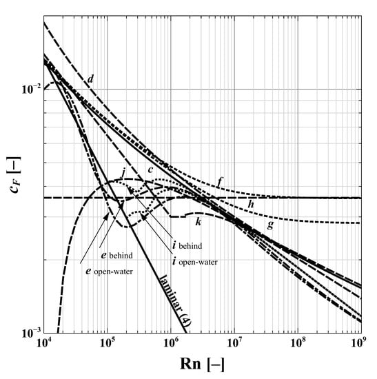
3.1.1. Friction Line for Laminar Flow
Equation (4) can be readily integrated to give the normalized frictional drag for one side of the whole plate:
3.1.2. Friction Line for Fully Turbulent Flow
For the turbulent flow, Equation (5) gives implicitly in terms of . To make matters worse, the Reynolds number used in this context depends on the local boundary layer thickness , which is not known. There were many approximations given for both coefficients and , some are listed in Table 1. Some of them are based on a theoretical model and some are curves fitted to experimental data, which might explain the differences in these lines. Five relationships do not explicitly include the relative roughness , whereas the ITTC 1978 and two more general friction lines take the surface finish into account.

Table 1.
Exemplary values mentioned in the literature for the viscous drags and for one side of a flat plate with fully turbulent flow. The first five relationships assume a hydrodynamically smooth surface, the others take the relative roughness of the surface into account.
It must be noted that the Streckwall et al. friction line e includes the form drag (see Section 3.2).
3.1.3. Friction Lines for Transition Region
The two friction lines presented in Equations (4) and (5) are only valid if the flow is either laminar or turbulent over the whole length of the flat plate. Strictly speaking, this is only possible for laminar flow, since each turbulent flow starts near the leading edge as laminar flow and trips to turbulent instantaneously at the transition point. With the Reynolds number increasing, this transition occurs relatively closer to the leading edge. For high enough Reynolds numbers, this contribution of the laminar region gets so small that it can be neglected; the flow can be considered fully turbulent and calculated accordingly.
The distance of the transition point from the leading edge depends not only on the local Reynolds number, but also on the surface quality of the plate, the turbulence of the inflow and—in the case of profiles—the chord wise pressure gradient. These factors pose a formidable challenge to calculate a universal friction line for the transition region.
Some friction lines found in the literature are given in Table 2. It is noteworthy that none of these takes the surface roughness of the plate or the turbulence of the inflow into account, which depend on the common practice followed by the testing facilities. It can be assumed that the relationships given by ITTC 1978 and Schulze (d, j and k) include these effects in a general way (for the ITTC 1978 line) or for one special towing tank (the Schulze line). The transition line i as used by Streckwall et al. integrates the local friction coefficients and for the laminar and turbulent flow over the length of the plate. It assumes that the transition occurs at the position from the trailing edge. This formulation would result in a discontinuity of the boundary layer thickness at the transition point. For this paper, this formulation was improved in such a way that the local Reynolds number for the turbulent flow was adapted, so that in the transition point the impulse loss thickness is the same for the laminar and the turbulent boundary layer (Schlichting [14]).
Table 2.
Exemplary values for the viscous drag of a flat plate mentioned in the literature. is the position from the leading edge along the plate where the flow trips from laminar to turbulent a.
3.2. Form Drag
The form drag is the increase of the drag of a two-dimensional section when compared to the purely viscous drag of a flat plate. The reason for this increase is two-fold: Firstly, the flow velocity over the surface is higher due to the thickness of the profile increasing the viscous drag. Secondly, the pressure does not recover entirely due to losses in the boundary layer:
where is the relative increase of the friction due to the speed increase and is the drag coefficient due to pressure losses.
The increase of the friction due to the higher velocity depends on the relative speed increase, the position of the transition point and the pressure gradient along the profile. For symmetrical sections, the speed increase is the same for both sides and only depends on the thickness to chord ratio . The position of the transition point depends on the Reynolds number, the turbulence of the inflow and the section shape. Values found in the literature for symmetrical profiles are given in Table 3.
Table 3.
Values for the relative form drag for symmetrical section profiles mentioned in the literature. For the NACA 64 and 65 laminar profiles, the transition point was fixed at . Hoerner also emphasised that the given relationship for these sections are only valid for rough surfaces [18].
The pressure drag coefficient can only be determined by analysing experimental results. It can be argued that it also depends on the position of the transition point, the pressure gradient and the occurrence of separation. Some values found in the literature for symmetrical profiles without flow separation are given in Table 4.
Table 4.
Values for the relative pressure drag for symmetrical section profiles without flow separation mentioned in the literature. See also explanations given for Table 3.
4. Section Lift
Abott and von Doenhoff remarked in their book that the turbulent lift coefficient of aerofoils changes only minimally with the Reynolds number [13]. There are claims that this observation does not hold for propellers, e.g., Bugalski et al. [20], who also gave a formula for the lift coefficient as a function of the Reynolds number. This possible influence of the Reynolds number is not included in the current investigation.
5. Methodology
Since full scale open-water performance data for propellers are not easily attainable, the most straight-forward approach is to compare the power and shaft revolutions predicted from model tests with the values measured during full scale trials:
where and are model–ship correlation factors for the power and shaft speed, respectively; and are measured and predicted delivered power, respectively; and and are measured and predicted shaft revolutions, respectively.
If the prediction methods were perfect, these two model–ship correlation factors would be 1 for every model test analysed However, it is to be expected that these factors scatter around a mean value, which is not necessarily 1. This shift in the mean value can be corrected by applying the model–ship correlation factor as a final step in the power prediction, as stated in the ITTC 1978 method. A measure of the scatter is the standard deviation, which assumes that the distribution of values forms the bell shaped curve. The smaller the standard deviation the closer are the scattered values to the mean value, hence the better is the scaling method. Note that, before calculating the standard deviation, the values must be normalized to give a mean value of 1.
The analysis was run by the Hamburgische Schiffbau-Versuchsanstalt (HSVA).1
HSVA currently uses the strip method and previously used the Lerbs/Meyne [8] and the standard ITTC 1978 [1] methods, so these were already available. The -method was implemented by Stone Marine Propulsion (SMP), just as the ITTC method. This was necessary, so that the ITTC method can be used with different friction lines and form factors, which were implemented by SMP as well. Using this newly developed program, it was possible to calculate the open-water characteristics for the self-propulsion and full scale conditions for all possible combinations of scaling methods, friction lines and form factors.
Based on HSVA’s databases of performance predictions and sea trials, the intersection of both sets was identified. The expected power was calculated according to HSVA’s standard performance prediction method [9].
The 25 scaling methods used are summarized in Table 5. The finished roughness k of the propeller in full scale was assumed to be 20 m.
Table 5.
Scaling methods investigated. A mark in the ∫-columns denotes that the scaling procedure integrates the sectional friction over the whole blade. The capital letters specifying the friction lines, form and pressure drag are references to the Table 1, Table 2, Table 3 and Table 4, respectively (OW, open-water; SP, self-propulsion; and FS, full scale). The finished roughness k of the propeller in full scale was assumed to be 20 m.
5.1. Performance Prediction Method
At HSVA, self-propulsion is simulated via the so-called Continental Method. Model speeds are to be converted to full scale following Froude’s similarity law. Under self-propulsion, the hull model is additionally towed by a force to compensate for increased surface friction effects present in model scale. The 1957 ITTC friction line is used to prescribe a hull surface friction coefficient (to be applied to the wetted surface) in model and full scale [17]. depends on the difference in surface friction and the evaluation process solely involves the difference without any form factor entering. A correlation allowance (a function of the vessel’s length and its block coefficient) is added instead to evaluate . covers added resistance of the zinc anodes, standard hull roughness and small openings. Assuming a complete geometrical similarity and disregarding any superstructure, the model scale thrust would be directly convertible to full scale. However, the full scale prediction of the shaft speed needs a prediction of the actual full scale effective wake fraction and the Yazaki’s method [21] is applied for this purpose. As usual, to allow for a trial prediction, the normalized propeller thrust measured behind the model is enlarged to account for air resistance of the superstructure and (if necessary) to include appendages and hull openings not present during the model tests. The thrust correction causes adequate power and shaft speed adjustments for the sea trials, achievable by the aid of the propeller open-water diagram.
5.2. Analysis
The intersection of performance predictions and sea trials available at HSVA consisted of 360 data records (see Table 6). For 183 records, the open-water characteristics could not be calculated for all scaling methods considered. By visual inspection it was found that three sets have an obvious mistake in either the available trial or prediction data. The remaining 174 datasets consist of 38 unique propeller-hull configurations. The mean values of and were calculated for each of these configurations using each of the 25 propeller scaling methods listed in Table 5. Finally, the resulted distribution was filtered according to Tukey’s range test: If for one dataset more then half of the values are outside Tukey’s range calculated with the typical value of , this dataset was disregarded. The Tukey’s range for valid data points was calculated with:
where and are lower and upper quartiles of all values for one scaling method , respectively. Applying this test yields a total of 35 ships to be included in the evaluation. The range of ships are shown in Table 7.
Table 6.
Number of used datasets.
Table 7.
Range covered by the 35 ships included in the final analysis.
Using these 35 valid datasets, the following values were calculated for each scaling method :
- Mean value of all datasets for each scaling method :
- Normalized model–ship correlation factors:
- Standard deviation of all normalized datasets for each scaling method :where N is the number of valid datasets and is the model–ship power correlation factor for the i-th dataset. Note that the normalized mean values are always 1.
The normalization (Equation (12)) of the model–ship correlation factors is necessary, because the ITTC power prediction method defines the model–ship correlation factors as multiplication factors (compared to an offset to be added) and the standard deviation changes, whenever the underlying data-set is multiplied by a constant factor. Without the normalization, it would favour scaling methods with smaller values.
6. Results
The mean values of the model–ship power correlation factors for each propeller scaling method (Equation (11)) are shown in Figure 2. It should be noted that a mean value of 1 is not necessarily an indicator for the quality of the propeller scaling method.
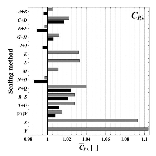
Figure 2.
Mean values of the model–ship power correlation factors for all scaling methods . If the same scaling method was investigated with and without scaling to the Reynolds number of the self-propulsion test, the results are grouped together; the black bar stands for the no scaling to the self-propulsion test. The capital letters reference Table 5.
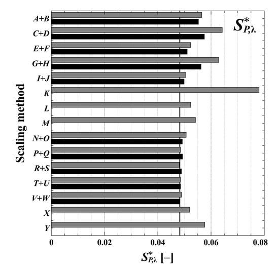
Figure 3.
Standard deviation of the normalized model–ship power correlation factor for all scaling methods . If the same scaling method was investigated with and without scaling to the Reynolds number of the self-propulsion test, the results are grouped together, the black bar stands for no scaling to the self-propulsion test. The capital letters reference Table 5.
- The mean values of the model–ship power correlation factor is about 1 for most investigated scaling methods.
- The scaling methods which do not scale down to the Reynolds number of the self-propulsion test typically perform better than the same method using the scaled down open-water characteristics to analyse the self-propulsion test (B–A, D–C, F–E, H–G, J–I, O–N, Q–P, U–T and W–V, but not S–R).
- The methods using the original Schlichting friction line f for the full scale propeller tend to perform better (E–A, F–B, G–C, H–D, T–P and W–S, but not U–Q and V–R).
- All methods using the local surface friction i trying to capture the transition from laminar to turbulent flow do not perform very well (K, X and Y).
- The -methods integrating the friction forces over the whole blade perform better than the same method using only the friction force of a significant profile (R–P, S–Q, and W–U, but not V–T and the notable exception Y–X). For the ITTC 1978 methods, this trend is reversed (C–A, D–B, G–E and H–F).
- The most recent methods perform better than the original ITTC 1978 method A.
- The -methods R and W integrating the ITTC 1978 and Schlichting friction lines h and f over the whole blade perform best, closely followed by other -methods using different approaches regarding the handling of the viscous resistance. The next best method is the HSVA strip method in a version O, which does not scale down to the Reynolds number range of the self-propulsion tests.
7. Discussion
The scaling approaches compared in this paper rely on the estimates of the normalized drag forces experienced by either a single section representing the blade or—in the integral cases, such as the strip method—by individual sections building up the blade. All methods but the Meyne and -methods consider the resistance force vector to be orientated in the direction of the nose-tail line; both the Meyne and the -method calculate the direction of the hydrodynamic inflow and aligns the resistance force parallel to it. In terms of a favourable standard deviation of the normalized power correction factor , the quality of a specific approach is also linked to the qualities of the drag estimates achieved in model or full scale. The ability to account correctly for local Reynolds number variations, either in the model or full scale Reynolds number region, would be reflected in a lower standard deviation.
Generally, it can be considered more challenging to capture Reynolds number sensitivities in the model scale case due to the extended presence of laminar flow over the model propeller blade. Referencing item 2 from the list presented in Section 5, it could be concluded that none of the used friction lines is able to predict the friction forces in model scale accurately. Better results are achieved by using the open-water data without any correction applied to analyse the self-propulsion test. One possible reason for this behaviour might lie in the fact that the inflow into the propeller during the self-propulsion test is more turbulent due to the boundary layer of the ship model than during the open-water test. This turbulent inflow would trigger an earlier transition from laminar to turbulent flow similar to the open-water test in undisturbed inflow.
The data presented indicate that for full scale the original Schlichting friction line f might be a good choice for any scaling procedure.
One has to be aware that not only the propeller scaling method has an influence on the predicted power and shaft revolutions: The favourable settings for arriving at the target will depend on other corrections entering the set-up and evaluation of propulsion tests. In particular the scaling of hull resistance and effective wake are to be mentioned in this context. It should be noted that more important than a value of unity is a small standard deviation. The offset of the mean value can be compensated for, whereas the standard deviation is a measure of the spread of predicted values, which should be kept small.
It should be mentioned that the strip method N has the advantage to have been confirmed previously by quite the same dataset used in this investigation to analyse all scaling methods.
All propeller scaling methods investigated in this paper are supposed to show negligible differences in view of their influence on the full scale shaft speed prediction. Consequently, the isolated sensitivity of the shaft speed forecast on the traditional propeller scaling approaches is to be considered minor. This can be shown by calculating the ratios
where is the model–ship correlation factor for the shaft speed calculated using the ITTC 1978 propeller scaling method A. A ratio close to 1 for all propeller scaling methods indicates a minor sensitivity of , which is shown in Figure 4 for all 177 valid datasets used in this investigation. This confirms that the predictions for the shaft speed are hardly a matter of propeller scaling contrary to the power predictions. The causes of this behaviour would justify an investigation on its own.
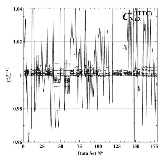
Figure 4.
of the model–ship shaft speed correlation factors normalized with the ITTC 1978 propeller scaling methods. The small scatter around the value of 1 indicates a small influence of the propeller scaling method on the prediction of the shaft speed.
8. Conclusions
The power and shaft revolutions were predicted by the standard HSVA performance prediction method but with 25 different propeller scaling methods. These predictions were compared to the measured trials data to quantify the quality of each propeller scaling method. The standard deviations of the normalized model–ship power correlation factors were calculated as a measure of the quality of the prediction. All investigated methods showed a mean value of this correlation factor of about 1.
Typically, better results can be expected if the open-water propeller characteristics are not scaled down to the Reynolds number of the self-propulsion test. A possible reason is explained in Section 6, but its cause should be investigated thoroughly, e.g., by paint tests and measuring the turbulence of the inflow into the propeller in open-water and behind condition. Finally, either a Reynolds number for the open-water test should be established, which results in the same flow pattern as in the self-propulsion test, or a friction line should be developed, which takes into account the increased turbulence of the inflow behind the ship model.
From the data available, the most promising friction line for the full scale propeller is the original Schlichting line f.
From the propeller scaling methods investigated, the -method in its variants R and W, where the friction forces are integrated over the whole blade, showed the best results. The most likely reason is that this method aligns the drag forces with the actual hydrodynamic inflow angle experienced by the propeller blade and that it does not need to know the sectional form drag.
It might be worthwhile to investigate numerical methods to calculate the section drag, such as outlined by Thwaites [10] and Head [11]. Drela implemented the transition from laminar to turbulent flow in the software XFoil [12]. The values for the section drag calculated numerically can be used by any scaling method investigated in this paper.
It must be mentioned that the original 360 trial datasets were reduced to just 35 unique propeller–hull combinations due to rigorous data checks and averaging over sister-ship cases. HSVA is currently investing in a maintenance program for the database to allow for an enlargement of datasets, which would pass the rigorous consistency checks.
With more data available, it becomes feasible to run an optimization on a parametrized friction line with the target to further minimize the scatter of the model–ship power correlation factors.
In the current investigation, the influence of different formulations of the form and pressure drags was not investigated.
Finally, it must be noted that no unconventional propellers, such as end-plate, tip-raked propellers or propellers with unconventional section shapes, such as the NPT propeller, were present in the datasets available to the current investigation. Because of the underlying physical principles, it can be assumed that the -methods integrating the friction forces over the whole blade will also perform best for these propellers. When unconventional propellers are included in such investigations, one should be aware that their number is very small compared to more conventional designs, hence their influence on the overall outcome is most likely negligible. Since most newly developed propeller scaling methods claim to give more accurate results for unconventional propellers, this group of propellers must be looked at separately to isolate the effect of different propeller scaling methods.
9. Final Note
The software developed to calculate the scaled open-water characteristics is published with an open license on the principal author’s GitLab website https://gitlab.com/sphh/PyOWscaling. All functionality are realized as plug-ins written in Python. It is easy to write your own plug-in to implement other propeller scaling methods, friction lines and in- and output formats. It would be appreciated if you made your plug-ins available to the public.
Author Contributions
The idea of this paper emerged during discussions between S.H. and H.S. J.R. set up and ran the power predictions. H.S. contributed the computer code for the strip method, parts of the manuscript, preliminary post processing and evaluated the data filtering. Stephan Helma contributed the computer code for the other scaling methods. He did the data filtering, the final post processing and wrote most of the manuscript.
Conflicts of Interest
The authors declare no conflict of interest.
Abbreviations
The following abbreviations are used in this manuscript:
| CFD | Computational Fluid Dynamics |
| DNS | Direct Numerical Simulation |
| FS | full scale |
| HSVA | Hamburgische Schiffbau-Versuchsanstalt GmbH |
| ITTC | International Towing Tank Conference |
| ITTC 1978 | ITTC Performance Prediction Method [1] |
| LES | Large Eddy Simulation |
| OW | open-water |
| SMP | Stone Marine Propulsion Ltd. |
| SP | self-propulsion |
| RANS | Reynolds-averaged Navier-Stokes [equations] |
Appendix A Review of ITTC 1978 Scaling Procedure
The total propeller force F can be composed from the propeller thrust T and torque Q
where x = fractional lever of the torque, which does not change with the scaling.
This relation can be made dimensionless by dividing by :
Using the ITTC 1978 [1] scaling for and
it is possible to scale the propeller force coefficient:
Hence
which shows that the scaled propeller force is not only a function of the thrust and torque figures and the increase in section drag , but also of the pitch to diameter ration . In the opinion of the authors this dependency cannot be explained with first principles. This surprising result is a property of all scaling methods which are based on the ITTC procedure.
References
- Performance Prediction Method. ITTC—Recommended Procedures and Guidelines; Effective Date 2014, Revision 03; ITTC: The Hague, The Netherlands, 1978. [Google Scholar]
- Brown, M.; Sanchez-Caja, A.; Adalid, J.G.; Black, S.; Sobrino, M.P.; Duerr, P.; Schroeder, S.; Saisto, I. Improving Propeller Efficiency through Tip Loading. In Proceedings of the 30th Symposium on Naval Hydrodynamics, Hobart, Tasmania, Australia, 2–7 November 2014. [Google Scholar]
- Praefke, E. Multi-Component Propulsors for Merchant Ships—Design Considerations and Model Test Results. In Proceedings of the SNAME Symposium (Propeller/Shafting’94), Virginia Beach, VA, USA, 20–21 September 1994. [Google Scholar]
- Helma, S. An Extrapolation Method Suitable for Scaling of Propellers of any Design. In Proceedings of the Fourth International Symposium on Marine Propulsors (Smp’15), Austin, TX, USA, 4 June 2015. [Google Scholar]
- Helma, S. A scaling procedure for modern propeller designs. Ocean Eng. 2016, 120, 165–174. [Google Scholar] [CrossRef]
- Kuiper, G. The Wageningen Propeller Series; MARIN: Wageningen, The Netherlands, 1992. [Google Scholar]
- Schulze, R. Neue Verfahren zur Reynoldszahlkorrektur für Freifahrtmessungen an Modellpropellern. Presented at the STG-Sprechtag, Moderne Propulsionskonzepte, Hamburg, Germany, 16 June 2016. [Google Scholar]
- Meyne, K. Untersuchung der Propellergrenzschichtströmung und der Einfluss der Reibung auf die Propellerkenngrößen; STG-Jahrbuch: Hamburg, Germany, 1972. [Google Scholar]
- Streckwall, H.; Greitsch, L.; Müller, J.; Scharf, M.; Bugalski, T. Development of a Strip Method Proposed as New Standard for Propeller Performance Scaling. Ship Technol. Res. 2013, 60, 58–69. [Google Scholar] [CrossRef]
- Thwaites, B. Approximate Calculation of the Laminar Boundary Layer. Aeronaut. Q. 1949, 1, 245–280. [Google Scholar] [CrossRef]
- Head, M.R. Entrainment in the Turbulent Boundary Layer. Aeronautical Research Council Reports. 1958. Available online: https://pdfs.semanticscholar.org/16b6/5a95963109996d23ce1f3e953fc493939f9e.pdf (accessed on 28 February 2018).
- Drela, M. XFoil Subsonic Airfoil Development System. 2013. Available online: http://web.mit.edu/drela/Public/web/xfoil/ (accessed on 28 February 2018).
- Abbott, I.H.; von Doenhoff, A.E. Theory of Wing Sections; Dover Publications, Inc.: New York, NY, USA, 1959. [Google Scholar]
- Schlichting, H.; Gersten, K. Grenzschicht-Theorie; Springer Verlag: Berlin, Germany, 2006. [Google Scholar]
- von Kármán, T. Turbulence and Skin Friction. J. Aeronaut. Sci. 1934, 1, 1–20. [Google Scholar] [CrossRef]
- Schönherr, K.E. Resistance of Flat Surfaces Moving Through a Fluid. Trans. Soc. Nav. Archit. Mar. Eng. 1932, 40, 279–313. [Google Scholar]
- Resistance Test. ITTC—Recommended Procedures and Guidelines; Effective Date 2011, Revision 03; ITTC: Kongens Lyngby, Denmark, 1957. [Google Scholar]
- Hoerner, S.F. Fluid-Dynamic Drag, Theoretical, Experimental and Statistical Information; Hoerner Fluid Dynamics: Bakersfield, CA, USA, 1965. [Google Scholar]
- Torenbeek, E. Synthesis of Subsonic Airplane Design. The Netherlands and Martinus Nijhoff; Delft University Press: Delft, The Netherlands, 1992. [Google Scholar]
- Bugalski, T.; Streckwall, H.; Szantyr, J. Critical Review of Propeller Performance Scaling Methods, Based on Model Experiments and Numerical Calculations. Polish Marit. Res. 2013, 20, 71–79. [Google Scholar] [CrossRef]
- Yazaki, A. A Diagram to Estimate the Wake Fraction for a Actual Ship from a Model Tank Test. In Proceedings of the 12th International Towing Tank Conference (ITTC), Roma, Italy, September 1969. [Google Scholar]
| 1. | Data processing was done solely at HSVA and results on trial predictions related to the various propeller scaling approaches were kept anonymous. The anonymous results on trial prediction were exclusively stored in normalized form, meaning that the quality of power and shaft speed predictions were expressed by the two model–ship correlation factors and . |
© 2018 by the authors. Licensee MDPI, Basel, Switzerland. This article is an open access article distributed under the terms and conditions of the Creative Commons Attribution (CC BY) license (http://creativecommons.org/licenses/by/4.0/).