Abstract
Recent breakthroughs in the computer vision community have led to the emergence of efficient deep learning techniques for end-to-end segmentation of natural scenes. Underwater imaging stands to gain from these advances, however, deep learning methods require large annotated datasets for model training and these are typically unavailable for underwater imaging applications. This paper proposes the use of photorealistic synthetic imagery for training deep models that can be applied to interpret real-world underwater imagery. To demonstrate this concept, we look at the specific problem of biofouling detection on marine structures. A contemporary deep encoder–decoder network, termed SegNet, is trained using 2500 annotated synthetic images of size 960 × 540 pixels. The images were rendered in a virtual underwater environment under a wide variety of conditions and feature biofouling of various size, shape, and colour. Each rendered image has a corresponding ground truth per-pixel label map. Once trained on the synthetic imagery, SegNet is applied to segment new real-world images. The initial segmentation is refined using an iterative support vector machine (SVM) based post-processing algorithm. The proposed approach achieves a mean Intersection over Union (IoU) of 87% and a mean accuracy of 94% when tested on 32 frames extracted from two distinct real-world subsea inspection videos. Inference takes several seconds for a typical image.
1. Introduction
Deep learning techniques have attracted significant interest in recent times as they have produced impressive results on benchmark and real-world datasets across a wide range of computer vision tasks. While deep learning methods are gaining popularity, a number of key obstacles still persist. Most notably, deep learning methods typically require very large training datasets to achieve good results and significant amounts of computational memory are necessary during inference and training stages. While computational power is continually improving and is becoming less of a barrier, there is still a scarcity of high-quality labelled training datasets for many applications, and this is especially true for underwater imaging applications. Curating a dataset takes time and domain-specific knowledge of where and how to gather the relevant information, and it often involves a human operator having to manually identify and delineate objects of interest from real-world images. This is a tedious and time-consuming task considering that datasets of up to thousands—or even tens of thousands—of training images are required to build a robust and effective deep network.
Having good quality training data is arguably one of the most important elements of any machine learning system and this is particularly the case for deep learning methods. A number of large-scale datasets have been created to provide dependable training data and to assist algorithm designers when devising new deep learning techniques for classification, detection, and segmentation tasks. This paper is concerned with semantic segmentation, which is the task of assigning each pixel in the input image a class in order to get a pixel-wise dense classification. Common datasets that can be used for training deep networks for semantic segmentation include:
- Pascal Visual Object Classes (VOC) [1] is a ground-truth annotated dataset of images. The dataset is partitioned into 21 classes which cover objects such as vehicles, household objects, animals, and people. There have been several extensions to this dataset [2,3].
- Microsoft Common Object in Context (COCO) [4] is a large-scale object detection, segmentation, and captioning dataset. The COCO train, validation, and test sets, contain more than 200,000 images and 80 classes, which include various vehicles, animals, food items, and household objects.
- SYNTHetic collection of Imagery and Annotations (SYNTHIA) [5] is a collection of imagery and annotations which has been generated with the purpose of aiding semantic segmentation and related scene understanding problems in the context of driving scenarios. SYNTHIA consists of a collection of frames rendered from a virtual city under a wide range of lighting and environmental conditions. It includes classes for buildings, roads, cyclists, and cars amongst others. Since the imagery is synthetic in nature, the pixel-level semantic annotations are precisely known.
Road scene understanding/autonomous driving is a popular application area and there are several other datasets relating specifically to this topic, such as KITTI [6], Cityscapes [7], and CamVid [8]. While these datasets are incredibly valuable for developing methods capable of interpreting road scenes/detecting common everyday objects, they are not particularly useful when it comes to developing custom underwater imaging techniques for applications such as damage detection, biofouling assessments, fish detection, etc. There is an underwater dataset, known as the Underwater Lighting and Turbidity Image Repository (ULTIR) [9], which contains annotated images of various types of damage, such as cracks and corrosion, captured under a host of underwater visibility conditions, however, there is less than 100 images per damage class and this is not sufficient to train deep models. To help bridge this gap, this paper proposes the use of synthetic imagery to train custom deep networks that can then be applied to interpret real-world underwater imagery. The focus of this paper is on interpreting underwater imagery for two main reasons. Firstly, underwater imaging is often severely hampered by factors—such as poor visibility, challenging underwater light-field, floating particle matter, air bubbles, colour attenuation, poor image acquisition practices, etc.—which limit the ability of cameras to observe and record details in the scene, and consequently, the effectiveness of image analysis algorithms is impaired. With this in mind, methods that perform with credibility when applied to underwater images are particularly valued. Secondly, there is an acute lack of labelled datasets containing underwater imagery which makes it harder for researches to develop deep learning methods for underwater applications. In order to harness the power of deep learning methods for underwater applications, researchers must look at new sources of training data. This study demonstrates that photorealistic synthetic data can help in this regard. Synthetic image datasets have been developed and used to the train deep learning algorithms for detection and classification of underwater mines [10].
A virtual scene of an underwater inspection site is created, and from this, a large dataset of synthetic imagery is generated with accurate ground-truth information that reveals the exact composition of the scene. This large dataset is then used to train a deep fully convolutional neural network architecture for semantic pixel-wise segmentation. While semantic segmentation/scene parsing has long been a part of the computer vision community, a major breakthrough came in 2014 when fully convolutional neural networks (CNNs) were first used by Long et al. [11] to perform end-to-end segmentation of natural images. Their approach took advantage of existing CNNs which are designed for classification problems, such as AlexNet [12], VGG (16-layer net) [13], GoogLeNet [14], and ResNet [15]. These classification models learn high-level feature representations, however, instead of classifying based on these extracted features, the compact feature representations are upsampled using fractionally strided convolutions to produce dense per-pixel labelled outputs. Fully convolutional neural networks allow segmentation maps to be generated for input images of any size and are faster than previous patch-based deep learning approaches. They also achieved a significant improvement in segmentation accuracy over traditional methods on standard datasets like Pascal VOC while preserving efficiency at inference. Many of the leading techniques that have emerged since Long et al.’s breakthrough work are also based on fully convolutional neural networks. A comprehensive review of deep learning techniques for semantic segmentation is provided by [16].
The performance of deep learning methods depends on the architecture of the deep network. Using an existing network/architecture, which is known to work well, as the basis for training new deep networks is usually a good strategy. In this paper, we adopt an existing architecture known as SegNet [17]. SegNet, which was originally developed for road scene understanding applications where it is important to obtain smooth segmentations between different classes such as roads and cars. As such, the network must have the ability to delineate objects and retain boundary information.
In this study, the SegNet architecture is adapted to detect biofouling on marine structures. Biofouling, which is sometimes referred to as marine growth colonisation, introduces several problems including increased hydrodynamic forces acting on structures, masking of structural components (thereby impeding the detection of defects such as cracks and corrosion), and the creation favourable conditions for biocorrosion [18]. Owners and operators of marine structures, therefore, need to track the progression of biofouling so that expensive cleaning regimes can be optimised and so that engineers and designers have more accurate estimates of the forces imparted by waves and currents. Ideally, a complete inspection of biofouling on a structure should be designed to periodically collect the following information: (i) identification of marine growth species (ii) percentage of surface covered by the main species, (iii) thickness of superimposed layers and their weight, and (iv) the average size of each species present on the structures. Identification of marine growth species is important as different species have different roughness characteristics and this affects how much energy is absorbed from passing waves and currents. Engineers must also know about the distribution of marine growth species on a colonised structure as this is a first step in computing more accurate loading estimates. Image-based semantic segmentation techniques can be especially helpful in providing information on both species identification and distribution. Moreover, underwater three-dimensional (3D) imaging techniques, such as [19], are well-suited for collecting in-situ measurements of the thickness and size properties of biofouling instances. With this in mind, imaging systems may be regarded as a convenient and standalone tool capable of collecting all of the necessary data for biofouling assessments [20].
Performing semantic segmentation on images of biofouling scenes is a challenge as, like many natural objects, marine growth species do not have consistent and well-defined shapes, and have non-uniform colour and textural properties. The reduced underwater visibility conditions add an additional layer of complexity to the detection problem [21]. To tackle this problem, this study creates a virtual scene of an underwater inspection site, and from this, a large dataset of synthetic imagery is generated with accurate ground-truth information that reveals the exact composition of the scene. This large dataset is then used to train a deep encoder–decoder network, which is applied to interpret real-world inspection imagery. This typically results in a good, albeit crude, segmentation. As an additional step to improve the quality of the segmentation, support vector machines are trained based on the initial segmentation map and boundaries of the detected biofouling regions are then iteratively refined using SVM classification so that the final segmentation map more closely aligns with the outline of objects in the scene.
2. Materials and Methods
The main steps involved in devising and evaluating the deep network for semantic segmentation is illustrated in Figure 1.
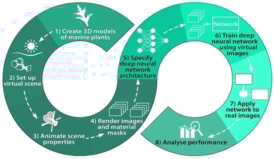
Figure 1.
Methodology of the proposed approach.
2.1. Create 3D Models of Marine Plants
The first step towards building a deep network capable of identifying biofouling in images is to create virtual 3D models of the marine growth species that we wish to identify. These 3D models should approximate the shape, colour, and texture of the real-world marine growth species that we are interested in. While it would be possible to have several different classes for various kinds of marine growth species, such as some of those shown in Figure 2, for the ease of demonstration, this case study will only focus on segmenting soft-fouling algae species from the background.
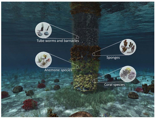
Figure 2.
Examples of other virtual marine species. The geometry and material properties can be easily adjusted.
It is important to note that the 3D models are not directly used as input when training the deep learning algorithm. Instead, the 3D models are scattered around a virtual underwater environment and thousands of synthetic images featuring the 3D models are rendered. It is these rendered images (along with the corresponding ground-truth per-pixel labels) that are used for training the deep learning algorithm.
Creating 3D models of marine growth species can be difficult in some cases, especially for complex marine species which have highly irregular and varied shapes. One way to combat this issue is to make use of the many 3D models that are available online—many of which are freely downloadable. It is often easier to download and customise these existing 3D models and incorporate them into the project rather than creating 3D models from scratch.
2.2. Set-Up Virtual Scene
Setting up the virtual scene involves simulating the underwater environment as realistically as possible. This mostly entails configuring the lighting and the optical properties of the water. This is carried out in VUE® which is a computer graphics software for creating, animating and rendering 3D environments. A view of the virtual scene is shown in Figure 3a. A real-world underwater scene is shown in Figure 3b for reference.
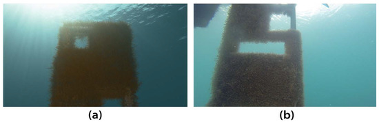
Figure 3.
View of a (a) virtual scene, and (b) real-world scene with the courtesy of MAPIEM, University of Toulon.
There is growing interest in creating underwater scenes for virtual reality (VR) applications, such as [22]. This is a burgeoning field and there can be strong crossover between developing underwater scenes for VR applications and for training deep models.
2.3. Animate Scene Properties
In order for a deep neural network to generalise well and to be successful when presented with new scenes, the network should be trained on a large and diverse dataset (i.e., a dataset consisting of thousands of images featuring varying lighting and visibility conditions, viewing perspectives, different plants from the same marine species category, etc.). For this case study, the created dataset consists of 2500 rendered images. It exhibits a high degree of diversity as several parameters of the virtual scene were animated (i.e., they evolved over time) to reflect many different conditions that may be encountered in a real-world setting. These parameters include:
- Properties of the underwater medium: transparency/visibility range and the colour of the water.
- The shape, size, and colour of the marine species.
- Species distribution on the structure’s surface. There were three scenarios here: sparsely populated, densely populated, and appearing in clusters.
- The intensity and nature of the on-site illumination (e.g., the position of the virtual sun was varied which gave rise to different lighting conditions).
- The position and orientation of the virtual camera in the scene—this produces images of the biofouling from a wide variety of viewing angles and camera–subject distances.
2.4. Render Images and Material Masks
Since a virtual scene was the source of imagery in this study, the process of populating the dataset with new images could be easily automated and new images could be added on-demand. The chief limiting factor on the number of images was the rendering time needed to produce each image. On average, it took approximately 50 s to render an image and the corresponding ground-truth class label image. The size of each image is 960 × 540 pixels. A sample of the rendered images and the ground-truth class labels is shown in Figure 4.
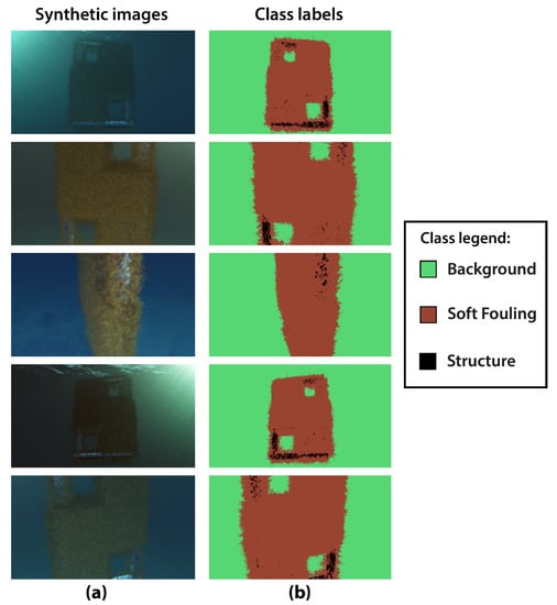
Figure 4.
Some examples of training imagery. (a) Sample imagery of a virtual marine growth scene, and (b) shows the corresponding ground truth labels—green indicates the background, black indicates the clean underlying surface of the structure, and brown indicates marine growth.
For this case study, the ‘background’ and the ‘structure’ class (with reference to the class legend in Figure 4) were combined into one class. Every pixel which was not deemed to represent biofouling regions was considered to be a member of the background class. These synthetic images and ground truth labels are passed onto the next stage and used to train the SegNet deep model.
2.5. Deep Model Set-Up
The encoder–decoder network used in this study uses the SegNet architecture. It consists of two separate deep neural networks: an encoder network and a decoder network. The encoder accepts an RGB (red, green, blue) image of size 960 × 540 as input and generates a high-dimensional feature vector. The decoder network then takes this high-dimensional features vector and produces a semantic segmentation mask that is the same size as the input image (960 × 540). The architecture of an encoder–decoder network is shown in Figure 5.
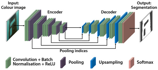
Figure 5.
The input to the encoder–decoder network is a colour image and the output is a semantic segmentation mask. Adapted from [17].
The encoder part of the network gradually reduces the spatial dimension with pooling layers. While this serves to aggregate the contextual information (i.e., the key features which reveal the scene composition), the precise location information of objects in the scene is eroded with each spatial down-sizing. However, semantic segmentation requires the exact alignment of class maps and thus, the location information needs to be preserved. The purpose of the decoder is to gradually recover the object details and spatial dimension. There are connections from corresponding pooling layers in the encoder to upsampling layers in the decoder which help the decoder to recover object details more effectively.
For this simple example, the encoder–decoder network is trained to predict whether each pixel in the input image belongs to one of two classes: the background or algae/soft biofouling. For more complex examples, there can be several classes (e.g., there can be a separate class for each marine growth species and the ‘background’ class can be divided into two classes—one class for the clean uncolonised surface of the structure and another for the background).
2.6. Deep Model Training
An inherent drawback of encoder–decoder networks and deep learning, in general, is that parameters of the neural networks must be learnt, and this requires very large datasets on which to train. Furthermore, the training times can take many hours or even days. For the demonstrated example, the training time was under 6 h using an 11 GB NVIDIA 1080Ti graphics card.
2.7. Application of the Trained Model to Real-World Data and SVM-Based Region Enhancement
Once trained, the encoder–decoder network is presented with new real-world images and tasked to perform semantic segmentation. The segmentation results for a sample image is shown in Figure 6.
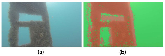
Figure 6.
(a) Input image, and (b) initial segmentation following application of SegNet with the courtesy of MAPIEM, University of Toulon.
It is evident from Figure 6b that while SegNet is effective at identifying the general location of biofouling regions in an image, it does not produce clean segmentations. A popular way to refine the segmentation is to apply a post-processing stage using a conditional random field (CRF). CRFs incorporate low-level pixel information with the output of segmentation methods to produce an improved segmentation which more closely coincides with edge boundaries of objects in the scene. For the proposed method, we adopt a support vector machine (SVM) based approach whereby SVMs are used to classify pixels at the boundary of biofouling regions in order to improve the size and shape characteristics of identified regions. Combining the deep encoder–decoder network and SVM enhancement in an effective manner creates a powerful yet expeditious segmentation method. The quick inference times of the SegNet technique (less than a second per image) is complemented by the strategic application of the higher complexity SVMs.
SVM is a supervised learning classifier based on statistical learning theory. The linear SVM is used for linearly separable data using a (f-1) dimensional hyperplane in f dimensional feature space [23,24,25]. This hyperplane is called a maximum-margin hyperplane which ensures maximized distance from the hyperplane to the nearest data points on either side in a transformed space. The linear kernel function is the dot product between the data points and the normal vector to the hyper-plane. The kernel function concept is used to simplify the identification of the hyperplane by transforming the feature space into a high dimensional space. The hyperplane found in the high dimensional feature space corresponds to a decision boundary in the input space.
In SVM, the classifier hyperplane is generated based on training datasets. For the proposed approach, the training data is the pixel colour information within the background and biofouling regions, as detected by SegNet in the preceding phase. Although some of the training data is likely to be incorrect since SegNet will rarely achieve 100% accuracy, it is expected that the vast majority of the training data will be appropriately labelled, and this will outweigh the relatively small number of errant training instances. Given a training dataset of l points in the form where h denotes the hth vector in the dataset, uh is a real f-dimensional input vector containing the mean and kurtosis values associated with each region and vh is an instance label vector ; for this example, a value of +1 indicates biofouling and −1 indicates the background, although SVMs can readily be extended to classify multiple classes using multi-class SVMs. To identify the maximum-margin hyperplane in the feature space, the SVM requires the solution of the optimization problem:
The function φ maps the training vectors into a higher dimensional space. The vector w is the weight vector which is normal to the hyperplane, e is the bias, ξ is the misclassification error and C is the cost or penalty parameter related to ξ. The solution to the problem is given by:
with constraints:
where K is the kernel function αh and αq are the Lagrange multipliers, vx,y is a label vector for the input point ux,y,c. where x and y are the horizontal and vertical spatial indices of the input image and c is the colour channel index. The linear kernel has been used here,
There is one preselected parameter value for the SVM, namely the cost parameter C, which may be optimised trial and error approach. A value of C = 1 was chosen and it was found the final results were not significantly affected by this parameter.
The enhancement process firstly examines pixels that are immediately adjacent to each class within the initial segmentation produced by SegNet. A pixel is considered to be adjacent to a region if it shares an edge or corner with any pixel on the periphery of that region. SVM classification is applied to these adjacent pixels utilising their original intensity values to classify each of these pixels as representing biofouling or the background. Pixels which are classified using SVMs as representing biofouling become a member of the region. This process is repeated until there are no more pixels that can be added to or removed from a region. The results following region enhancement are shown in Figure 7.
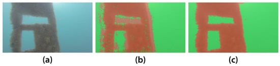
Figure 7.
(a) Original input image, (b) initial segmentation results following application of SegNet, and (c) final segmentation following SVM-based region enhancement with the courtesy of MAPIEM, University of Toulon.
It may be observed from Figure 7 that, following region enhancement, the segmentation is ‘cleaner’ and it coincides with the true outline of objects in the scene.
2.8. Performance Evaluation
Many evaluation criteria have been proposed to assess the performance of semantic segmentation techniques. Amongst the most common metrics are pixel accuracy and the Intersection over Union (IoU) scores. Pixel accuracy is simply the ratio between the amount of properly classified pixels and the total number of pixels in the image.
It is defined as:
where k is the number of classes, pij is the number of pixels of class i inferred to belong to class j, and pii represents the number of true positives, while pij and pji are usually interpreted as false positives and false negatives respectively (although either of them can be the sum of both false positives and false negatives).
The intersection over union, also known as the Jaccard Index, is the standard metric for segmentation purposes. It computes a ratio between the intersection and the union of two sets, in our case the ground truth and our predicted segmentation. That ratio can be reformulated as the number of true positives (intersection) over the sum of true positives, false negatives, and false positives (union). That IoU is computed on a per-class basis and then averaged.
The next section presents all of the quantitative results for the proposed method when applied to 32 real-world inspection images.
The ground truth segmentation for these 32 images is created by a human operator who manually identified the biofouling regions in each image. The visually segmented images act as the control and are assumed to show the true composition of the scene.
3. Results
The proposed method was applied to 32 frames that were extracted from inspection videos obtained at two underwater sites. A representative sample of the segmentation results is shown in Figure 8. The accuracy and IoU scores for each of the illustrated images can be viewed in Figure 9 by using the reference numbers provided.
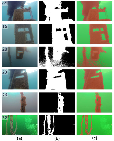
Figure 8.
(a) Input colour images extracted from underwater inspection videos, (b) detected biofouling regions, and (c) detected regions overlaid on the original input image with the courtesy of MAPIEM, University of Toulon.
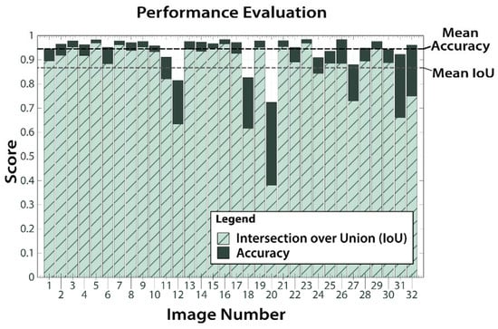
Figure 9.
Accuracy and Intersection over Union (IoU) scores for each of the 32 test images.
The performance of the proposed method, expressed in terms of accuracy and IoU scores, is illustrated in Figure 9 and the mean values are summarised in Table 1. The performances of two other techniques, which have previously been proposed in the domain of underwater imaging, are also included in Table 1. These techniques are a hybrid method called regionally enhanced multi-phase segmentation (REMPS) [26] and a texture analysis based segmentation technique [27]. Our approach achieves a mean Intersection over Union (IoU) of 87% and a mean accuracy of 94% when tested on 32.

Table 1.
Performance of the proposed approach along with other segmentation techniques previously proposed in the domain of underwater imaging.
It may be noted from these results that the proposed method was quite successful overall, and it proved effective at locating the presence of soft biofouling as well as accurately delineating biofouling regions in most cases. The major exception to this was image 20 (with reference to Figure 8 and Figure 9) where many background pixels were erroneously classified as representing biofouling. Closer inspection of this image reveals that there was a lot of small floating particles present in the water, especially in the lower half of the image where the rate of misclassification is most evident, and this may have contributed to the poor performance. These encouraging results support the idea that synthetic images can be a valuable source for training algorithms intended for real-world application. Furthermore, there is scope to improve the performance and usefulness of the proposed technique in several ways, including:
- Increasing the quantity and quality of the training data.
- Increasing the size of the input imagery. In the above example, the network accepts images of size 960 × 540 and outputs a segmentation mask of the same size. Being able to process higher resolution imagery (i.e., 1920 × 1080 pixels) would mean that the output segmentation masks could be more precise. Although the size of the input imagery is largely bounded by hardware constraints, in particular, the GPU.
- Having multiple classes for different marine species.
With regards to the last point, while it would be possible to have many different classes for several marine growth species (such as some of those shown in Figure 1), it may be better to group similar classes together. In practice, having many distinct classes is often more desirable and produces a segmentation technique of potentially greater utility than a segmentation technique that can only segment into two broader classes. However, having more classes can be problematic if there is high inter-class similarity within the training dataset. As an example, having separate classes for various types of marine growth species will be challenging in cases where there is a high degree of visual similarity between different marine species. In such cases, a better strategy may be to group similar classes together, i.e., have a ‘soft-fouling’ class that includes non-calcareous fouling organisms such as seaweeds, hydroids, and algae, and have another ‘hard-fouling’ class that includes calcareous fouling organisms such as barnacles, coral, and mussels. This will have the added practical advantage of reducing model training time. Moreover, having more classes also increases the likelihood of having unbalanced classes whereby the amount of training data in one category is less than other categories and this can impair the performance of the segmentation technique.
Finally, the model can be trained to suit the needs of the inspection since the virtual images can be generated on-demand (i.e., if the biofouling at an inspection site only consists of barnacles and seaweed then the encoder–decoder network need only include these classes).
Extension to Other Applications
The same concept of using virtual images to train an encoder–decoder for real-world application can be extended to other tasks, some of which are depicted in Figure 10. This is facilitated by the fact that deep learning models are highly repurposable. For instance, a model that is trained on a large dataset of marine growth images can be reused as a crack detection model by simply training the model on crack images instead, such as the study by Maeda et al. 2018 [28]. Very minor changes to the architecture of the model, if any, are necessary.
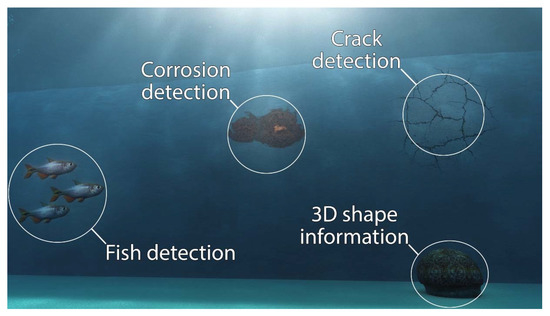
Figure 10.
Such data may be used to train an encoder–decoder crack detection model.
Additionally, marine biologists are often interested in detecting fish and estimating their size using camera systems. Being able to accurately detect fish, even in the presence of challenges such as overlapping fish and poor visibility, is of high value. Moreover, synthetic imagery is not only of value for semantic segmentation applications, it can also be used to train deep learning based stereo matching techniques for estimating 3D shape as accurate ground truth depth information can be outputted alongside rendered images.
4. Conclusions
Underwater imaging has developed considerably over the past few years. It owes its rising popularity to several factors; data collection via optical sensing is an inherently quick, clean, inexpensive, and versatile non-contacting process, and unlike other sensing methods, cameras require minimal training in their operation, can be easily adapted for underwater application, and the acquired data is easy to visualise and interpret. Moreover, for underwater inspection purposes, vision (both human and machine) is often the only way to sense anomalies such as cracks or surface corrosion. While imaging systems undoubtedly have the potential to be a convenient underwater data collection tool, the challenging underwater visibility conditions diminish the ability of cameras, and subsequent image-processing techniques, to effectively interpret the scene. This puts an emphasis on devising robust and effective techniques that can interpret scenes with credibility.
Deep learning algorithms have already attracted significant interest in other fields owing to the high performances that they can achieve; however, they have not had a significant impact in the domain of underwater imaging as of yet, largely due to the lack of available training data. This study presents a framework for generating large datasets of synthetic images, from which deep neural networks can be trained and applied to tackle real-world problems. To demonstrate this concept, this paper looks at the specific problem of biofouling detection on marine structures. A contemporary deep encoder–decoder network, termed SegNet, is trained using 2500 annotated synthetic images of size 960 × 540 pixels. Once trained, SegNet is applied to new images and tasked with segmenting the images into one of two classes: soft fouling marine growth and the uncolonized background. The initial segmentation is then refined using an iterative support vector machine (SVM) based algorithm. The proposed technique is validated on a host of real-world underwater inspection images. The results demonstrate that using annotated synthetic images is an effective way to train deep learning based techniques and have particular value for applications where large annotated datasets do not exist.
Author Contributions
Conceptualization, M.O., V.P., F.S. and B.G.; Methodology, M.O., V.P., F.S. and B.G.; Software, M.O., V.P., F.S. and B.G.; Validation, M.O., V.P., F.S. and B.G.; Formal Analysis, M.O., V.P., F.S. and B.G.; Investigation, M.O., V.P., F.S. and B.G.; Resources, M.O., V.P., F.S. and B.G.; Data Curation, M.O., V.P., F.S. and B.G.; Writing-Original Draft Preparation, M.O., V.P., F.S. and B.G.; Writing-Review & Editing, M.O., V.P., F.S. and B.G.; Visualization, M.O., V.P., F.S. and B.G.; Supervision, M.O., V.P., F.S. and B.G.; Project Administration, M.O., V.P., F.S. and B.G.; Funding Acquisition, M.O., V.P., F.S. and B.G.
Funding
This research was funded by CAPACITES/IXEAD Society and Marine and Renewable Energy Ireland (MaREI), grant No. 12/RC/2302, a Science Foundation Ireland (SFI) project.
Acknowledgments
Authors acknowledge MAPIEM (Laboratory of the University of Toulon) and the scuba diving service of the Oceanographic Observatory of Banyuls-sur-Mer (OOB) for underwater images obtained during the ABIOP project (France Energies Marines/National Research Agency 2017–2018 funded program).
Conflicts of Interest
The authors declare no conflict of interest.
References
- Everingham, M.; Eslami, S.A.; Van Gool, L.; Williams, C.K.; Winn, J.; Zisserman, A. The pascal visual object classes challenge: A retrospective. Int. J. Comput. Vis. 2015, 111, 98–136. [Google Scholar] [CrossRef]
- Hariharan, B.; Arbel’aez, P.; Bourdev, L.; Maji, S.; Malik, J. Semantic contours from inverse detectors. In Proceedings of the IEEE International Conference on Computer Vision, Barcelona, Spain, 6–13 November 2011; pp. 991–998. [Google Scholar]
- Mottaghi, R.; Chen, X.; Liu, X.; Cho, N.G.; Lee, S.W.; Fidler, S.; Urtasun, R.; Yuille, A. The role of context for object detection and semantic segmentation in the wild. In Proceedings of the IEEE Conference on Computer Vision and Pattern Recognition, Columbus, OH, USA, 23–28 June 2014; pp. 891–898. [Google Scholar]
- Lin, T.Y.; Maire, M.; Belongie, S.; Hays, J.; Perona, P.; Ramanan, D.; Dollár, P.; Zitnick, C.L. Microsoft COCO: Common objects in context. In European Conference on Computer Vision, Zurich, Switzerland, 6–12 September 2014; Springer: Cham, Switzerland, 2014; pp. 740–755. [Google Scholar]
- Ros, G.; Sellart, L.; Materzynska, J.; Vazquez, D.; Lopez, A.M. The SYNTHIA dataset: A large collection of synthetic images for semantic segmentation of urban scenes. In Proceedings of the IEEE Conference on Computer Vision and Pattern Recognition, Las Vegas, NV, USA, 27–30 June 2016; pp. 3234–3243. [Google Scholar]
- Geiger, A.; Lenz, P.; Stiller, C.; Urtasun, R. Vision meets robotics: The KITTI dataset. Int. J. Robot. Res. 2013, 32, 1231–1237. [Google Scholar] [CrossRef]
- Cordts, M.; Omran, M.; Ramos, S.; Rehfeld, T.; Enzweiler, M.; Benenson, R.; Franke, U.; Roth, S.; Schiele, B. The cityscapes dataset for semantic urban scene understanding. In Proceedings of the IEEE Conference on Computer Vision and Pattern Recognition, Las Vegas, NV, USA, 26 June–1 July 2016; pp. 3213–3223. [Google Scholar]
- Brostow, G.J.; Fauqueur, J.; Cipolla, R. Semantic object classes in video: A high-definition ground truth database. Pattern Recogn. Lett. 2009, 30, 88–97. [Google Scholar] [CrossRef]
- O’Byrne, M.; Schoefs, F.; Pakrashi, V.; Ghosh, B. An underwater lighting and turbidity image repository for analysing the performance of image-based non-destructive techniques. Struct. Infrastruct. Eng. 2018, 14, 104–123. [Google Scholar] [CrossRef]
- Denos, K.; Ravaut, M.; Fagette, A.; Lim, H.S. Deep learning applied to underwater mine warfare. In Proceedings of the OCEANS 2017-Aberdeen, Aberdeen, UK, 19–22 June 2017; pp. 1–7. [Google Scholar]
- Long, J.; Shelhamer, E.; Darrell, T. Fully convolutional networks for semantic segmentation. In Proceedings of the IEEE Conference on Computer Vision and Pattern Recognition, Boston, MA, USA, 7–12 June 2015; pp. 3431–3440. [Google Scholar]
- Krizhevsky, A.; Sutskever, I.; Hinton, G.E. Imagenet classification with deep convolutional neural networks. In Advances in Neural Information Processing Systems; The MIT Press: Cambridge, MA, USA, 2012; pp. 1097–1105. [Google Scholar]
- Simonyan, K.; Zisserman, A. Very deep convolutional networks for large-scale image recognition. arXiv, 2014; arXiv:1409.1556. [Google Scholar]
- Szegedy, C.; Liu, W.; Jia, Y.; Sermanet, P.; Reed, S.; Anguelov, D.; Erhan, D.; Vanhoucke, V.; Rabinovich, A. Going deeper with convolutions. In Proceedings of the IEEE Conference on Computer Vision and Pattern Recognition, Boston, MA, USA, 7–12 June 2015; pp. 1–9. [Google Scholar]
- He, K.; Zhang, X.; Ren, S.; Sun, J. Deep residual learning for image recognition. In Proceedings of the IEEE Conference on Computer Vision and Pattern Recognition, Las Vegas, NV, USA, 27–30 June 2016; pp. 770–778. [Google Scholar]
- Garcia-Garcia, A.; Orts-Escolano, S.; Oprea, S.; Villena-Martinez, V.; Garcia-Rodriguez, J. A review on deep learning techniques applied to semantic segmentation. arXiv, 2017; arXiv:1704.06857. [Google Scholar]
- Badrinarayanan, V.; Kendall, A.; Cipolla, R. Segnet: A deep convolutional encoder-decoder architecture for image segmentation. arXiv, 2015; arXiv:1511.00561. [Google Scholar] [CrossRef] [PubMed]
- Ameryoun, H.; Schoefs, F. Probabilistic Modeling of Roughness Effects Caused by Bio-Colonization on Hydrodynamic Coefficients: A Sensitivity Study for Jacket-Platforms in Gulf of Guinea. In ASME 2013 32nd International Conference on Ocean, Offshore and Arctic Engineering, Nantes, France, 9–14 June 2013; American Society of Mechanical Engineers: New York, NY, USA, 2013; p. V001T01A057. [Google Scholar]
- O’Byrne, M.; Pakrashi, V.; Schoefs, F.; Ghosh, B. A Stereo-matching technique for recovering 3D information from underwater inspection imagery. Comput. Aided Civ. Infrastruct. Eng. 2018, 33, 193–208. [Google Scholar] [CrossRef]
- O’Byrne, M.; Pakrashi, V.; Schoefs, F.; Ghosh, B. A comparison of image based 3D recovery methods for underwater inspections. In Proceedings of the EWSHM-7th European Workshop on Structural Health Monitoring, Nantes, France, 8–11 July 2014. [Google Scholar]
- O’Byrne, M.; Ghosh, B.; Pakrashi, V.; Schoefs, F. Effects of turbidity and lighting on the performance of an image processing based damage detection technique. In Proceedings of the 11th International Conference on Structural Safety & Reliability, New York, NY, USA, 16–20 June 2013. [Google Scholar]
- Bruno, F.; Barbieri, L.; Lagudi, A.; Cozza, M.; Cozza, A.; Peluso, R.; Muzzupappa, M. Virtual dives into the underwater archaeological treasures of South Italy. Virtual Real. 2018, 22, 91–102. [Google Scholar] [CrossRef]
- Boser, B.E.; Guyon, I.M.; Vapnik, V.N. A training algorithm for optimal margin classifiers. In Proceedings of the Fifth Annual Workshop on Computational Learning Theory, Pittsburgh, PA, USA, 27–29 July 1992; pp. 144–152. [Google Scholar]
- Cortes, C.; Vapnik, V. Support vector machine. Mach. Learn. 1995, 20, 273–297. [Google Scholar] [CrossRef]
- Christiani, N.; Shawe-Taylor, J. An Introduction to Support Vector Machines; Cambridge University Press: New York, NY, USA, 2000. [Google Scholar]
- O’Byrne, M.; Ghosh, B.; Schoefs, F.; Pakrashi, V. Regionally enhanced multiphase segmentation technique for damaged surfaces. Comput. Aided Civ. Infrastruct. Eng. 2014, 29, 644–658. [Google Scholar] [CrossRef]
- O’Byrne, M.; Schoefs, F.; Ghosh, B.; Pakrashi, V. Texture analysis based damage detection of ageing infrastructural elements. Comput. Aided Civ. Infrastruct. Eng. 2013, 28, 162–177. [Google Scholar] [CrossRef]
- Maeda, H.; Sekimoto, Y.; Seto, T.; Kashiyama, T.; Omata, H. Road damage detection using deep neural networks with images captured through a smartphone. arXiv, 2018; arXiv:1801.09454. [Google Scholar]
© 2018 by the authors. Licensee MDPI, Basel, Switzerland. This article is an open access article distributed under the terms and conditions of the Creative Commons Attribution (CC BY) license (http://creativecommons.org/licenses/by/4.0/).