A Quantitative Assessment of the Annual Contribution of Platform Downwearing to Beach Sediment Budget: Happisburgh, England, UK

 ,
, 
 ,
, 
Abstract
1. Introduction
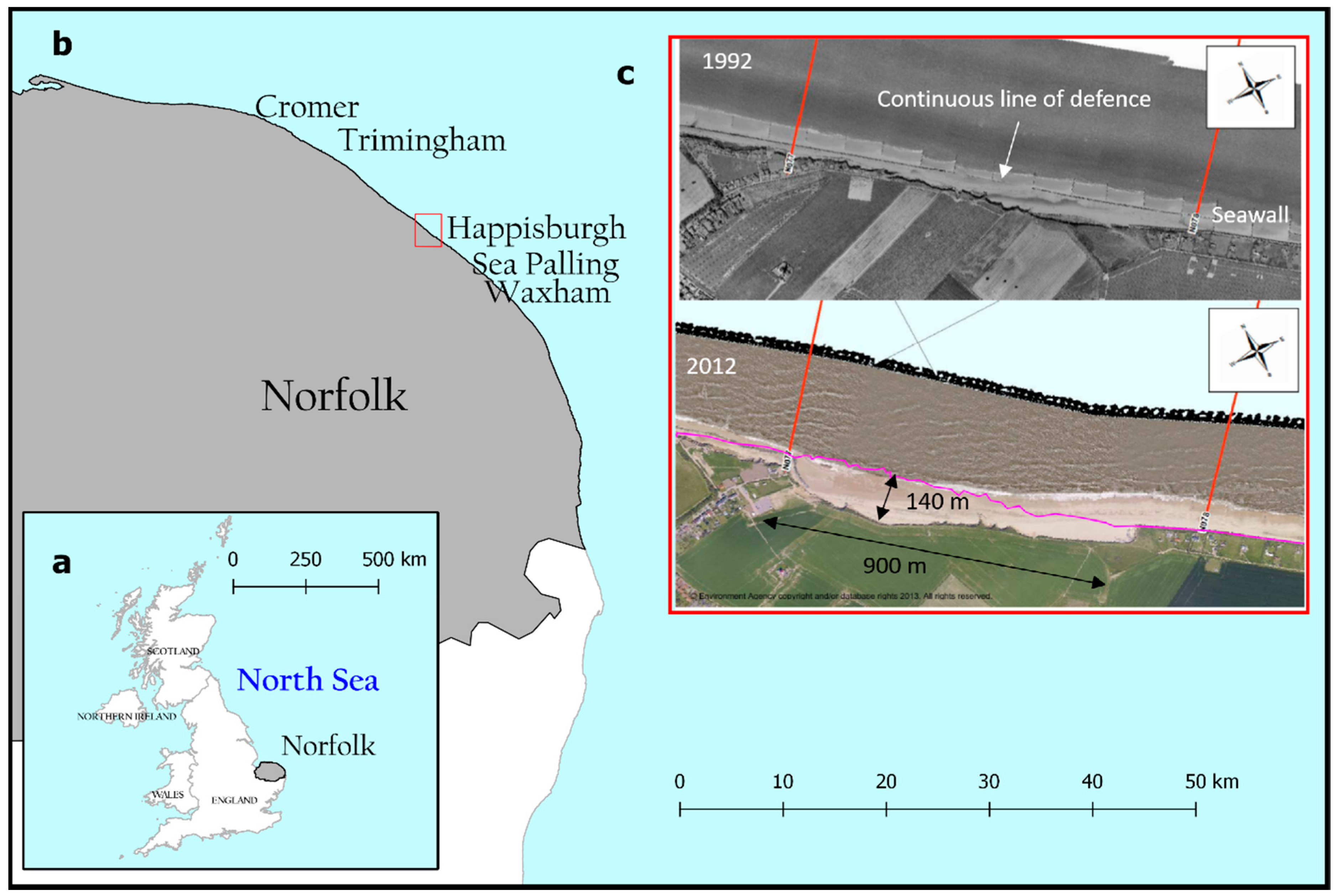
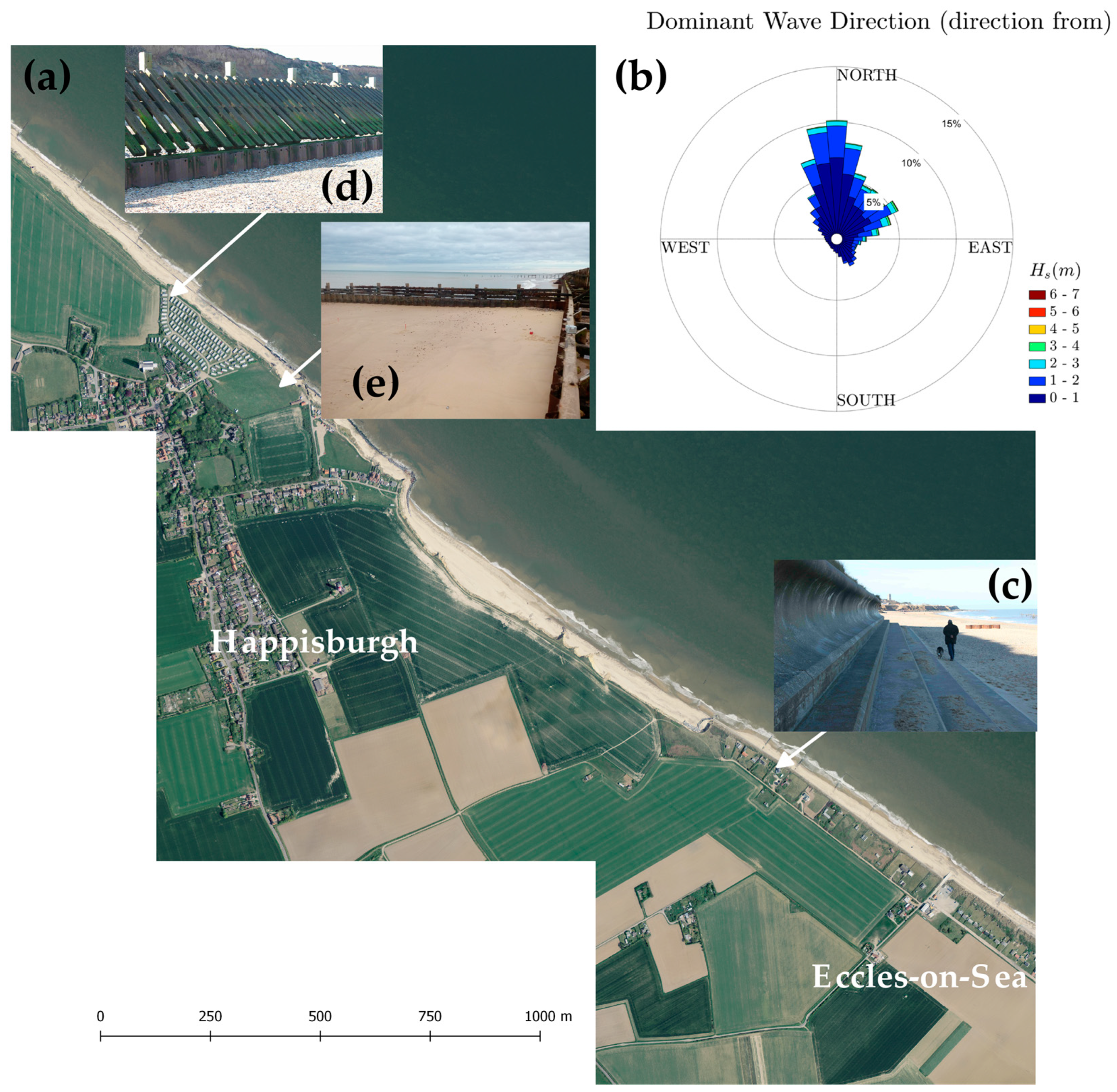
2. Study Site
3. Materials and Methods
3.1. Field Observations
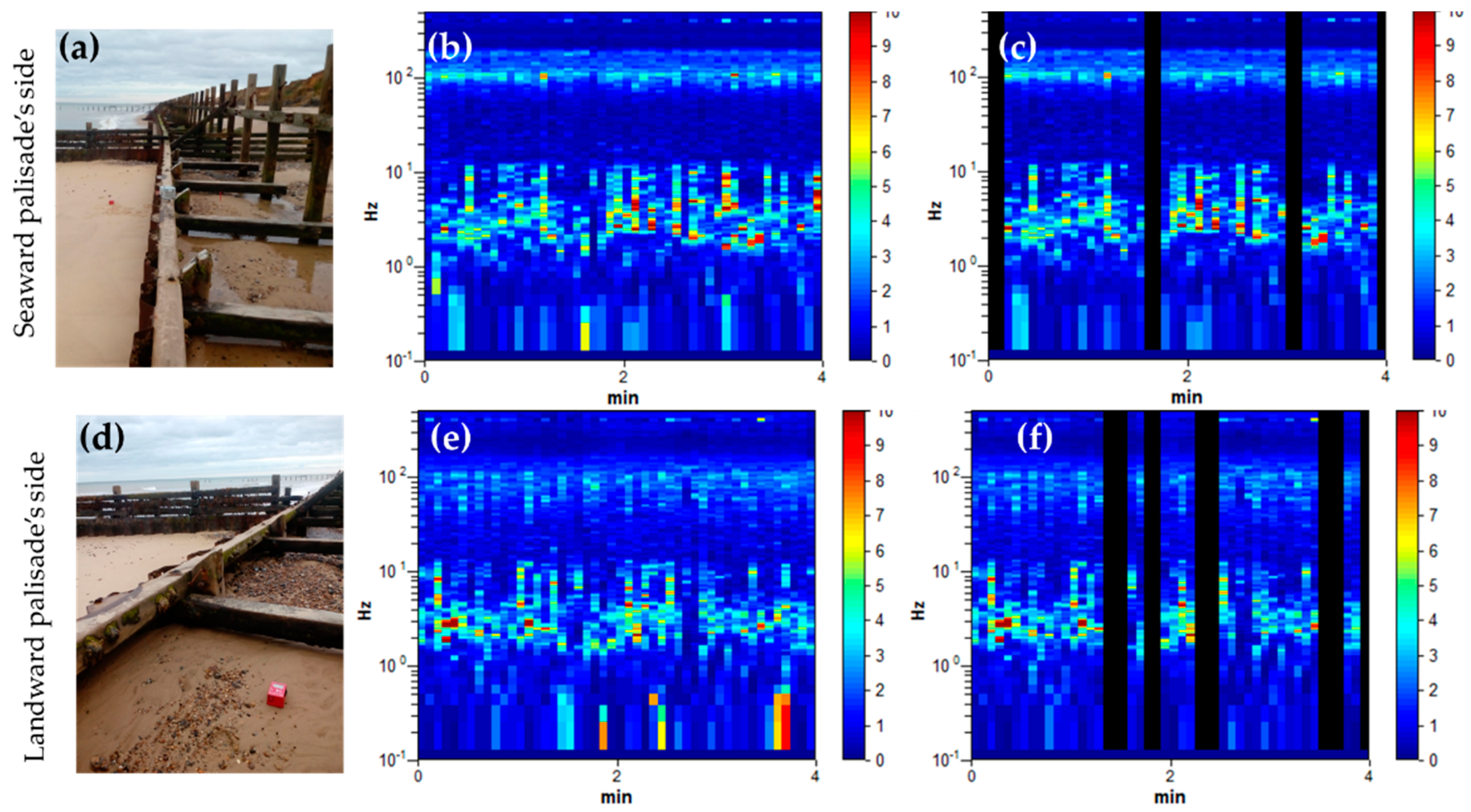
3.1.1. Passive Seismic Survey
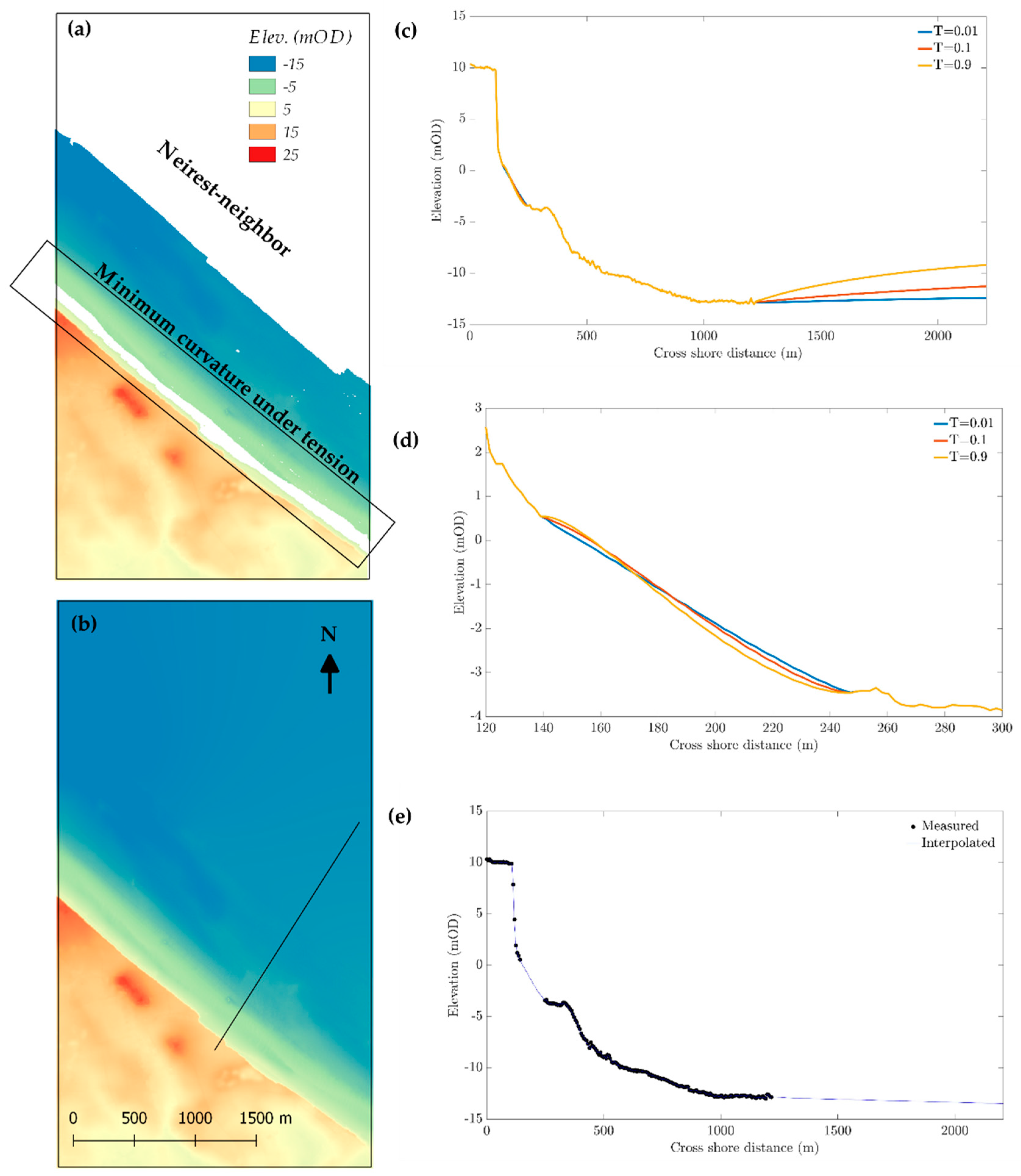
3.1.2. Digital Terrain Model of Study Area
3.2. Numerical Modelling
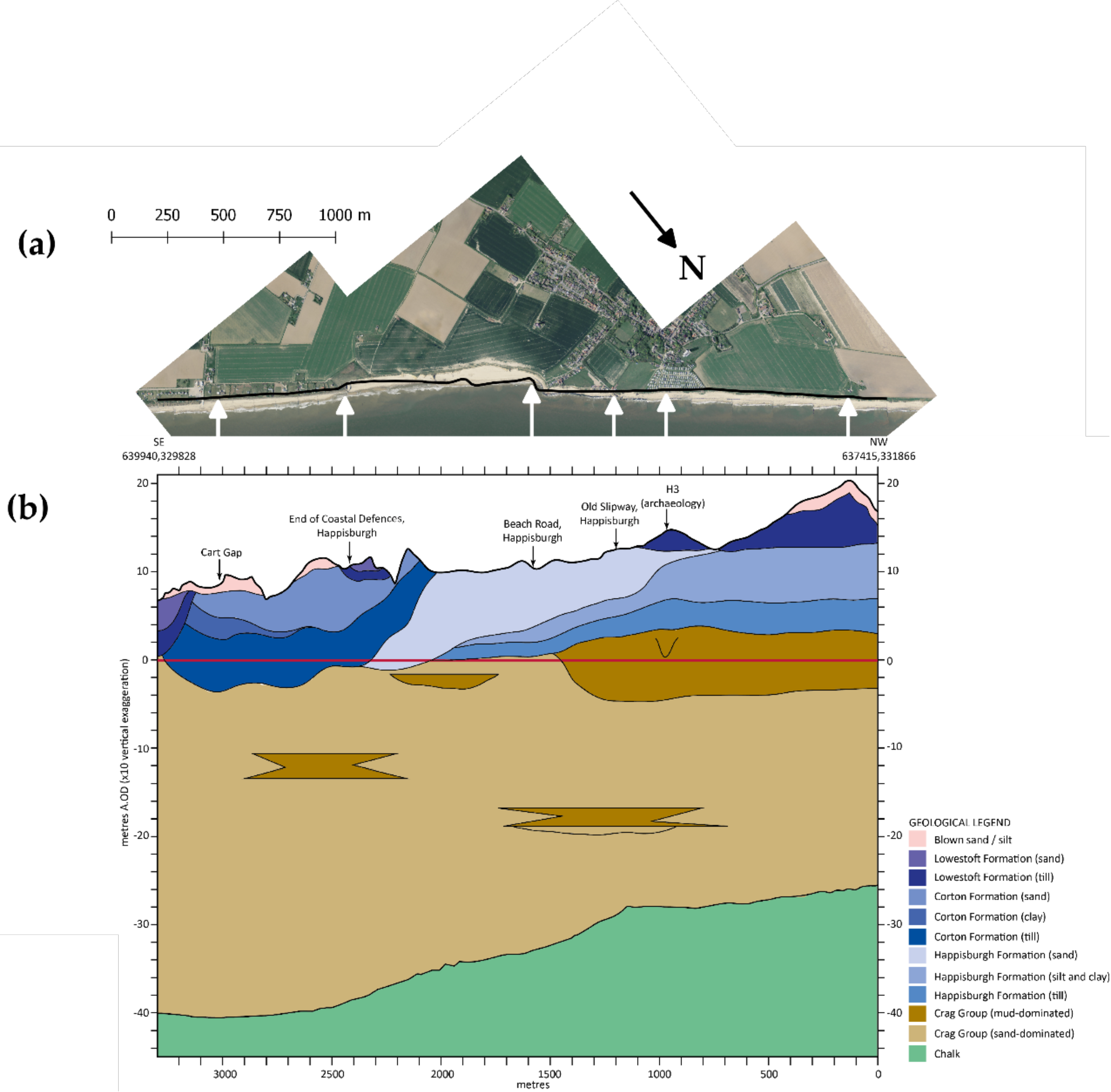
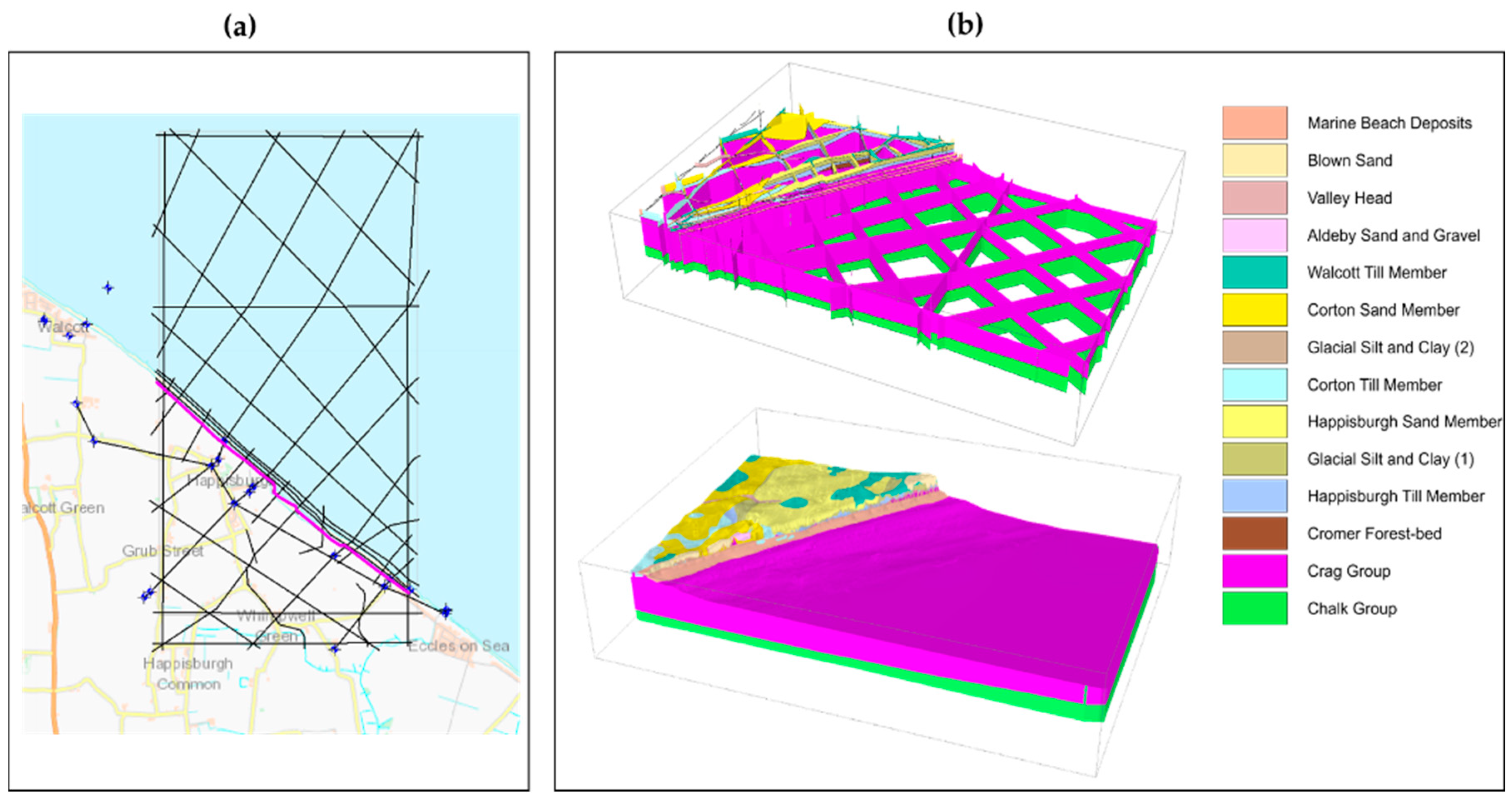
3.2.1. 3D Subsurface Model
3.2.2. Landscape Evolution Modelling: CoastalME
- Initialize the thickness model: The DTM and lithological model are converted into a raster thickness model that represent the ground elevation and the consolidated and non-consolidated stock of coarse, sand and fine material in the subsurface.
- Define the intervention type and its above–ground elevation: The existing coastal defences (i.e., palisade and sea wall) are digitized and represented in a raster file. Raster cells marked as an intervention type are assumed not to erode over time. In addition to the location, the intervention has an assigned above-ground elevation that allows the model framework to assess if it is submerged or not at different tidal phases.
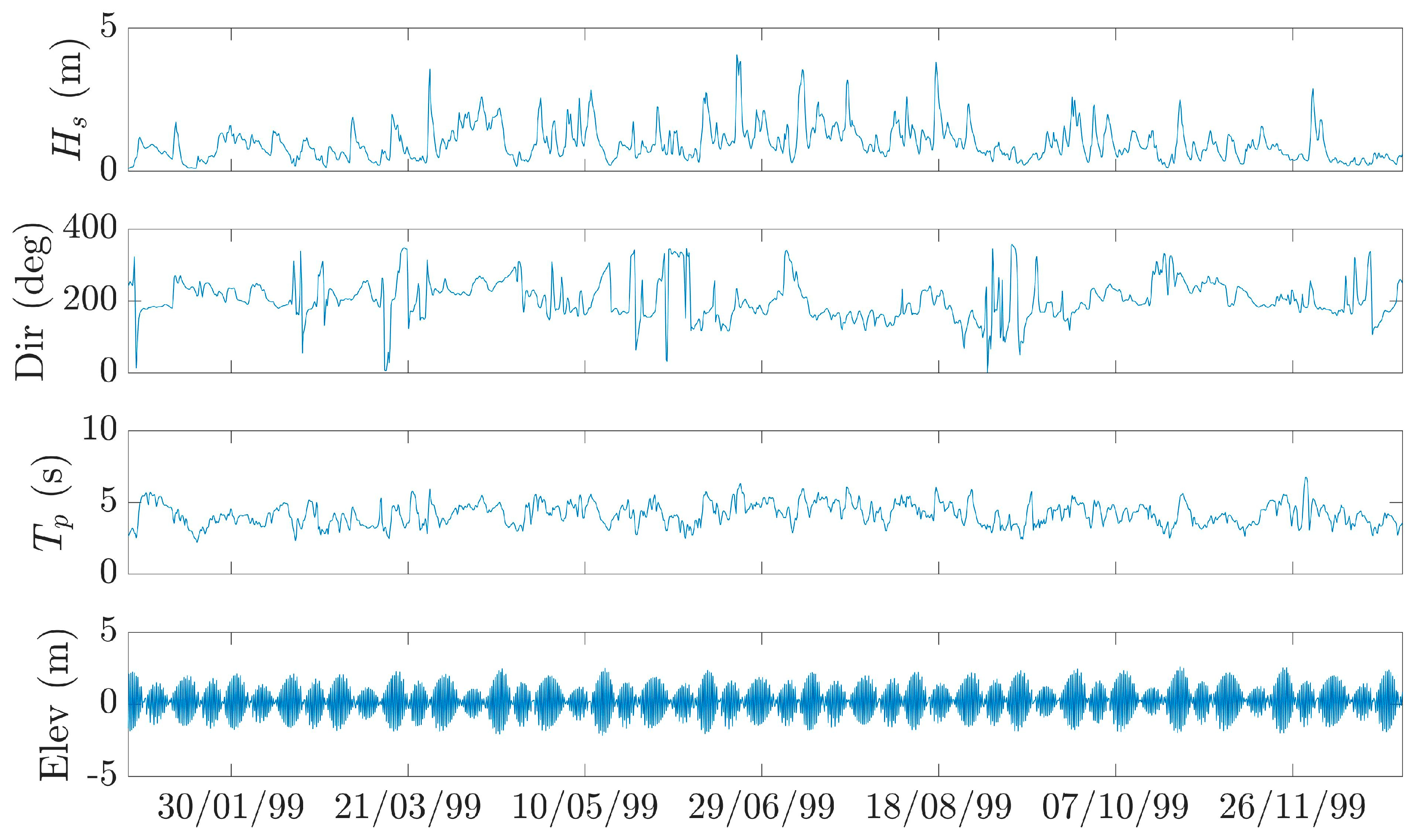
- Characterize the driving forces and resistance forces: for this exploratory assessment, we have assumed an idealized wave climate that represents the main drivers of coastal morphological change in the area. In particular, we have assumed a constant wave height, wave period and wave direction that roughly correspond with the net annual energy flux and we vary the tide level every hour according to the tidal harmonics registered at the nearby tide station in Cromer. The resistance cliff downwearing has been assumed equal to the cliff back wearing resistance and was calibrated to reproduce the observed cliff erosion between 1999 and 2004.
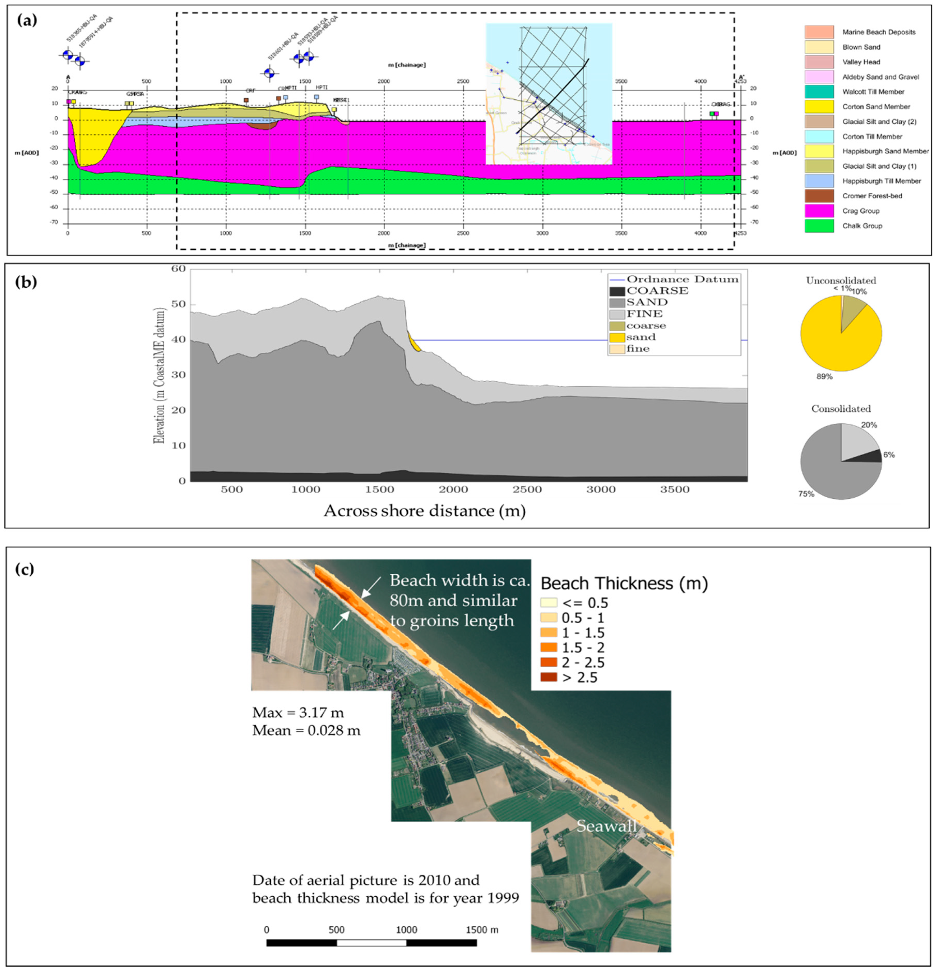
3.2.3. Converting 3D Lithological Model into CoastalME Thickness Model
4. Results
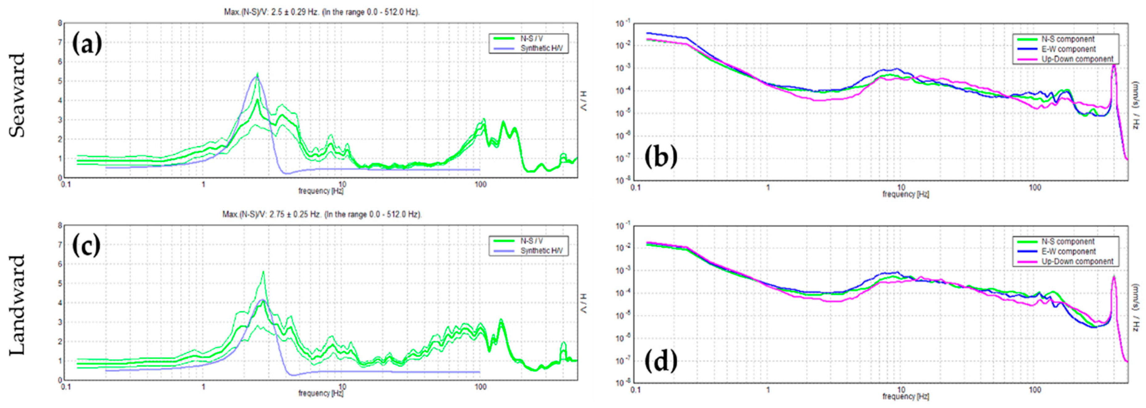
4.1. Passive Seismic Survey Results in Front and behind the Defences
4.2. Beach Thickness Along-Shore Variability at Happisburgh
4.3. Landscape Evolution Model Results
4.3.1. Model Calibration and Validation
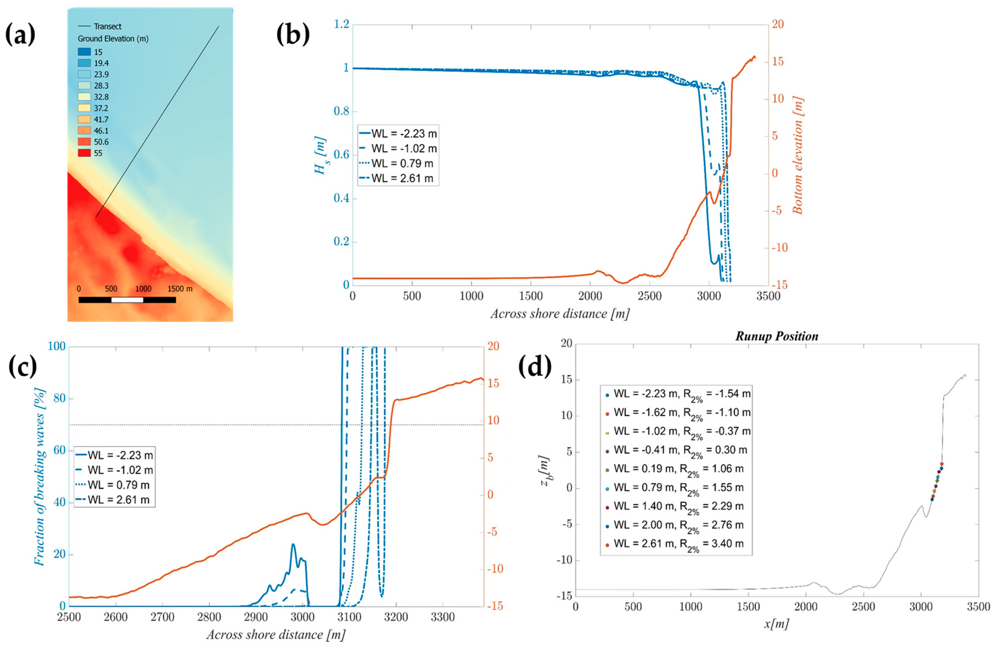
4.3.2. Wave Breaking and Wave Run-Up over a Full Tidal Cycle
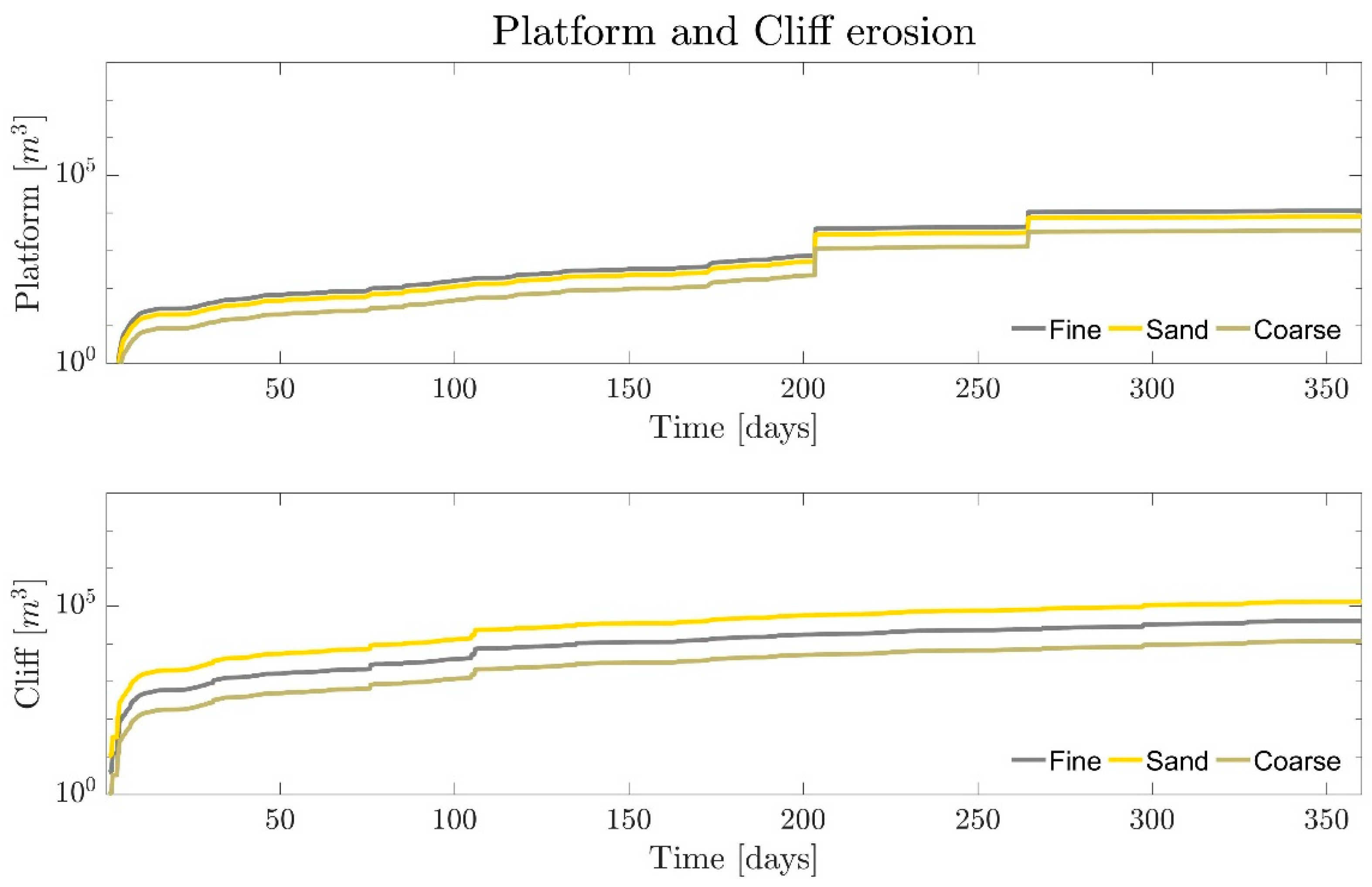
4.3.3. Daily Simulated Volumetric Changes
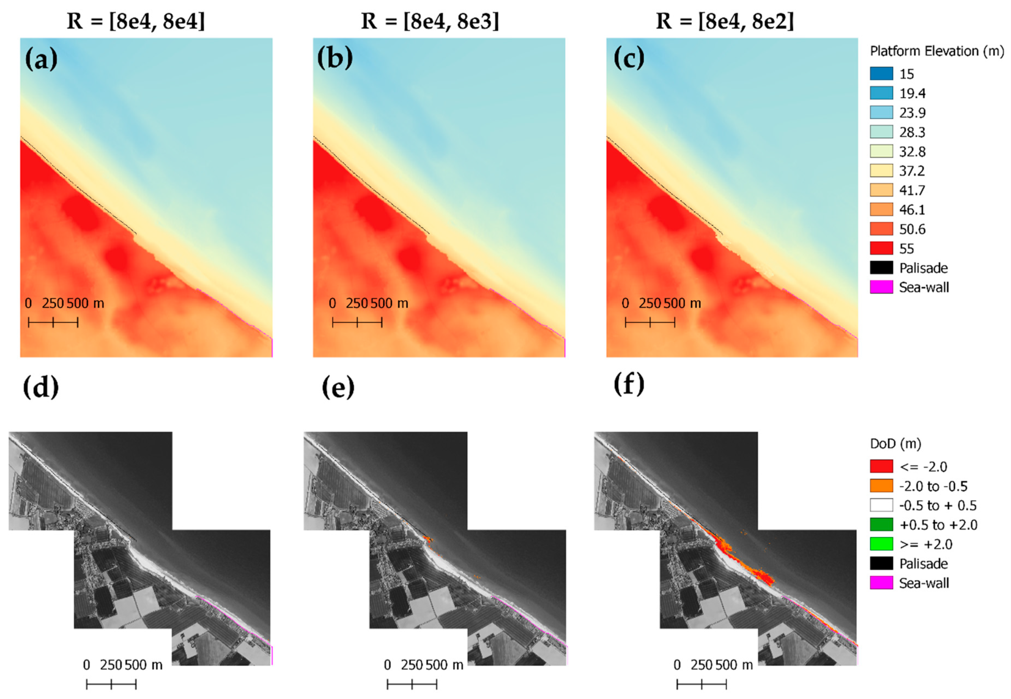
4.3.4. Digital Elevation Model of Topographic and Thickness Difference
5. Discussion
5.1. Happisburgh Beach Conceptualized as a Thin but Non-Sediment Starving Beach
5.2. Contribution of Platform Back-Wearing and Down-Wearing to Near-Shore Sediment Budgets
5.3. Implications and Limitations
6. Conclusions
Supplementary Materials
Author Contributions
Funding
Acknowledgments
Conflicts of Interest
Appendix A. Criteria for Reliable and Clear H/V

| Max. H/V at 2.5 ± 54.26 Hz (in the Range 0.0–512.0 Hz). | |||
|---|---|---|---|
| Criteria for a reliable H/V curve [All 3 should be fulfilled] | |||
| f0 > 10/Lw | 2.50 > 2.00 | OK | |
| nc(f0) > 200 | 512.5 > 200 | OK | |
| sA(f) < 2 for 0.5f0 < f < 2f0 if f0 > 0.5Hz | Exceeded 0 out of 31 times | OK | |
| sA(f) < 3 for 0.5f0 < f < 2f0 if f0 < 0.5Hz | |||
| Criteria for a clear H/V peak [At least 5 out of 6 should be fulfilled] | |||
| Exists f− in [f0/4, f0] | AH/V(f−) < A0/2 | 1.5 Hz | OK | |
| Exists f+ in [f0, 4f0] | AH/V(f+) < A0/2 | 5.5 Hz | OK | |
| A0 > 2 | 4.20 > 2 | OK | |
| fpeak[AH/V(f) ± sA(f)] = f0 ± 5% | |21.70298| < 0.05 | NO | |
| sf < e(f0) | 54.25745 < 0.125 | NO | |
| sA(f0) < q(f0) | 1.2164 < 1.58 | OK | |
| Threshold Values for sf and sA(f0) | |||||
|---|---|---|---|---|---|
| Freq. range [Hz] | <0.2 | 0.2–0.5 | 0.5–1.0 | 1.0–2.0 | >2.0 |
| e(f0) [Hz] | 0.25 f0 | 0.2 f0 | 0.15 f0 | 0.10 f0 | 0.05 f0 |
| q(f0) for sA(f0) | 3.0 | 2.5 | 2.0 | 1.78 | 1.58 |
| log q(f0) for slogH/V(f0) | 0.48 | 0.40 | 0.30 | 0.25 | 0.20 |
| Max. H/V at 2.75 ± 0.92 Hz (in the Range 0.0–512.0 Hz). | |||
|---|---|---|---|
| Criteria for a reliable H/V curve [All 3 should be fulfilled] | |||
| f0 > 10/Lw | 2.75 > 2.00 | OK | |
| nc(f0) > 200 | 495.0 > 200 | OK | |
| sA(f) < 2 for 0.5f0 < f < 2f0 if f0 > 0.5Hz | Exceeded 0 out of 34 times | OK | |
| sA(f) < 3 for 0.5f0 < f < 2f0 if f0 < 0.5Hz | |||
| Criteria for a clear H/V peak [At least 5 out of 6 should be fulfilled] | |||
| Exists f− in [f0/4, f0] | AH/V(f −) < A0/2 | 1.5 Hz | OK | |
| Exists f+ in [f0, 4f0] | AH/V(f +) < A0/2 | 5.125 Hz | OK | |
| A0 > 2 | 3.98 > 2 | OK | |
| fpeak[AH/V(f) ± sA(f)] = f0 ± 5% | |0.33445| < 0.05 | NO | |
| sf < e(f0) | 0.91974 < 0.1375 | NO | |
| sA(f0) < q(f0) | 1.2647 < 1.58 | OK | |
| Lw | window length |
| nw | number of windows used in the analysis |
| nc = Lw nw f0 | number of significant cycles |
| f | current frequency |
| f0 | H/V peak frequency |
| sf | standard deviation of H/V peak frequency |
| e(f0) | threshold value for the stability condition sf < e(f0) |
| A0 | H/V peak amplitude at frequency f0 |
| AH/V(f) | H/V curve amplitude at frequency f |
| f− | frequency between f0/4 and f0 for which AH/V(f−) < A0/2 |
| f+ | frequency between f0 and 4f0 for which AH/V(f+) < A0/ |
| sA(f) | standard deviation of AH/V(f), sA(f) is the factor by which the mean AH/V(f) curve should be multiplied or divided |
| slogH/V(f) | standard deviation of log AH/V(f) curve |
| q(f0) | threshold value for the stability condition sA(f) < q(f0) |
| Threshold Values for sf and sA(f0) | |||||
|---|---|---|---|---|---|
| Freq. range [Hz] | <0.2 | 0.2–0.5 | 0.5–1.0 | 1.0–2.0 | >2.0 |
| e(f0) [Hz] | 0.25 f0 | 0.2 f0 | 0.15 f0 | 0.10 f0 | 0.05 f0 |
| q(f0) for sA(f0) | 3.0 | 2.5 | 2.0 | 1.78 | 1.58 |
| log q(f0) for slogH/V(f0) | 0.48 | 0.40 | 0.30 | 0.25 | 0.20 |
Appendix B. Supplementary Lithological, Hydrodynamic and Morphodynamic Information
| Name | Lithology | Coarse [%] | Sand [%] | Fine [%] |
|---|---|---|---|---|
| Marine beach deposits | Shoreline sand and gravel | 10 | 89 | 1 |
| Coastal barrier deposits | sand and gravel | 10 | 89 | 1 |
| Breydon Formation | Holocene peat, silt, clay. Tidal alluvium | 2 | 30 | 68 |
| Blown sand | wind blown sand | 0.5 | 84.5 | 15 |
| Valley head | clay, silt, sand, gravel | 10 | 35 | 55 |
| Aldeby Sand and Gravel | Sand and gravel overlying chalky till | 10 | 83 | 7 |
| Walcott Till Member | Very chalky till, up to 70 per cent | 15 | 7.5 | 77.5 |
| Corton Sand Member | sand, with some gravel | 5 | 85 | 10 |
| Glacial silt and clay | laminated silt and clay (mud) | 0.5 | 10 | 89.5 |
| Corton Till Member | Sandy, silty diamicton (aka brickearth) | 10 | 35 | 55 |
| Happisburgh Sand Member | Sand | 2 | 90 | 8 |
| Glacial silt and clay | laminated silt and clay (mud) | 0.5 | 10 | 89.5 |
| Happisburgh Till Member | Sandy, silty diamicton | 10 | 35 | 55 |
| Cromer Forest-bed | mud | 10 | 30 | 60 |
| Crag Group | sand | 5 | 85 | 10 |
| chalk | chalk | 15 | 2 | 83 |

| Water Level (m) | Hs at z = 0 (m) | 2% Run Up |
|---|---|---|
| −2.23 | 0.13 | −1.54 |
| −1.62 | 0.16 | −1.10 |
| −1.02 | 0.16 | −0.37 |
| −0.41 | 0.23 | 0.30 |
| 0.19 | 0.19 | 1.06 |
| 0.79 | 0.20 | 1.55 |
| 1.40 | 0.24 | 2.29 |
| 2.00 | 0.28 | 2.76 |
| 2.61 | 0.10 | 3.40 |

References
- Pontee, N.I.; Parsons, A. A review of coastal risk management in the UK. Proc. Inst. Civ. Eng.-Marit. Eng. 2010, 163, 31–42. [Google Scholar] [CrossRef]
- Dickson, M.E.; Walkden, M.J.A.; Hall, J.W. Systemic impacts of climate change on an eroding coastal region over the twenty-first century. Clim. Chang. 2007, 84, 141–166. [Google Scholar] [CrossRef]
- Walkden, M.; Watson, G.; Johnson, A.; Heron, E.; Tarrant, O. Coastal catch-up following defence removal at Happisburgh. In Coastal Management; ICE Publishing: London, UK, 2016; pp. 523–532. [Google Scholar]
- Payo, A.; Walkden, M.; Barkwith, A.; Ellis, A.M. Modelling rapid coastal catch-up after defence removal along the soft cliff coast of Happisburgh, UK. In Proceedings of the 36th International Conference on Coastal Engineering, Baltimore, MD, USA, 30 July–3 August 2018; ASCE: Baltimore, MD, USA; p. 2. [Google Scholar]
- Shennan, I.; Woodworth, P.L. A comparison of late holocene and twentieth-century sea-level trends from the UK and North Sea region. Geophys. J. Int. 1992, 109, 96–105. [Google Scholar] [CrossRef]
- Hayman, S. Eccles to Winterton on Sea Coastal Defences; SH/RG BF190712; Environment Agency: Bristol, UK, 2012; p. 3. [Google Scholar]
- Wolf, J.; Lowe, J.; Howard, T. Climate downscaling: Local mean sea level, surge and wave modelling. In Broad Scale Coastal Simulation; Springer: Berlin, Germany, 2015; pp. 79–102. [Google Scholar]
- Geos, F. Wind and Wave Frequency Distributions for Sites around the British Isles; Health and Safety Executive: Bootle, UK, 2001. [Google Scholar]
- Brown, S.; Barton, M.E.; Nicholls, R.J. Shoreline response of eroding soft cliffs due to hard defences. Proc. ICE-Marit. Eng. 2014, 167, 3–14. [Google Scholar]
- Clayton, K.M. Sediment input from the norfolk cliffs, eastern england—A century of coast protection and its effect. J. Coast. Res. 1989, 5, 433–442. [Google Scholar]
- Poulton, C.V.; Lee, J.; Hobbs, P.; Jones, L.; Hall, M. Preliminary investigation into monitoring coastal erosion using terrestrial laser scanning: Case study at Happisburgh, Norfolk. Bull. Geol. Soc. Norfolk 2006, 56, 45–64. [Google Scholar]
- Frew, P. Adapting to coastal change in north Norfolk, UK. Proc. Inst. Civ. Eng.-Marit. Eng. 2012, 165, 131–138. [Google Scholar] [CrossRef]
- Lunkka, J.P. Sedimentation and iithostratigraphy of the north sea drift and lowestoft till formations in the coastal cliffs of northeast Norfolk, England. J. Quat. Sci. 1994, 9, 209–233. [Google Scholar] [CrossRef]
- Lee, J.R. Early and Middle Pleistocene Lithostratigraphy and Palaeo-Environments in Northern East Anglia; Royal Holloway, University of London: London, UK, 2003. [Google Scholar]
- Lee, J.R.; Phillips, E.R. Progressive soft sediment deformation within a subglacial shear zone—A hybrid mosaic-pervasive deformation model for middle pleistocene glaciotectonised sediments from eastern England. Quat. Sci. Rev. 2008, 27, 1350–1362. [Google Scholar] [CrossRef]
- Lee, J.R.; Phillips, E.; Rose, J.; Vaughan-Hirsch, D. The middle pleistocene glacial evolution of northern East Anglia, UK: A dynamic tectonostratigraphic–parasequence approach. J. Quat. Sci. 2017, 32, 231–260. [Google Scholar] [CrossRef]
- Parfitt, S.A.; Ashton, N.M.; Lewis, S.G.; Abel, R.L.; Coope, G.R.; Field, M.H.; Gale, R.; Hoare, P.G.; Larkin, N.R.; Lewis, M.D. Early pleistocene human occupation at the edge of the boreal zone in northwest europe. Nature 2010, 466, 229–233. [Google Scholar] [CrossRef] [PubMed]
- West, R.G. The Pre-Glacial Pleistocene of the Norfolk and Suffolk Coasts. Archeol. J. 1981, 138, 266–267. [Google Scholar]
- Aki, K.; Richards, P.G. Quantitative Seismology; University Science Books: Sausalito, CA, USA, 2002. [Google Scholar]
- Ari, B.-M.; Singh, S.J. Seismic Waves and Sources; Springer: New York, NY, USA, 1981. [Google Scholar]
- Guillier, B.; Chatelain, J.-L.; Bonnefoy-Claudet, S.; Haghshenas, E. Use of ambient noise: From spectral amplitude variability to H/V stability. J. Earthq. Eng. 2007, 11, 925–942. [Google Scholar] [CrossRef]
- SESAME. Guidelines for the Implementation of the H/V Spectral Ratio Technique on Ambient Vibrations-Measurements, Processing and Interpretation; Sesame European Research Project, Deliverable d23. 12., Project No; EVG1-CT-2000-00026 SESAME, 62; 2004; Available online: http://www.geopsy.org/ (accessed on 4 October 2018).
- Bonnefoy-Claudet, S.; Köhler, A.; Cornou, C.; Wathelet, M.; Bard, P.Y. Effects of love waves on microtremor h/v ratio. Bull. Seismol. Soc. Am. 2008, 98, 288–300. [Google Scholar] [CrossRef]
- Conrad, O.; Bechtel, B.; Bock, M.; Dietrich, H.; Fischer, E.; Gerlitz, L.; Wehberg, J.; Wichmann, V.; Böhner, J. System for automated geoscientific analyses (saga) v. 2.1.4. Geosci. Model Dev. 2015, 8, 1991–2007. [Google Scholar] [CrossRef]
- Smith, W.; Wessel, P. Gridding with continuous curvature splines in tension. Geophysics 1990, 55, 293–305. [Google Scholar] [CrossRef]
- Kessler, H.; Mathers, S.; Sobisch, H.-G. The capture and dissemination of integrated 3d geospatial knowledge at the british geological survey using gsi3d software and methodology. Comput. Geosci. 2009, 35, 1311–1321. [Google Scholar] [CrossRef]
- Payo, A.; Favis-Mortlock, D.; Dickson, M.; Hall, J.W.; Hurst, M.; Walkden, M.J.A.; Townend, I.; Ives, M.C.; Nicholls, R.J.; Ellis, M.A. Coastalme version 1.0: A coastal modelling environment for simulating decadal to centennial morphological changes. Geosci. Model Dev. Discuss. 2016, 2016, 1–45. [Google Scholar] [CrossRef]
- Payo, A.; Favis-Mortlock, D.; Dickson, M.; Hall, J.W.; Hurst, M.D.; Walkden, M.J.A.; Townend, I.; Ives, M.C.; Nicholls, R.J.; Ellis, M.A. Coastal modelling environment version 1.0: A framework for integrating landform-specific component models in order to simulate decadal to centennial morphological changes on complex coasts. Geosci. Model Dev. 2017, 10, 2715–2740. [Google Scholar] [CrossRef]
- Hurst, M.D.; Barkwith, A.; Ellis, M.A.; Thomas, C.W.; Murray, A.B. Exploring the sensitivities of crenulate bay shorelines to wave climates using a new vector-based one-line model. J. Geophys. Res. Earth Surf. 2015, 120, 2586–2608. [Google Scholar] [CrossRef]
- Kobayashi, N. Coastal sediment transport modeling for engineering applications. J. Waterw. Port Coast. Ocean Eng. 2016, 142, 03116001. [Google Scholar] [CrossRef]
- Walkden, M.; Dickson, M.; Thomas, J.; Hall, J. Probabilistic Simulation of Long Term Shore Morphology of North Norfolk UK; World Scientific: Singapore, 2009; pp. 4365–4377. [Google Scholar]
- Walkden, M.J.; Hall, J.W. A mesoscale predictive model of the evolution and management of a soft-rock coast. J. Coast. Res. 2011, 27, 529–543. [Google Scholar] [CrossRef]
- Self, S.; Entwisle, D.; Northmore, K. The Structure and Operation of the BGS National Geotechnical Properties Database; Version 2; British Geological Survey: Nottingham, UK, 2012. [Google Scholar]
- Ohl, C.; Frew, P.; Sawyers, P.; Watson, G.; Lawton, P.; Farrow, B.; Walkden, M.; Hall, J. North Norfolk—A regional approach to coastal erosion management and sustainability in practice. In Proceedings of the International Conference on Coastal ManagementInstitution of Civil Engineers 2003, Brighton, UK, 15–17 October 2003. [Google Scholar]
- Codiga, D.L. Unified Tidal Analysis and Prediction Using the Utide Matlab Functions; Graduate School of Oceanography, University of Rhode Island: Narragansett, RI, USA, 2011. [Google Scholar]
- Le Hir, P.; Cayocca, F.; Waeles, B. Dynamics of sand and mud mixtures: A multiprocess-based modelling strategy. Cont. Shelf Res. 2011, 31, S135–S149. [Google Scholar] [CrossRef]
- Walkden, M.J.A.; Hall, J.W. A predictive mesoscale model of the erosion and profile development of soft rock shores. Coast. Eng. 2005, 52, 535–563. [Google Scholar] [CrossRef]
- Cambers, G. Temporal scales in coastal erosion systems. Trans. Inst. Br. Geogr. 1976, 1, 246–256. [Google Scholar] [CrossRef]


| Model | Method | Implementation in CoastalME |
|---|---|---|
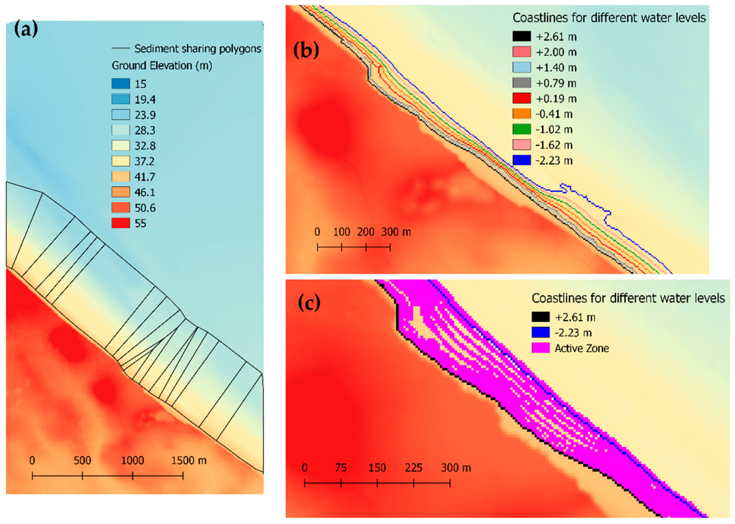
| COVE | ‘one-line’ model designed to handle complex coastline geometries, with high platform curvature shorelines [29] | CoastalME as COVE, uses a local coordinate scheme (rather than global), and divide the coastline as a set of sediment sharing polygonal shapes (e.g., triangles and trapezoids). For each polygon, the potential alongshore sediment is calculated using CERC equation using polygon averaged breaking wave and sediment size properties. Actual alongshore sediment transport is constrained by unconsolidated sediment availability. |
| CSHORE | One-dimensional time-averaged near-shore profile model for predictions of wave height, water level, wave-induced steady currents, and beach profile evolution and stone structural damage progression [30]. | CoastalME propagates the wave properties by calling CSHORE hydrodynamic module along a number of cross-shore profiles. Wave properties between profiles are interpolated to provide polygon averaged values. |
| SCAPE | One line model which includes the beach and platform interactions. Its principal modules describe wave transformation, platform erosion, and a (one-line) beach [31,32]. | CostalME simulates beach and platform erosion as in SCAPE. The original horizontal SCAPE erosion is converted into its vertical component by applying a simple trigonometrical conversion (Equation (6) in [28]). |
| Input | Value |
|---|---|
| Required for a generic landscape evolution model | |
| Run duration | 360 days |
| Time step | 6 h |
| Wave heights, direction, period | UKCP09 hindcast data |
| Topo and bathymetric Digital Elevation Model | LiDAR year 1999 & Multibeam 2011 |
| Tides | Reconstruction of tidal signal using Cromer tide gauge data from 1999 to 2017 |
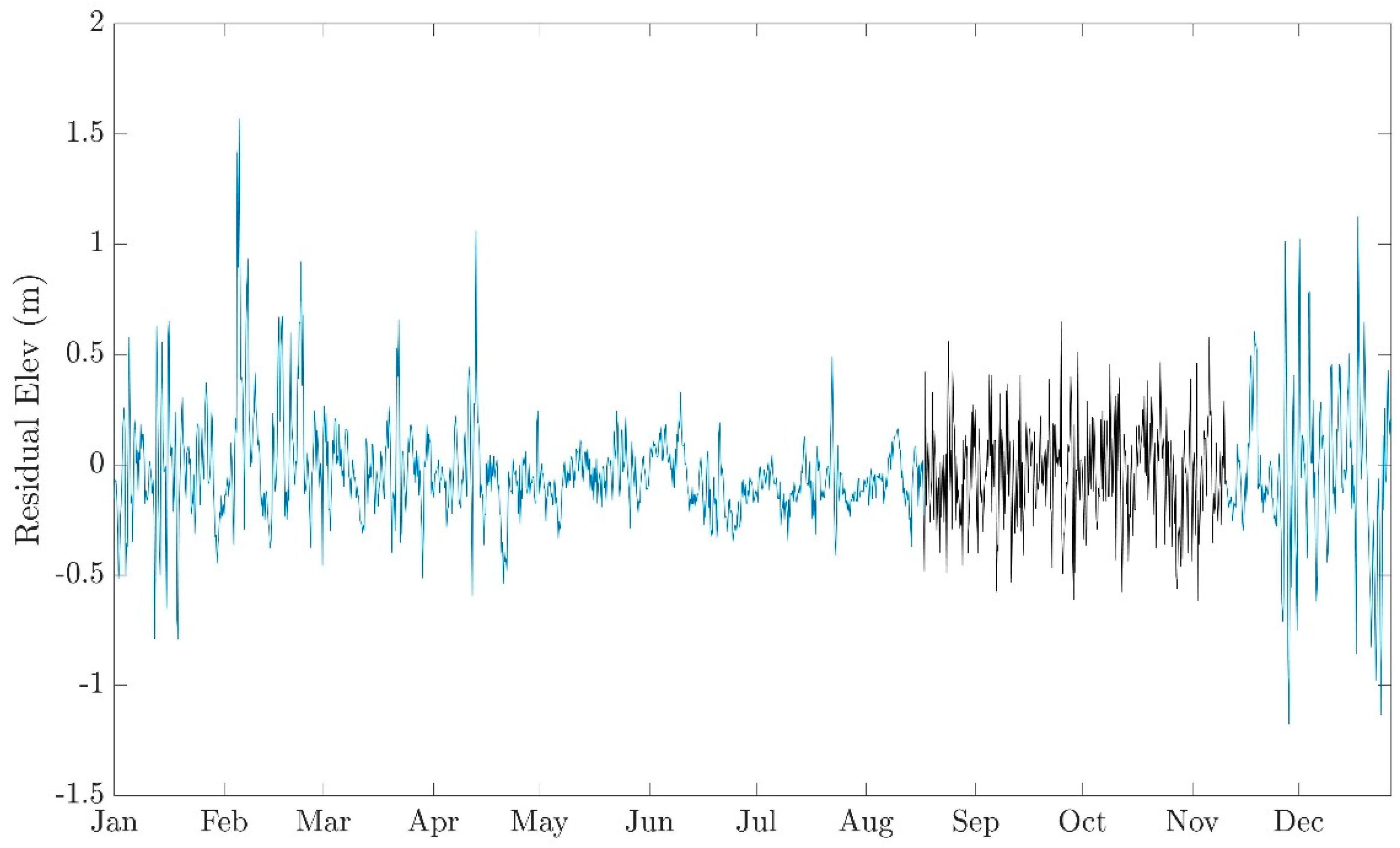
| Residual elevation | Difference of Cromer tide gauge elevation and tidal levels (gap filled assuming residuals follow a normal distribution) |
| CoastalME Datum | +40 m above basement level |
| Coarse, sand and fine sediment content | BGS thickness model |
| Coarse, sand and fine availability factor | 0.3; 0.7; 1.0 |
| Boundary conditions | Open boundaries (i.e., sediment at the boundaries is allotted to exit the grid but no external sediment inputs are assumed over the simulated period) |
| Required for COVE-sediment sharing module | |
| CERC coefficient | 0.79 |
| Length of normal profiles used to create the polygons | 800 m |
| Required for CSHORE-wave propagation module | |
| Breaker ratio parameter γ | 0.8 |
| Friction factor fb | 0.015 |
| Required for SCAPE-beach & platform interaction | |
| Rock strength and hydrodynamic constant, R | RPlatform = 8 × 10⁴ [m9/4s2/3] RCliff = 8 × 10² [m9/4s2/3] |
| Beach volume & and beach thickness | Derived from BGS thickness model |
| Full list of parameters provided in Table S1 | |
| Platform Erosion |
| Total potential platform erosion = 25,612.27 m3 |
| Total actual platform erosion = 22,584.25 m3 |
| Total fine actual platform erosion = 11,292.12 m3 |
| Total sand actual platform erosion = 7904.49 m3 |
| Total coarse actual platform erosion = 3387.64 m3 |
| Cliff Collapse |
| Total cliff collapse = 181,708.20 m3 |
| Total fine cliff collapse = 40,646.87 m3 |
| Total sand cliff collapse = 129,436.91 m3 |
| Total coarse cliff collapse = 11,624.42 m3 |
| Beach Erosion |
| Total potential beach erosion = 88,958.33 m3 |
| Total actual beach erosion = 6244.53 m3 |
| Total actual fine beach erosion = 133.40 m3 |
| Total actual sand beach erosion = 4774.00 m3 |
| Total actual coarse beach erosion = 1337.13 m3 |
| Beach Deposition |
| Total beach deposition = 17,376.80 m3 |
| Total sand beach deposition = 12,660.11 m3 |
| Total coarse beach deposition = 4716.69 m3 |
| Suspended Sediment |
| Suspended fine sediment = 1415.153 m3 |
| Simulation results for model setup as shown in Table 2 |
| Initial (m3) | Change (m3) | |
|---|---|---|
| Total | 392.559,461 | −252,343 |
| Beach (un consolidated) | 342,622 | −112,419 |
| Platform (consolidated) | 392,256.014 | −179,099 |
| Suspended sediment | 0 | +52,072 |
| Simulation results for model setup shown in Table 2 | ||
© 2018 by the authors. Licensee MDPI, Basel, Switzerland. This article is an open access article distributed under the terms and conditions of the Creative Commons Attribution (CC BY) license (http://creativecommons.org/licenses/by/4.0/).
Share and Cite
Payo, A.; Walkden, M.; Ellis, M.A.; Barkwith, A.; Favis-Mortlock, D.; Kessler, H.; Wood, B.; Burke, H.; Lee, J. A Quantitative Assessment of the Annual Contribution of Platform Downwearing to Beach Sediment Budget: Happisburgh, England, UK. J. Mar. Sci. Eng. 2018, 6, 113. https://doi.org/10.3390/jmse6040113
Payo A, Walkden M, Ellis MA, Barkwith A, Favis-Mortlock D, Kessler H, Wood B, Burke H, Lee J. A Quantitative Assessment of the Annual Contribution of Platform Downwearing to Beach Sediment Budget: Happisburgh, England, UK. Journal of Marine Science and Engineering. 2018; 6(4):113. https://doi.org/10.3390/jmse6040113
Chicago/Turabian StylePayo, Andres, Mike Walkden, Michael A. Ellis, Andrew Barkwith, David Favis-Mortlock, Holger Kessler, Benjamin Wood, Helen Burke, and Jonathan Lee. 2018. "A Quantitative Assessment of the Annual Contribution of Platform Downwearing to Beach Sediment Budget: Happisburgh, England, UK" Journal of Marine Science and Engineering 6, no. 4: 113. https://doi.org/10.3390/jmse6040113
APA StylePayo, A., Walkden, M., Ellis, M. A., Barkwith, A., Favis-Mortlock, D., Kessler, H., Wood, B., Burke, H., & Lee, J. (2018). A Quantitative Assessment of the Annual Contribution of Platform Downwearing to Beach Sediment Budget: Happisburgh, England, UK. Journal of Marine Science and Engineering, 6(4), 113. https://doi.org/10.3390/jmse6040113