Regional Scale Risk-Informed Land-Use Planning Using Probabilistic Coastline Recession Modelling and Economical Optimisation: East Coast of Sri Lanka

Abstract

One of the measures that has been implemented widely to adapt to the effect of climate change in coastal zones is the implementation of set-back lines. The traditional approach of determining set-back lines is likely to be conservative, and thus pose unnecessary constraints on coastal zone development and fully utilising the potential of these high-return areas. In this study, we apply a newly developed risk-informed approach to determine the coastal set-back line at regional scale in a poor data environment. This approach aims to find the economic optimum by balancing the (potential) economic gain from investing in coastal zones and the risk of coastal retreat due to sea level rise and storm erosion. This application focusses on the east coast of Sri Lanka, which is experiencing rapid economic growth on one hand and severe beach erosion on the other hand. This area of Sri Lanka is a highly data-poor environment, and the data is mostly available from global databases and very limited measurement campaigns. Probabilistic estimates of coastline retreat are obtained from the application of Probabilistic Coastline Recession (PCR) framework. Economic data, such as the discount rate, rate of return of investment, cost of damage, etc., are collated from existing estimates/reports for the area. The main outcome of this study is a series of maps indicating the economically optimal set-back line (EOSL) for the ~200-km-long coastal region. The EOSL is established for the year 2025 to provide a stable basis for land-use planning decisions over the next two decades or so. The EOSLs thus determined range between 12 m and 175 m from the coastline. Sensitivity analyses show that strong variations in key economic parameters such as the discount rate have a disproportionately small impact on the EOSL.

1. Introduction

The effects of climate change on hydrodynamic forcing, such as sea level rise, changes in wave conditions, changes in the sediment supply from rivers, etc., is already resulting in changes in the rate of coastal erosion/accretion along the sandy coastlines of the world [1,2,3,4,5].

In light of climate change and especially coastline retreat due to sea level rise, many countries and coastal zone authorities are developing adaptation plans to protect coastal assets and future investments along their coastlines. These measures span a very wide range, from traditional hard structures, such as sea walls, and soft solutions such as (periodic) nourishment campaigns, to more modern strategies such as pre-storm interventions (coastal dune enforcements, transient breakwaters, etc.). One of the measures that has been widely implemented as part of the “accommodate” or “retreat” strategies in coastal zone management is the implementation of coastal set-back lines. A set-back line is a line along the coast, seaward of which certain development activities are prohibited or restricted. Traditionally, this line is determined based on a linear summation of long-term recession due to long-shore sediment transport gradients (estimated based on aerial photos or sediment budget modelling), the impact of storm erosion for a given return period (estimated from coastal profile modelling or historical data) and long-term recession due to sea level rise (estimated by the Bruun rule [6]). This method produces a set-back line that is likely to be conservative, resulting in rather severe constraints on coastal zone development. A risk-informed approach to coastal zone management was first proposed in 2002 [7], which was later refined [8,9]. The latter introduced the concept of the economically optimal set-back line (EOSL). This method, which balances the (potential) economic gain from coastal zone investments and the risk due to coastal erosion was applied to Narrabeen Beach, Sydney, Australia [9,10].

Two types of data are needed for determining the EOSL: economic data and probabilistic estimates of the development of coastline retreat in the future. Economic data, such as the discount rate, rate of return of investment (RoI), cost of damage, etc., may be collected from existing estimates/reports for the area of interest or be based on expert judgement. Probabilistic estimates of coastline retreat can be obtained from the Probabilistic Coastline Recession (PCR) framework [11]. The PCR framework is designed to perform Monte Carlo simulations, that is, to calculate a large number of long, realistic sequences of beach erosion and recovery, and to then statistically analyse the results instead of relying only on single storm effects with specific return period (i.e., deterministic estimates). Model inputs are statistical parameters representing the wave climate, water levels, and gaps between storms to randomly generate model boundary conditions. These parameters are derived using the Joint Probability Method (JPM), which considers not only a single event storm, but series of storm events [12,13]. This method includes allowances for joint probability between all basic erosion variates including: wave height, period and direction, event duration, and the time interval between events.

In this study, the above approach was applied along the east of Sri Lanka (Trincomalee and Batticaloa—Figure 1). The total study area spans over 200 km and in total 83 coastal profiles along the coastline were analysed. For each of the 83 profiles, the cumulative distribution function of probability of coastal retreat in the future was derived, which fed into the determination of the associated EOSL.

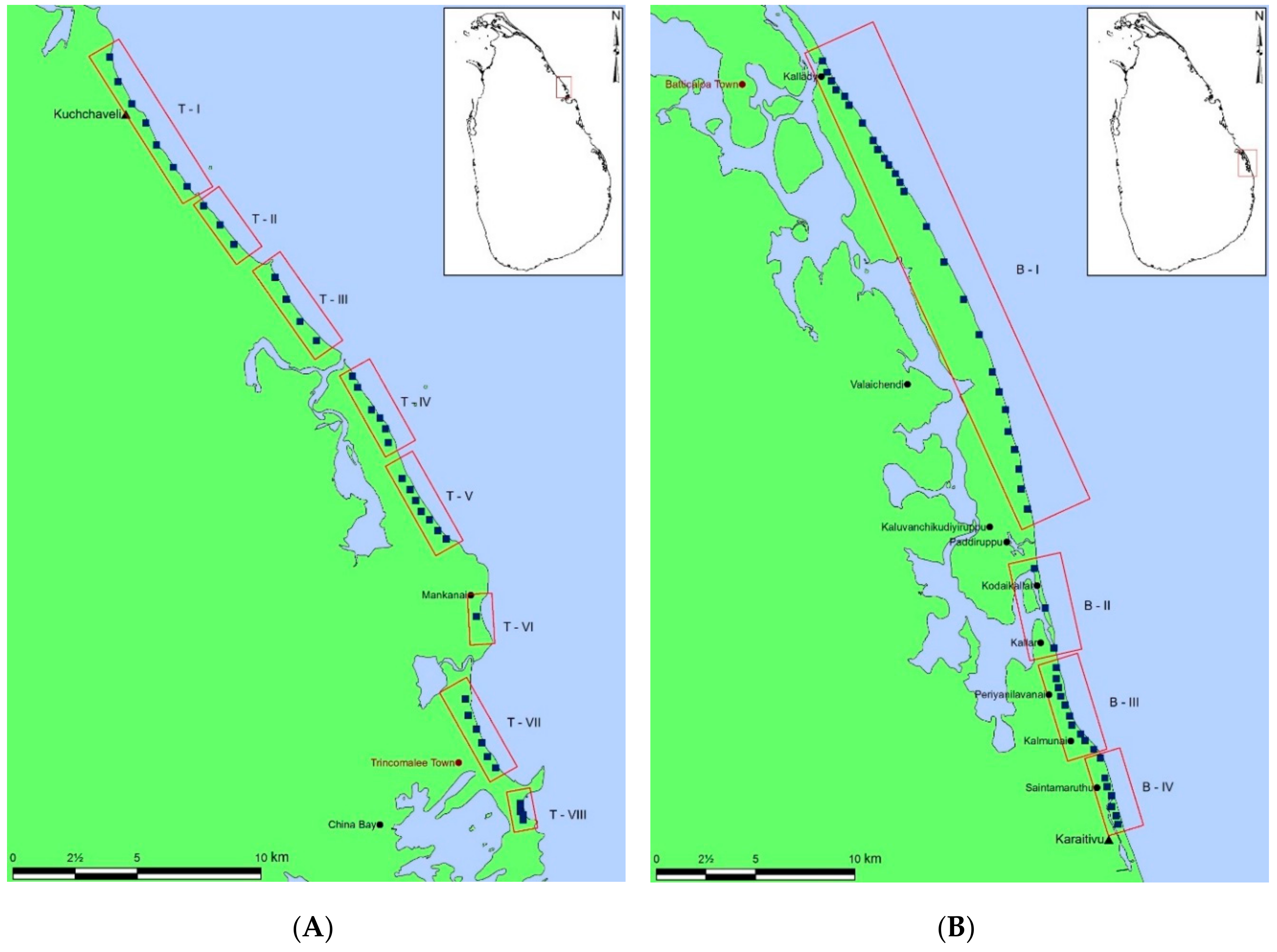
2. Study Site

Sri Lanka’s coastline is 1680 km long, and the country’s geographical location leaves it exposed to storms from several directions that differ in their characteristics according to coastline orientation and season. Furthermore, the coastal zone is extremely low lying (less than 1 m above mean sea level (MSL) up to a distance of 1–2 km inland in most places), leaving it highly exposed to coastal inundation and erosion. At present, large parts of the nation’s coastline suffer from storm erosion regularly, as well as chronic coastline recession [14]. With a projected global sea level rise of up to 1 m above present-day MSL (by 2100) and increased intensity and frequency of storms and storm surges, coastal communities and developments around Sri Lanka will likely be severely threatened by permanent/episodic inundation and/or coastal erosion [15].

The conflict situation that prevailed for more than 30 years in the northern and the eastern districts of Sri Lanka has disrupted proper management of the coastal resources and developments in those regions. Furthermore, the socio-economic status of the coastal communities in the entire country has degraded rapidly due to the conflict situation. However, since the end of the civil conflict in 2009, ample opportunities for economic development, particularly along the coast, have emerged due to the many natural resources of the coastal region. Accordingly, the Government of Sri Lanka (GOSL) has given high priority to developing major economic hubs, maritime facilities, tourism and the energy sector within particularly the severely under-developed and under-utilised northern and eastern coast regions. The rapid development of the tourism industry, especially in the eastern coastal region, is a priority for the GOSL from an economic point of view. However, in order to safeguard the unique environment in the region and environment-related livelihoods of the eastern communities, balancing conservation requirements with development activities is needed. With the marked post-war increase of population in coastal towns and accelerated economic activities in the eastern coastal region, the requirement of an integrated management approach of conserving, developing and sustainable utilization of resources has also been recognised. These plans also include a coastal zone and coastal resource management plan for the country [14].

The eastern part of the country is vulnerable to many natural disasters such as cyclones, storms, chronic coastal recession, and also tsunamis (as evidenced by the December 2004 Tsunami). The majority of the eastern communities and developments are located in Trincomalee, Batticaloa, and Amparai districts, all of which are densely populated, mainly within the coastal belt. The main livelihoods in the communities of these areas are fishery, agriculture or lagoon fishery [16,17].

For this study, two different sites in the east coast of Sri Lanka were selected: Trincomalee and Batticaloa. In this section, these two sites are described. At both sites, a long stretch of sandy coastline is interrupted by headlands, river mouths and (seasonal) tidal inlets.

3. Data Collection and Analyses

This study required several types of data. These data were either measured in the field or sourced from global databases. This section describes the data used and their analysis.

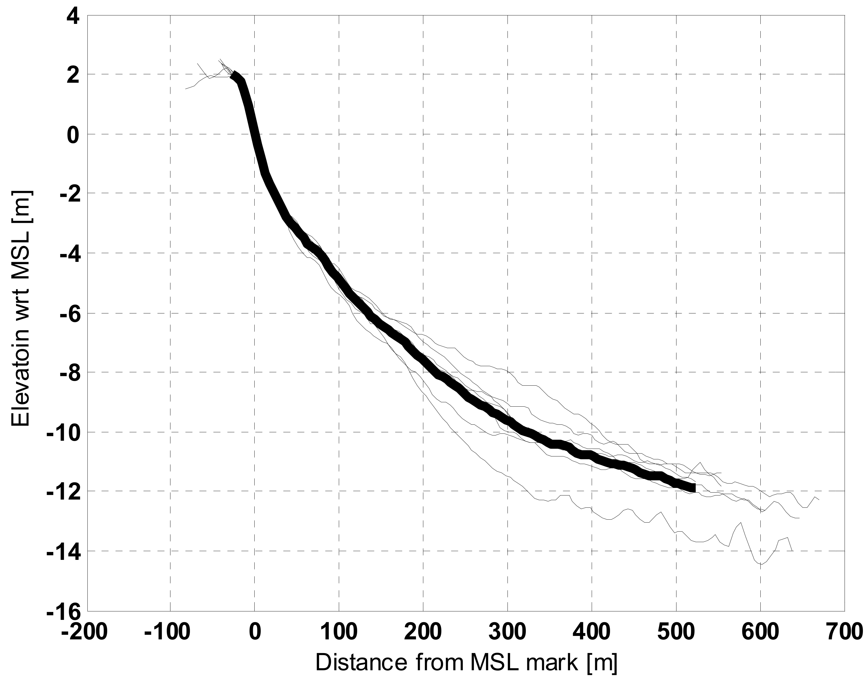
3.1. Beach Profiles and Sediment Size

The most important data that was needed for this study were cross-shore beach profiles along the coastline of the study areas. These data were provided by the Coast Conservation Department (CCD) of Sri Lanka. The beach profiling was done for approximately 100 profiles in Trincomalee and Batticaloa districts. The profiles were measured from the berm or dune at the landward end and continued to a depth of 10–15 m, or an offshore distance or 2.0 km from the beach, with 0.5 to 2.0 km spacing between them. For each profile, the beach/dune height and beach slope was calculated. Figure 2 shows the areas in which the profiles used in this study are located. At each profile location, sand samples were also collected for grain size determination, and sediment grading curves were established for each profile.

Based on the geo-morphological conditions of the coastline along the study areas, we defined 12 coastal cells in total (Figure 2; 8 cells in Trincomalee and 4 cells in Batticaloa). A cell-averaged beach profile was subsequently computed based on the measured beach profiles in each cell. These cell-averaged profiles were then used to calibrate the erosion model. (See Section 4.2). As an example, Figure 3 shows the average beach profile for coastal cell B-IV.

Table 1. Average d50 measured in each coastal cell.

Trincomalee		Batticaloa
Coastal Cell	Ave. d50 (μm)	Coastal Cell	Ave. d50 (μm)
T-I	213	B-I	553
T-II	285	B-II	377
T-III	268	B-V	441
T-IV	323	B-IV	456
T-V	200
T-VI	200
T-VII	240
T-VIII	270

shows the average d50 (intercepts for 50% of the cumulative mass of soil sample) measured in each coastal cell.

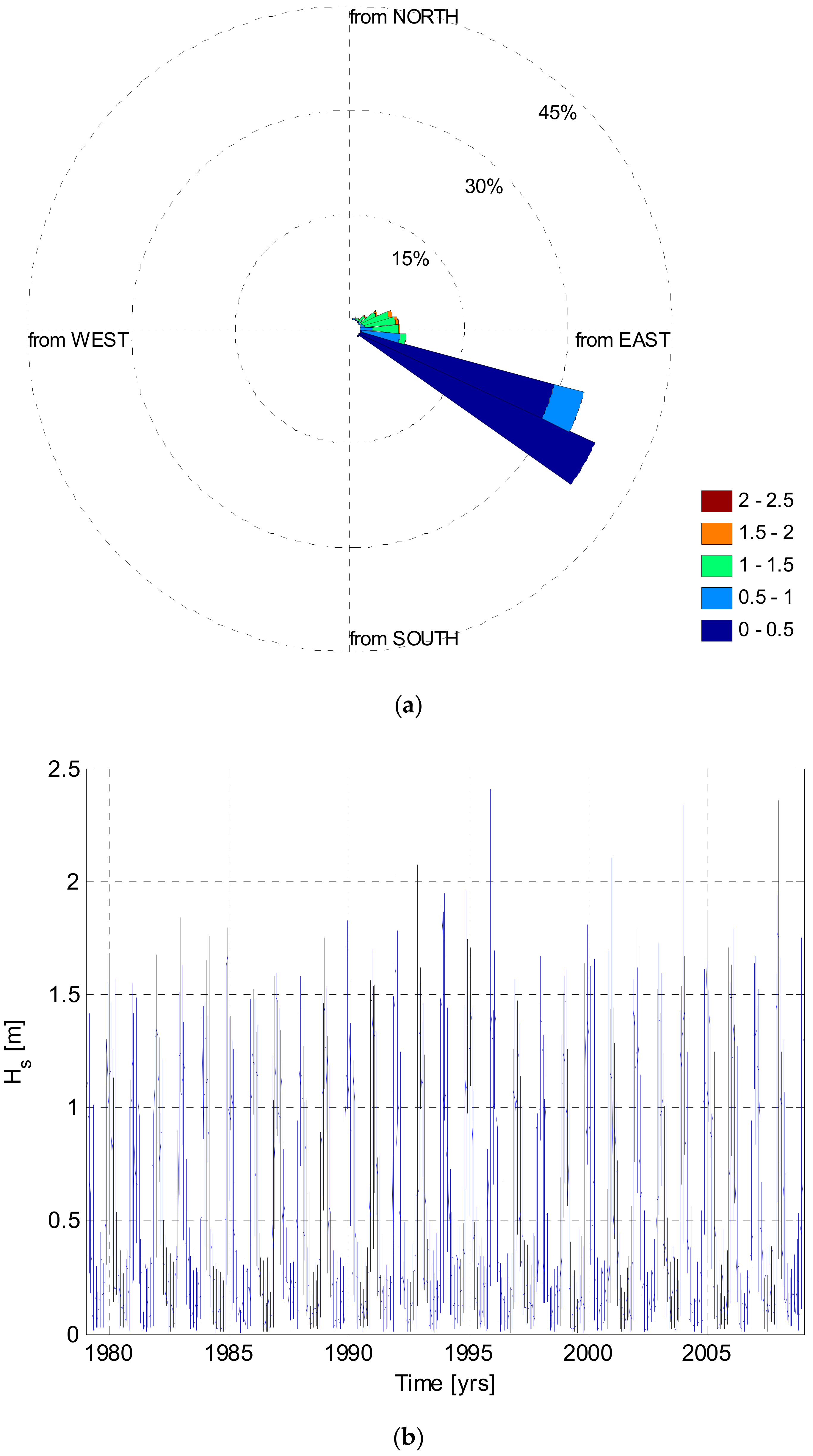
3.2. Wave Data

3.2.1. Off-Shore Wave Data

Since existing local wave data in the study area are of very limited duration, here we used wave data from ERA-Interim (ERAi), which is a global reanalysis providing wave characteristics every 6 h from 1979 till 2016 [18] on a 0.5 × 0.5 degree global grid.

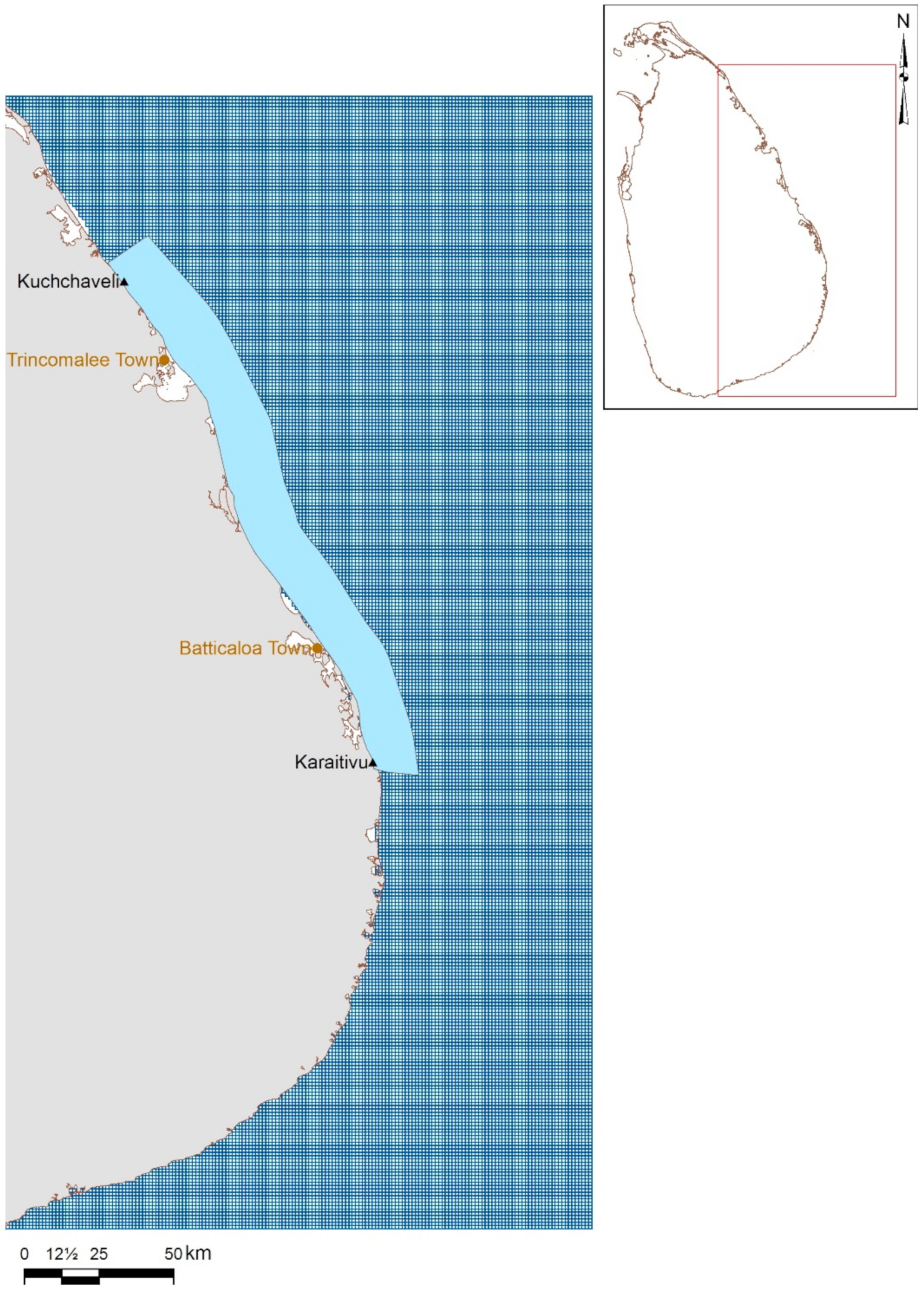
3.2.2. Wave Model

The above-described ERAi wave data is for offshore of the study sites, and thus cannot be directly used in the coastal recession models. Therefore, the deep-water ERAi wave data were first transformed to the nearshore (of the coastal cells defined in Section 3.1) using a 2 dimensional spectral wave model. This section provides a description of the wave model, the model setup adopted for this study, and the results obtained.

The spectral wave model used in this study was SWAN (Simulating WAves Nearshore-model), which is a spectral third-generation wave model (e.g., [19,20]). The SWAN model is based on the discrete spectral action balance equation and is fully spectral (in all directions and frequencies). This implies that short-crested random wave fields propagating simultaneously from widely different directions can be accommodated. SWAN computes the evolution of random, short-crested waves in coastal regions with deep, intermediate and shallow water and ambient currents. The SWAN model accounts for (refractive) propagation and represents the processes of wave generation by wind, dissipation due to white-capping, bottom friction and depth-induced wave breaking and non-linear wave–wave interactions (both quadruplets and triads) explicitly with state-of-the-art formulations. The model has been successfully validated in laboratory and (complex) field cases (e.g., [20,21]). It is noted that the SWAN model does not account for diffraction effects.

In this study, all SWAN simulations were carried out in the stationary mode, with the depth-induced breaking model [22]. To account for bed friction in SWAN, the so called ‘JONSWAP’ model [23] was chosen.

Grid and Bathymetry

To reduce the computational burden and to be able to simulate the phenomena desired in this study, two curvilinear grids were set up: one large-scale regional grid with a resolution of 0.01 degree for the entire east coast of Sri Lanka, and one local grid with minimum resolution of 70 m along the coastline of Trincomalee and Batticaloa. Figure 4 shows the local grid nested within the regional grid. The computational grid in this model covers areas with elevations lower than 2 m above mean sea level.

For the bathymetry of the wave model, data from General Bathymetric Chart of the Oceans [24], which is a publicly available bathymetry of the oceans, were used. GEBCO data (http://www.gebco.net—last visited 30 August 2017) can be projected on grids at different resolution. These data are not very accurate in the nearshore; therefore, GEBCO data were used for the local grid, with the measured profile data (see Section 3.1).

Boundary Conditions and Forcing

Wave forcing was applied at the open boundaries of the model using nearshore transformed ERA-interim wave data, such as significant wave height, peak period and direction, every 6 h. Figure 5 shows the wave-roses of time series of wave conditions applied at the wave model boundary.

Simulation and Results

A full simulation of 30 years (1979–2009) was carried out and 6 h wave conditions in front of each coastal cell were recorded. As an example, Figure 6 shows a time series of wave conditions in front of Dutch Bay, Trincomalee (Cell T-VIII).

As can be seen in Figure 6, the dominant angle of wave incidence is SE, but the height of these waves is very small. These SE waves are the waves generated by the SW monsoon (May–September) and are diffracted and refracted around the island of Sri Lanka. On the other hand, E-NE waves with larger heights and E-NE storms are experienced during the NE monsoon (November–February). In the lower panel of Figure 6 this seasonal signal in the wave height is very pronounced. This trend exists for all the coastal cells in the study area.

Storm Detection

For the purpose of this study, it was necessary to define and detect the storms and their characteristics in the 30 years of simulated wave time series for each coastal cell. To estimate storm conditions the following workflow was applied.

For the time series of wave conditions extracted in front of each coastal cell, the 95th percentile significant wave height value for the period of 1979–2009 was set as the cut-off wave height for a POT (peak over threshold) approach of determining storm events. An event was defined as the interval between an adjacent up-crossing and down-crossing of the threshold wave height. The event characteristics were extracted from the wave time series, being the maximum significant wave height, the average direction, the average period, and duration of the event. The duration was defined as the time difference between moments of up-crossing and down-crossing of the event. If the duration of the event was more than 12 h then the event was flagged as a storm. Figure 6 and Figure 7 show this process for the wave extraction point in front of Dutch Bay (Cell T-VIII). In the case of Dutch Bay, 221 storms were detected in the 30 years of data. The overall number of storms detected over the 30-year analysis period based on this workflow in the different coastal cells is around 225 storms, or an average of around 8 storms per year, and as expected, all occurred during the NE monsoon season.

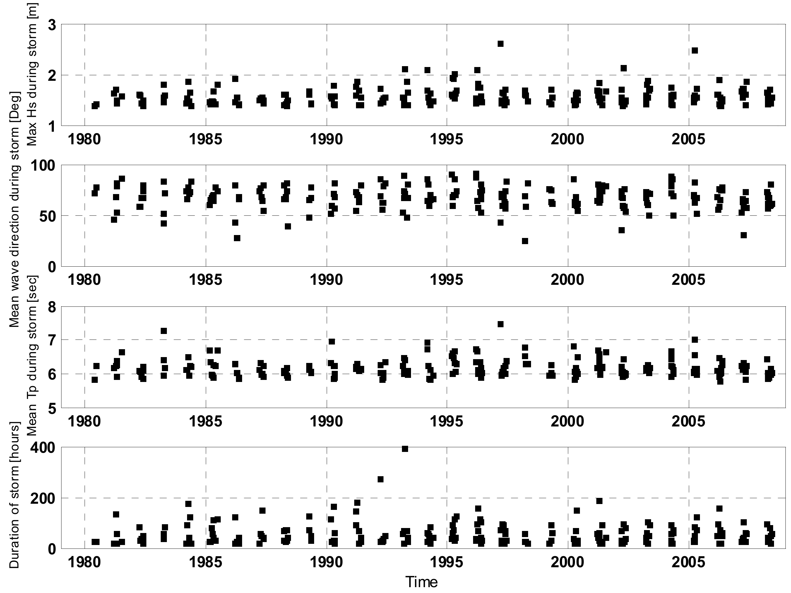
3.2.3. Storm Data Analyses

After detecting storms in all of the coastal cells, statistical analyses needed to be performed on the data. In this section, the methodology which was used for statistical analyses is described using the example of 221 storms detected for Dutch Bay (Cell T-VIII). Figure 8 shows the main storm characteristics for this cell, the maximum significant wave height (Hs) during the storms, and the average peak period of waves (Tp) during the storms, the average wave direction during the storm, and the duration of storms. As shown in Figure 8, storm waves are incident from E-NE (25°–90° Nautical) and occur only during the NE monsoon.

To use these data in coastline recession simulations, a generalised extreme value distribution function (GEV) was fitted to the maximum significant wave height during storms and to the storm durations. Figure 9 shows the cumulative distribution function of GEVs fitted to these variables. Since the wave direction does not have extreme values and for detected storms is limited to a narrow sector, here we used an empirical cumulative distribution function (CDF) for average wave direction during the storms (Figure 9).

To complete the statistical analyses, it is also necessary to check the dependencies between different storm characteristics. Similar to previous studies (e.g., [12]), we chose the maximum significant wave height during the storm as the main parameter and checked its dependencies against the other parameters. Figure 10 shows the dependency between maximum significant wave height during the storm and storm duration and the dependency between maximum significant wave height and average wave direction during the storms. The maximum significant wave height and storm duration are (inter)dependent with higher significant wave heights occurring during the longer storms. On the other hand, the maximum significant wave height and the average wave direction are more or less independent of each other.

To generate a dependency distribution that describes the observed dependency between maximum significant wave height and storm duration, we made use of a copula. A copula is essentially a multivariate probability distribution for which the marginal probability distribution of each variable is uniform; in this study, the ‘Clayton’ copula has been used. Figure 11 shows the joint probability model (JPM) capturing the dependency between maximum significant wave height and storm duration.

For relating the maximum significant wave height and average peak wave period, we used a linear fit of the data, as shown in Figure 12.

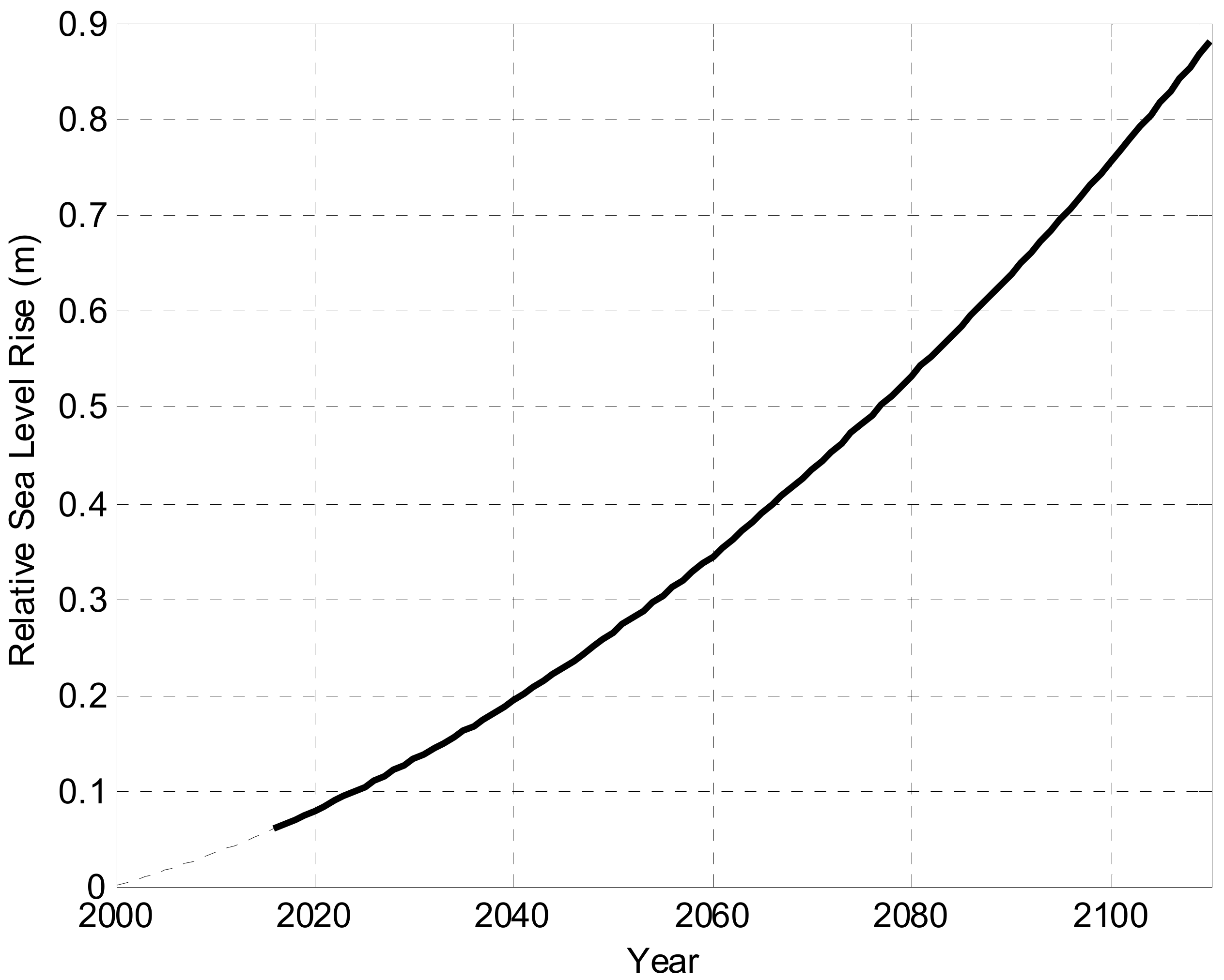
3.3. Relative Sea Level Rise

For the purposes of this study, it was also necessary to estimate the time series of projected sea level rise in the study area. The synthesis report of the IPCC reported that over the period 1901–2010, global mean sea level rose by 0.19 (0.17 to 0.21) m, with an average rate of 1.7 mm/year in the 20th Century [25]. The fifth assessment report of the IPCC [26] indicated a transition in the late 19th century to the early 20th century from relatively low mean rates of rise over the previous two millennia to higher rates of rise (high confidence). From 1961 to 2003, the average rate of SLR was 1.8 ± 0.5 mm/year, while between 1993 and 2010 the rate was very likely higher at 3.2 (2.8 to 3.6) mm/year; similarly, high rates likely occurred between 1920 and 1950. IPCC also reported that ocean thermal expansion and glacier melting have been the dominant contributors to 20th century global mean sea level rise [26]. Relative sea level rise (RSLR) over the next 30–100-year period is the sum of three major components: global-mean sea-level change; regional (local) spatial variations in sea-level change; and vertical land movement (subsidence or uplift). The inclusion of regional components of relative sea-level rise is important when developing scenarios for impact and adaptation assessment as they provide a critical link between global climate change and regional/local coastal management strategies [27,28].

IPCC guidelines to determine local RSLR by 2100 have been prescribed [29], where three different options are given based on data availability. Here, we used the ‘intermediate’ option, together with IPCC AR5 projections of global mean SLR and regional variations in SLR. The suggested ‘intermediate’ assessment methodology [29] was adopted to derive RSLR scenarios linked to the RCP8.5 IPCC scenario by deriving the coefficients the method as follows:

$$SLR= a_{1}t+a_2{t}^2$$

(1)

where:

• SLR is global mean sea level rise (m)
• t is number of years starting from 2000 (year)
• a₁ is rate of sea level rise at year 2000 (m/year) (in this case 0.003)
• a₂ is factor of the change in the rate of sea level rise (m/year²) (in this case 4.5 × 10⁻⁵)

To account for regional (local) spatial variations in sea-level change, the difference between global mean sea level rise and ensemble mean regional relative sea level change between 1986–2005 and 2081–2100 for RCP 8.5 [26], is added linearly to the time-varying SLR estimated using Equation (1). This variation includes effects of atmospheric loading, land ice, glacial isostatic adjustment (GIA) and terrestrial water sources. In these calculations, the land subsidence is ignored due to lack of data.

Figure 13 shows the RSLR values taking into account the global mean SLR and regional variations of SLR for the east coast of Sri Lanka.

4. Application of Probabilistic Coastal Recession (PCR) Simulations

The primary functions of the PCR framework are: randomly generate long (~100 years) time series of storm conditions and the gap between them from pre-determined Joint Probability distributions of storm conditions, calculate erosion during the storm using a profile model, calculate subsequent recovery during the inter-storm periods, and calculate time series of coastline location which is stored as output (Figure 14). This process is repeated ~100,000 times, resulting in the data set necessary for robust statistical analysis [11].

In this study, the (joint) distributions of storm characteristics developed in Section 3 are used to generate the time series of storm conditions and gap between storms (See Section 4.2), and the erosion model of Mendoza and Jimenez [30] (See Section 4.3) is used as the profile model to calculate erosion and coastline retreat.

According to the coast conservation department of Sri Lanka, significant storm surges are very uncommon in the study area. Furthermore, no long-term water level data are available to derive storm surge information in the study area. Recent global storm surge modelling studies [31,32] indicate a 1:100-year return period extreme sea level (combining surge, tide and wave run up) of less than 0.5 m along the east coast of Sri Lanka), and hence storm surges were not considered in this study. Also, since there aren’t any studies that have provided reliable projections of climate change driven variations in extreme waves in the study area, such changes were not considered in the simulations undertaken in this study.

4.1. Event Generation

PCR simulations require a large number of long records of storm conditions and gaps between storms. This means that first, it is necessary to sample single storms, and then construct a time series of storms.

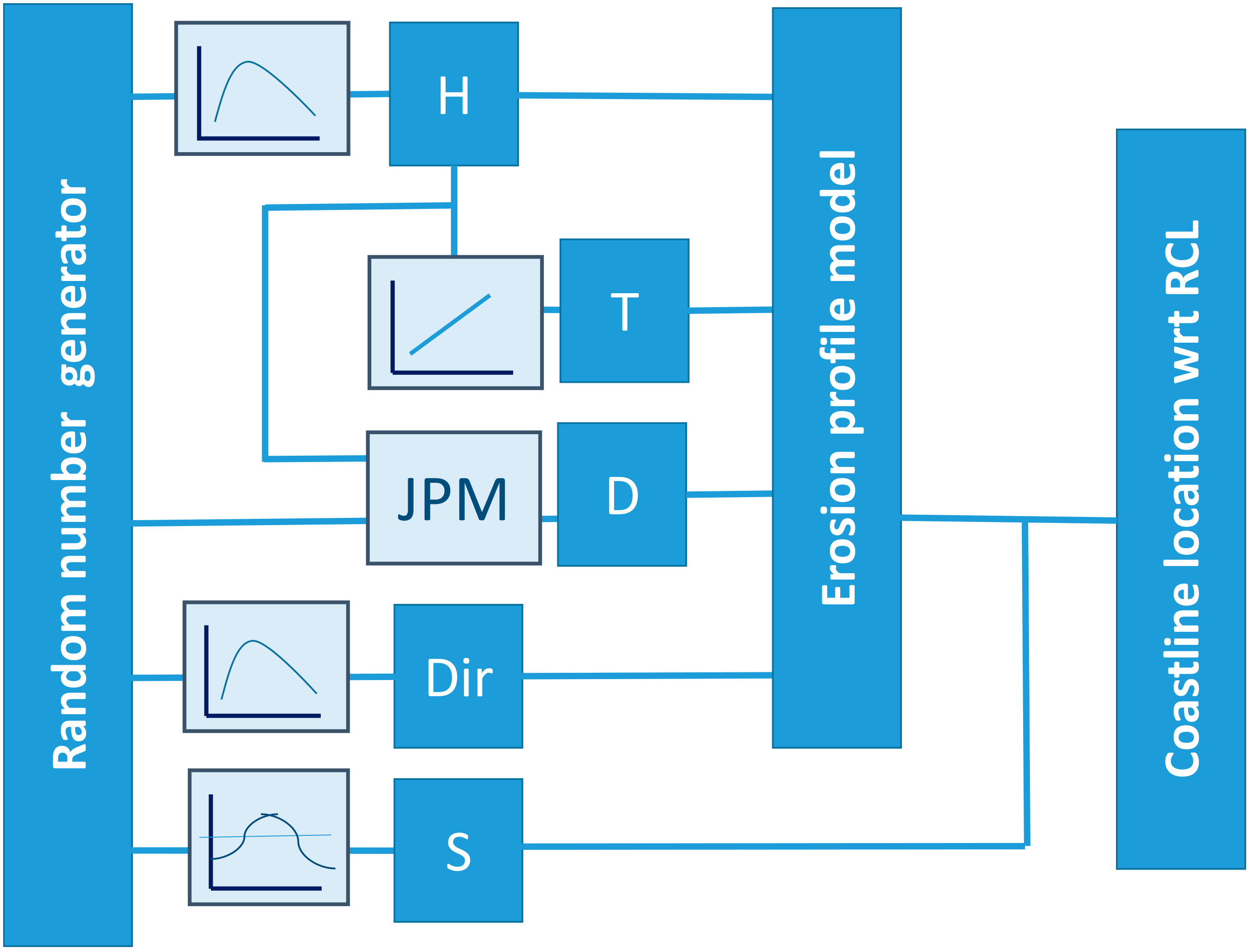
4.1.1. Sampling Single Storm Conditions (H,T,D,Dir)

In summary, to sample a single storm, the following information, which was determined in Section 3.2.2, is required:

• GEV distributions for H_s,max (H) and Storm Duration (D); (e.g., Figure 10)
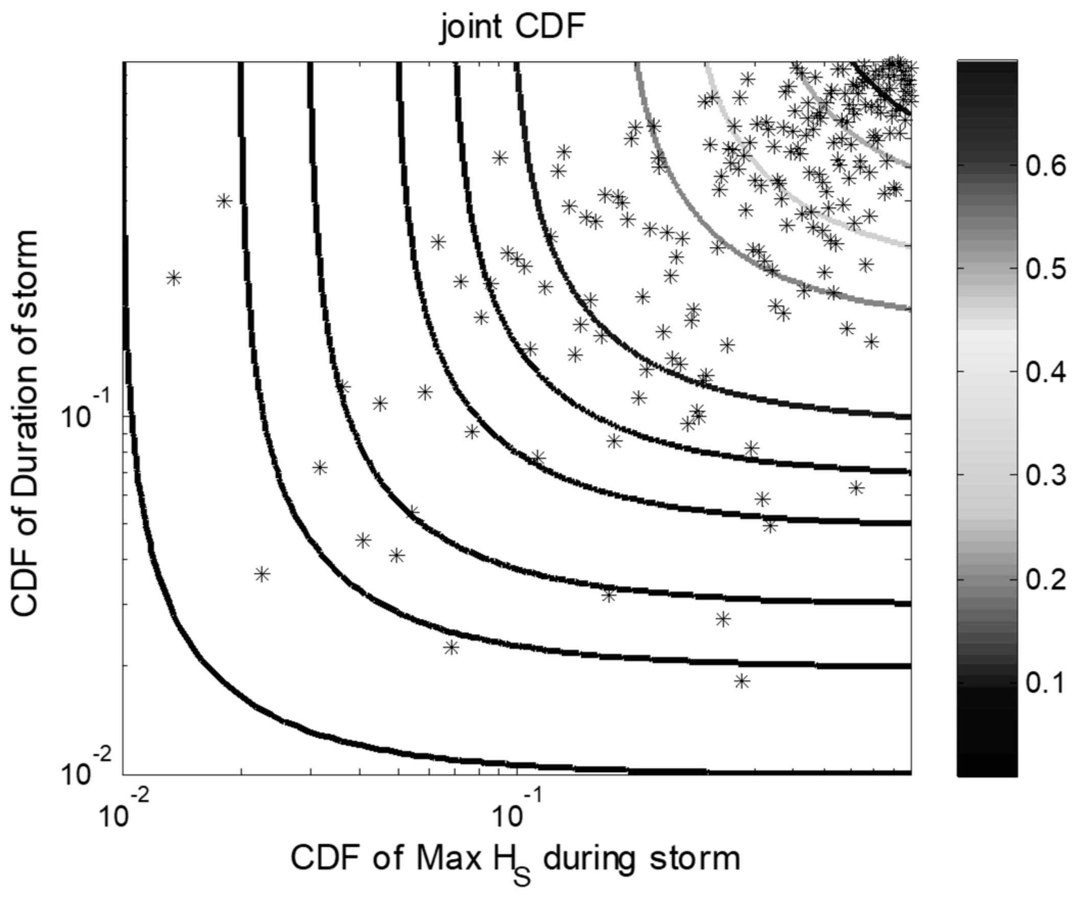
• Joint probability model, characterised by single values of dependency factor between H & D; (e.g., Figure 11)
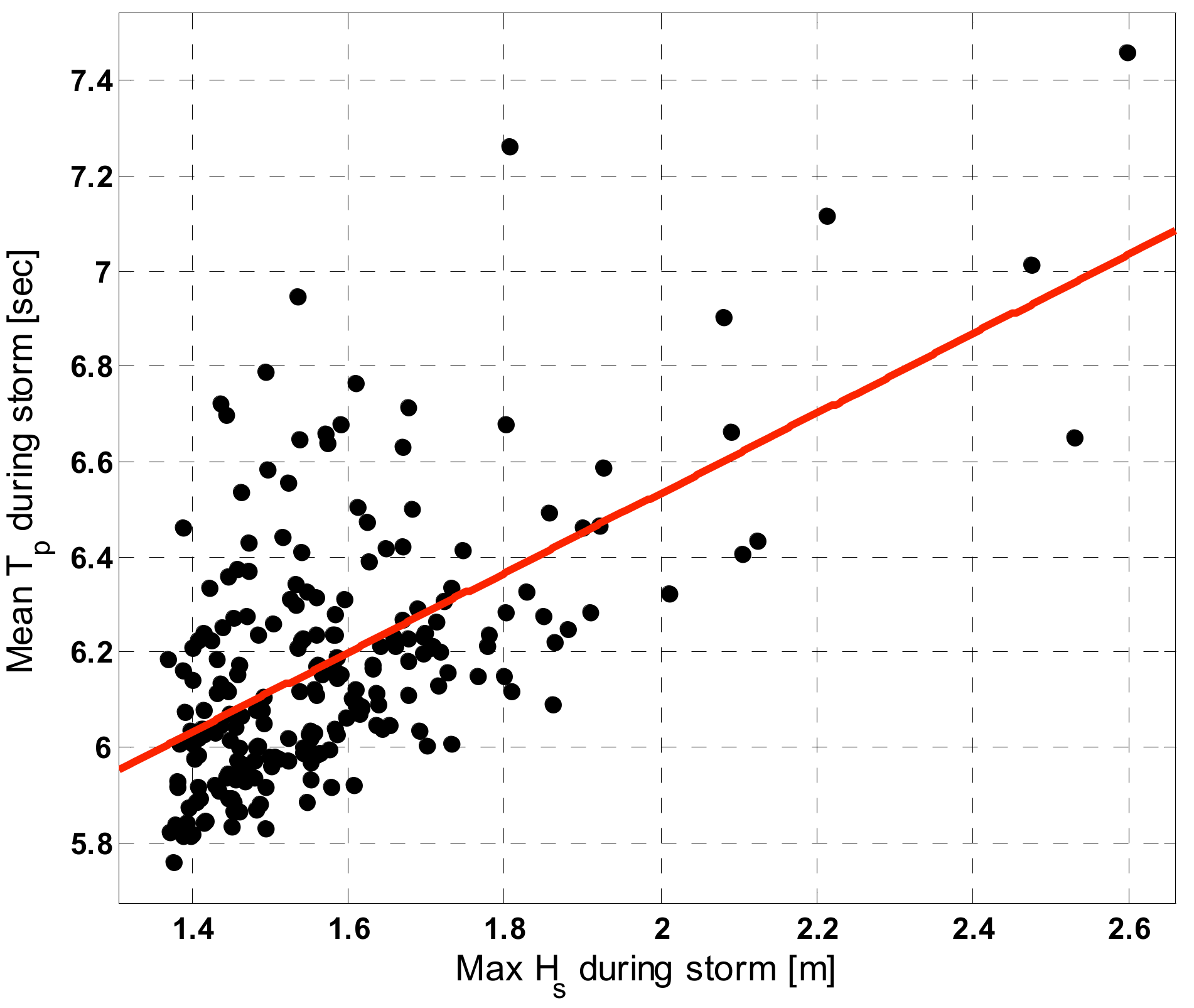
• A linear fit between storm wave peak period (T), which is dependent on H; (e.g., Figure 12)
• An empirical distribution for wave direction (Dir), based on measured data. (e.g., Figure 9)

Using this information, a single storm can be randomly generated as follows:

• Sample a random uniform deviation from [0;1] ‘a’ and use this with the GEV distribution for H to generate a maximum significant for the storm;
• Sample a random uniform deviation from [0;1] ‘b’ as the dependency parameter as dependency value for H and D;
• Use a and b to determine the deviation ‘c’ for storm duration (D) from the joint probability model;
• Use ‘c’ with the GEV distribution for storm duration (D) to generate a storm duration for the storm;
• Use H and the linear fit between H and T to determine storm wave peak period (T);
• Sample a random uniform deviation from [0;1] and use this with the empirical distribution for direction to generate a wave direction for the storm (Dir).

Following this approach, the main storm conditions can be randomly generated from data-fitted distributions.

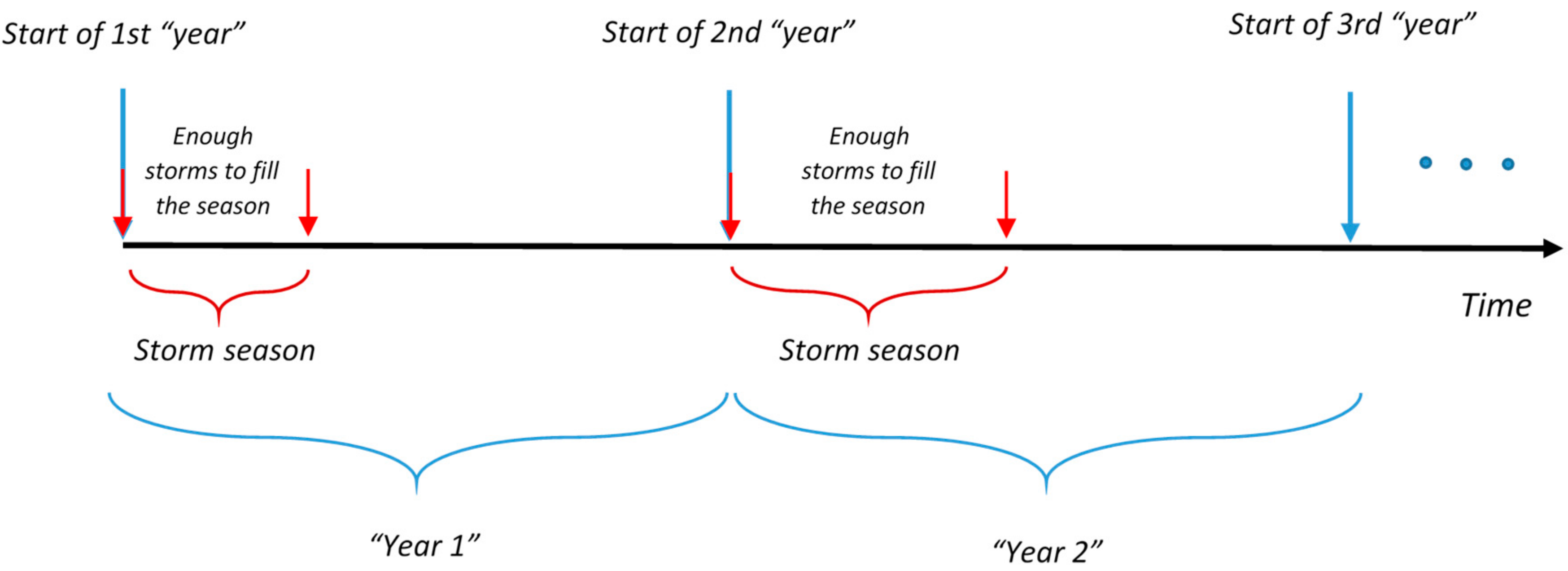
4.1.2. Constructing a Record of Storms Including Seasonality

A typical PCR model simulation requires a simulation length to be selected and a sequence of storms and subsequent gaps during that period to be generated. For example, a typical situation may involve considering the 100-year period (here taken as the period between 2016 and 2116) to assess the impact of climate change over the next 100 years. The series of storms and the gaps between them during this period are then sampled. Storms are sampled using the methods outlined in Section 4.1. The sampling of the gaps between storms is described below.

Due to the strong seasonality of storms in this case, to be able to generate realistic long-term records of storm waves, we considered the following 3 parameters:

• Gap between storms during the storm season;
• Duration of the ‘years’, which is the time from start of the first storm in the storm season until the start of the first storm in the next stormy season;
• Duration of ‘storm season’, which is the time from start of the first storm in the storm season until the end of the last storm in the same storm season;

First, the derived storm time series was analysed to obtain the data set for each of the above-mentioned parameters. Subsequently an empirical distribution function was fitted to the gaps between storms during the storm season and Poisson distribution functions were fitted to the duration of the ‘years’ and duration of ‘storm season’. Then the sequence of storms in a typical simulation length was determined using the following algorithm. Figure 15 shows a schematic of this algorithm.

• Sample a random uniform deviation from [0;1] and use this with the Poisson distribution for Duration of the ‘years’ to generate the duration of one ‘year’;
• Sample a random uniform deviation from [0;1] and use this with the Poisson distribution for Duration of the ‘storm season’ to generate the duration of the ‘stormy season’ in that ‘year’;
• Sample a single storm based on the algorithm described in Section 4.1.1;
• Sample a random uniform deviation from [0;1] and use this with the empirical distribution for gap between storms during the storm season to generate one gap corresponding to the storm generated in pervious step;
• Repeat the previous steps until the duration of the ‘storm season’ is filled with storms;
• Repeat all steps to cover the whole simulation length (e.g., 100 years).

The storm record generated in this way contains the exact time of each storm and, therefore, based on estimated relative sea level rise (Figure 13), it is now possible to determine the MSL at the time of occurrence of each storm.

4.2. Erosion Model

To calculate the coastal erosion and coastline recession in the PCR model, here we used the structural erosion function (model) proposed by Mendoza and Jimenez [30]. This structural erosion function permits the calculation of the magnitude of eroded volume and beach retreat, by means of an aggregated model which depends only on storm properties (Hs, Tp and duration) and beach morphology (sediment grain size and beach slope).

The structural function is derived by relating the storm-induced eroded volumes simulated with the SBEACH model with a coastal morphodynamic parameter. The selected parameter (JA) is a predictor which comprises the Dean parameter and the beach slope [33],

$$J\mathrm{A}={\left|D_{0,e}-D_0\right|}^{0.5}\times m$$

(2)

where D₀ is the Dean parameter (H/T w_s), D_0,e corresponds to its value at equilibrium (2.5 when using deep water waves [34]), w_s is the fall velocity and m is the mean profile slope. This JA parameter was successfully used to predict the magnitude of eroded volumes in beach profile experiments obtained in large wave flumes and, therefore, it is considered a good predictor of storm-induced cross-shore beach profile changes. A linear model is given by Equation (3) [30],

$$\Delta V=C1.JA.dt+C2$$

(3)

This approach can also be used to estimate the shoreline retreat during the storm, by relating the simulated shoreline retreat against corresponding values of the parameter JA.dt. To obtain a representative retreat for the subaerial beach, here we calculate a representative beach retreat ΔX_r as

$$\Delta X_r=\Delta V / \left(B+d^{*}\right)$$

(4)

where B is the berm height and d* is the depth down to which erosion of the inner (landward) part of the beach profile occurs.

One of the main points to be considered when applying this approach is that the erosion structural function needs to be calibrated for the study site to properly fit the coefficients in Equation (3).

Due to the absence of pre- and post-storm erosion data at the study site, here we used the Transact (1D) version of the XBeach model [35,36] to calibrate the structural erosion function of Mendoza and Jimenez [30]. In this study, an XBeach 1D model was used in Surfbeat mode for each coastal cell defined in Section 3.1 and used with the average profile and average D50 of that cell in the model. In XBeach simulations, the Soulsby-Van Rijn sediment transport formulation [37] and avalanching process were used. Following other studies (e.g., [30]), we carried out a range of simulations for different possible predictor (JA.dt) values for each cell. Using a linear fit between resulting ΔV and JAdt, the values for C1 and C2 were determined for each coastal cell. For the profiles in different coastal cells, different calibration factors were applied. Here it was assumed that, between storms, the beach would recover in a such way that, in the absence of climate change, the coastline would remain in place with an exceedance probability of 50%, and after recovery, the profile would reshape to its original shape, and therefore the beach slope (m) and beach height (B) would remain the same. D50 was taken from the available data, and based on XBeach simulations, the d* term was set equal to a water depth of 1 m.

4.3. Definition of Reference Coast Line (RCL)

The value of coastal retreat is only useful in planning if it is benchmarked to a reference coastline. Since the results of PCR modelling are intended for subsequent use in economic risk assessments, all the calculated coastal recession estimates were converted to the distance of the coastline after storm erosion from a reference coastline (RCL). The RCL was defined as the line where the exceedance probability of the run-up, estimated using Stockdon’s runup formulation [38], over the entire 1979–2009 period was 1%. Practically no development is present seaward of this line.

4.4. PCR Simulations

For every coastal cell along the study area, the methodology shown in Figure 2 was implemented to analyse the wave data from the corresponding observation point. PCR simulations were then carried out for every profile in the respective coastal cell (85 profiles in total). The process of constructing a time series of storms and gaps, and then estimating erosion extents from that time series (see Section 4.2 and Section 4.3). The duration of the constructed time series was 96 years (2015–2110) and for each simulation, the most landward location of coastline in each calendar year was recorded.

This enables the construction of an empirical distribution of the maxima of coastline recession for every future year. The simulations needed to be repeated many times before stable results were obtained, especially at lower exceedance probabilities. In practice, for each profile, 100,000 simulations of 96 years were undertaken.

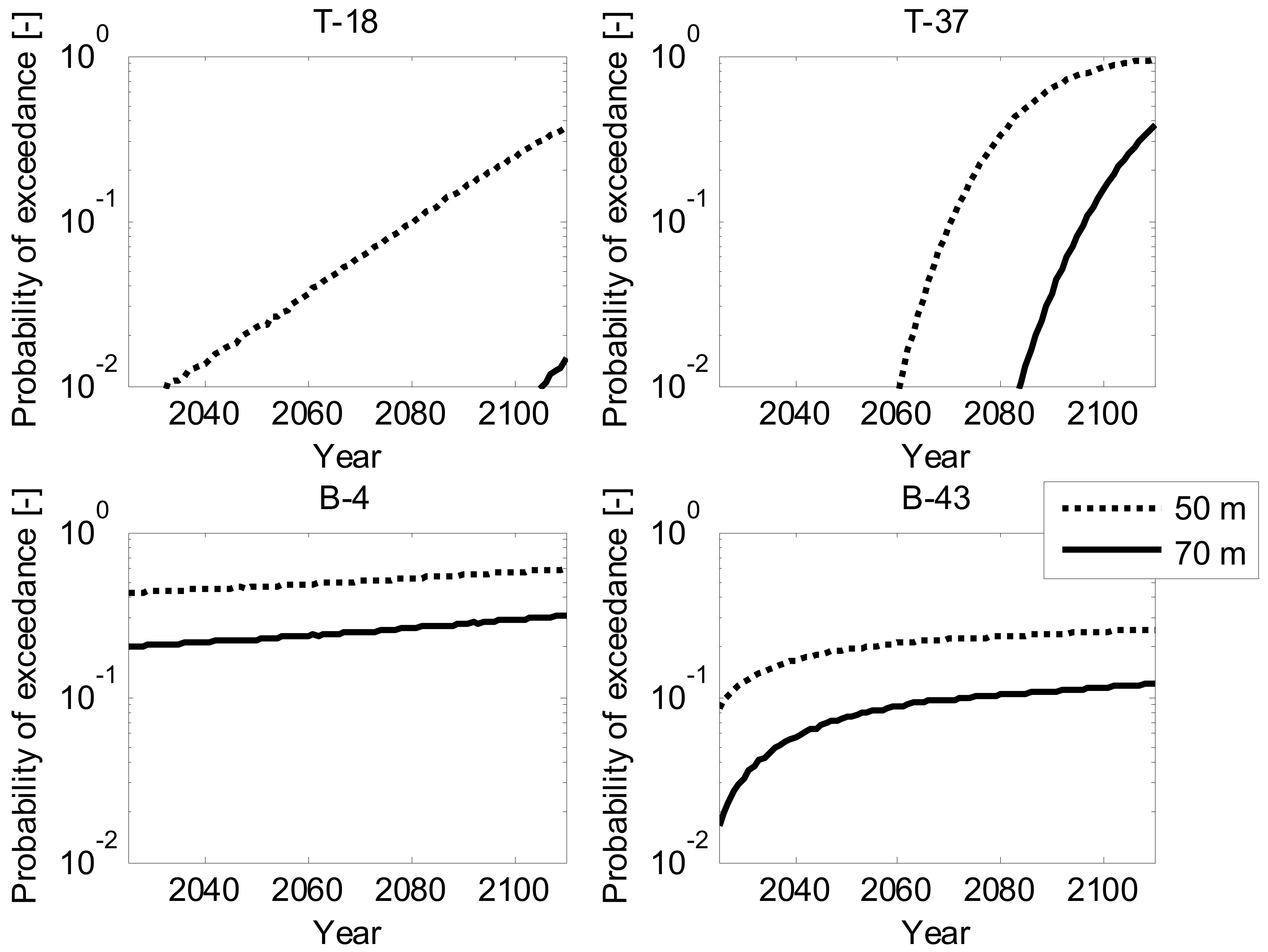
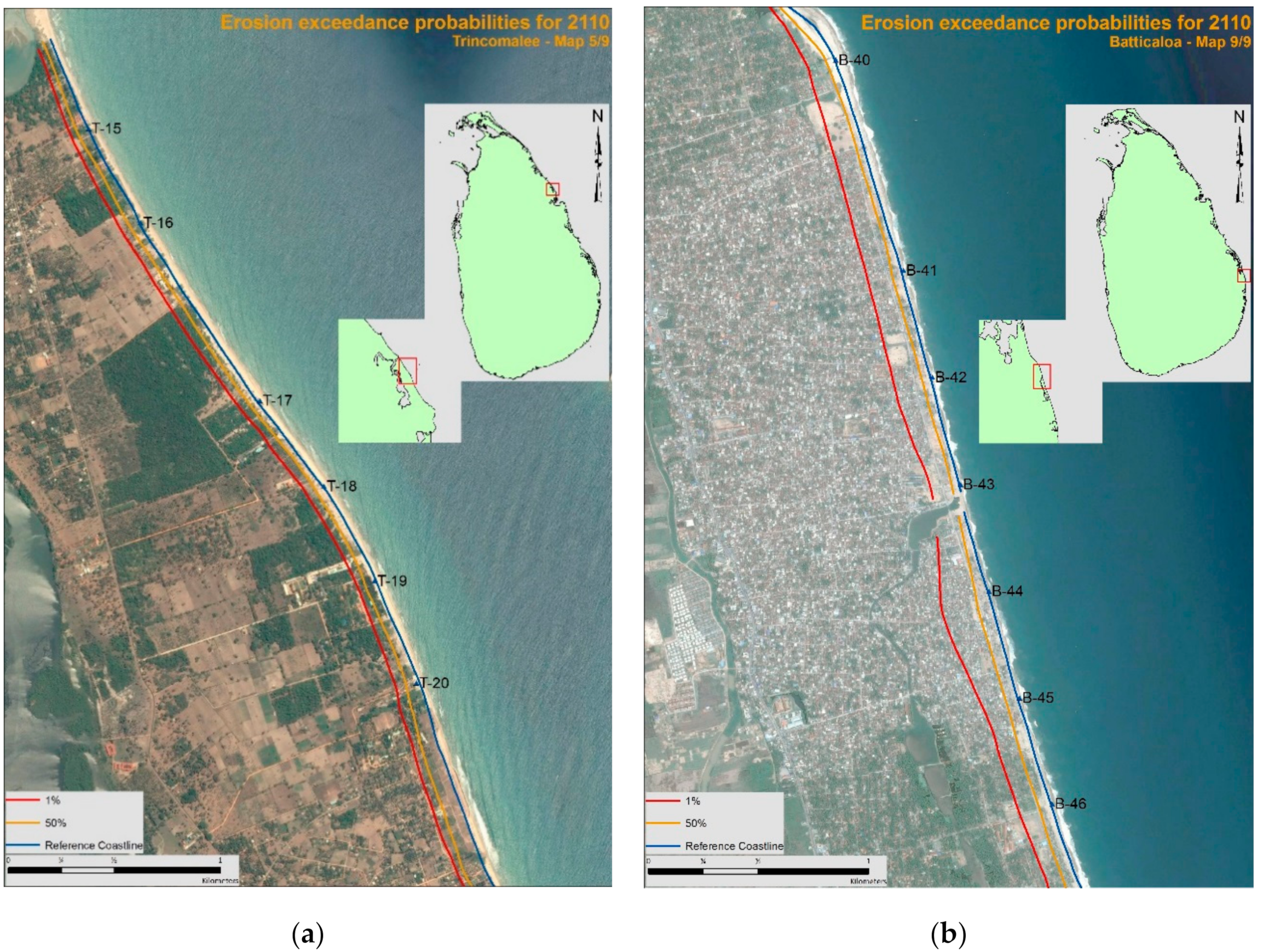
4.5. Results and Discussion

For illustration purposes, here the results of 4 different profiles (T18, T37, B4 and B43) are discussed in detail. Figure 16 shows the exceedance probability curves of coastal recession for these profiles in different years—2025, 2050, 2080 and 2110—and

Table 2. Coastal recession magnitudes (m) associated with different exceedance probabilities in 2050 and 2110 for selected profiles.

Profile	2050			2110
	Probability of Exceedance			Probability of Exceedance
	1%	10%	50%	1%	10%	50%
B-4	142	89	48	149	98	56
B-43	109	64	28	132	75	32
T-18	54	42	29	72	60	47
T-37	41	34	26	91	80	67

gives the values of coastal recession for different exceedance probabilities in 2050 and 2110. For example, Table 2 shows that the probability that coastal recession exceeds 48 m in year 2050 in profile B-4 is 50%. Figure 17 presents the same results, but in a format that is more useful for the public and decision-makers; this shows the increase in the annual probability of coastal recession reaching a fixed location with defined distance from RCL (50 m and 70 m). These types of results for every profile along the study sites, for every meter from the RCL, are used as the input for the economical optimization model. Examples of maps showing the 1% and 50% exceedance probability coastal recession contours are shown in Figure 18.

Based on the similar results obtained for all of the 85 modelled profiles, maps of 1% and 50% exceedance probability coastline recession contours were computed for the Trincomalee and Batticaloa study areas. For Trincomalee, the 1% exceedance probability coastline recession in 2110 varies between 37 and 192 m, and for Batticaloa, between 69 and 262 m.

In this study, we used a JPM function between the wave height at the peak of the storm and the storm duration. There are other more complicated methods for the random generation of storms that link more parameters of the storm, e.g., wave height, peak period, total storm energy and wave direction, using multidimensional copulas and mixture Von Mises Fisher distributions. This leads to the generation of wave storm components with a common dependence structure (e.g., [39]). These methods can indeed be applied in the random storm generation of a PCR framework. Also, the choice of erosion model may have an effect on the results. However, in the absence of any storm erosion data, quantifying such effects is not feasible.

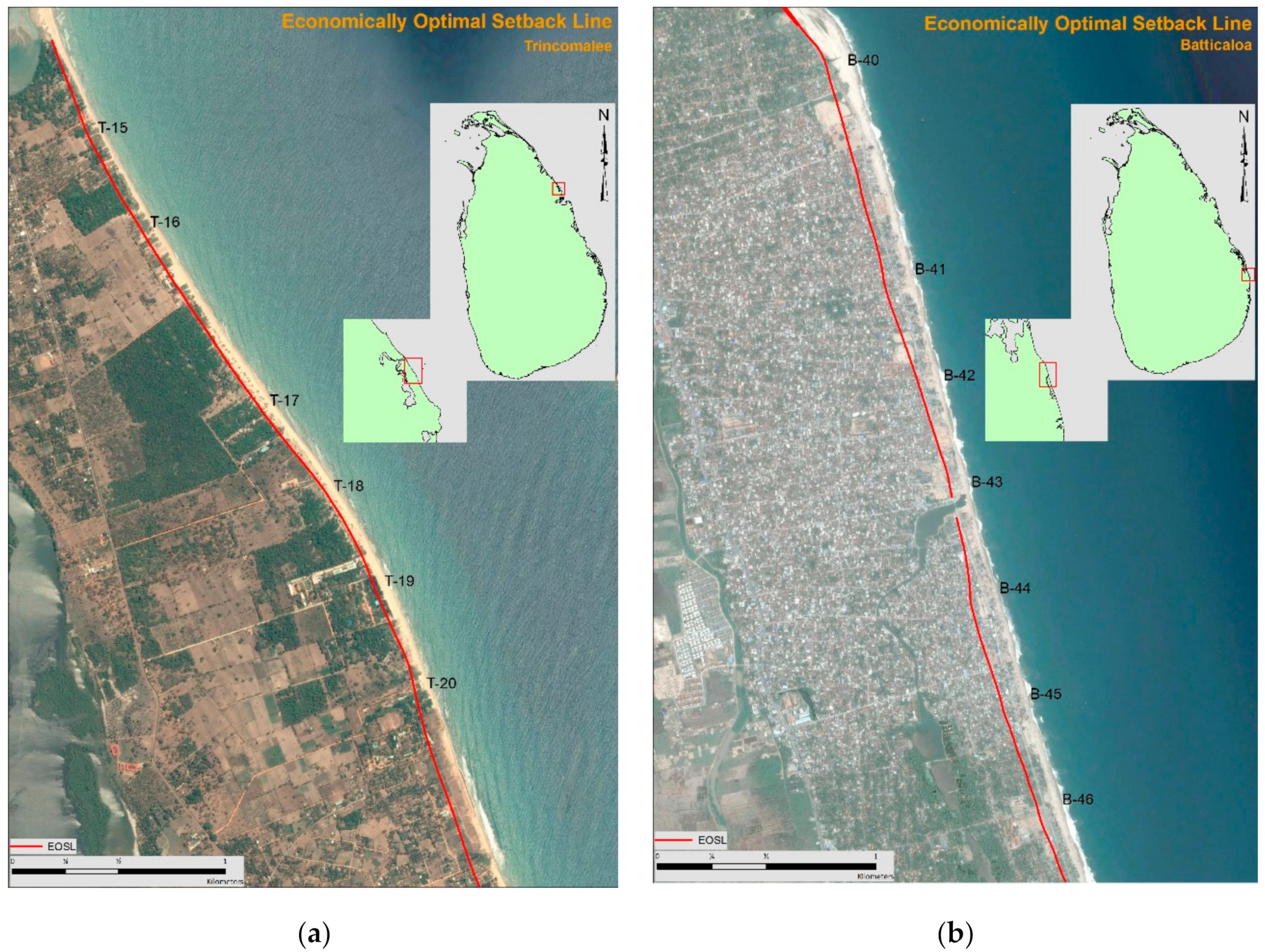
5. Economically Optimal Setback Lines

5.1. Economic Model

The risk of coastline erosion is mostly an economic issue. Forgoing land-use opportunities in the coastal zone is costly, but so is damage caused by erosion. This makes the establishment of setback lines a balancing act. Positioning a setback line farther inland reduces the economic risk, but increases the associated opportunity cost.

In a world without market imperfections, no individual would invest in a place where the risk of coastline recession would be too high from an economic perspective. In such a world, there would be little reason for governments to intervene and implement setback lines. In practice, however, incorrect risk perceptions [40], irrational behaviour [41], and/or explicit or implicit government guarantees [42,43] may lead to excessive risk-taking, i.e., over-investment in the coastal zone. Governments could stem such over-investment through financial incentives, such as the introduction of a compulsory insurance scheme. The cost of risk bearing would then be factored into the investment decisions of individuals and firms. Alternatively, or additionally, governments could establish setback lines as a means to avoid development close to the coastline. This is, indeed, what is widely done to prevent excessive risk-taking in coastal zones.

An estimate of the optimal position of a setback line (or, the economically optimal balance between risk and reward) can be obtained from the would-be behaviour of rational, well-informed, profit-seeking individuals in a world without market imperfections. Such an economically optimal setback line (EOSL) can serve as a reference for coastal zone managers/planners, who have to make on-the-ground decisions on implementing appropriate setback lines.

Hereafter, we assume the following:

• Property owners value the risk of coastline recession at expected loss or a multiple thereof. In the presence of efficient insurance markets, the insurance premium would be equal to expected loss, i.e., the product of the probability of damage and potential loss. In that case, every risk-averse individual would purchase insurance. CCD has indicated that the Sri Lankan government is under no circumstances liable for damage caused by coastal erosion. Still, according to the CCD, insurance penetration is low. While this could be due to people’s risk preferences, it could also be due to the unavailability of efficiently priced insurance coverage, mistrust or incorrect risk perceptions. Since people are typically risk-averse, here we value the economic risk as a multiple of expected loss.
• The impact of coastline recession on a property is assumed to be proportional to the footprint of the property being impacted by coastline recession.
• Each property that is impacted by coastline recession is damaged completely.
• Damages are restored to their initial condition following a recession impact. This implies that insurance pay-outs cannot be put to alternative use.
• Restoration takes place in the year in which damage occurs, in the period following the storm season.

The importance of the abovementioned assumptions can easily be investigated via sensitivity analysis, e.g., by increasing or reducing the cost of risk bearing or by varying the discount rate. The optimization procedure itself could also be elaborated to accommodate site-specific conditions and a wider range of decision alternatives, such as protecting sites or nourishing beaches, rather than establishing buffer zones/limiting development. The fact that alternative risk reduction measures (other than set back lines) have been ignored is conservative in the present context, since it implies that future risks may have been overestimated (in the event that protection works were to be implemented).

Under the assumptions above, the net present value NPV(x) of investing at a distance x from today’s coastline equals the sum of the investment cost, the present value of the returns on investment and the present value of the cost of risk bearing:

$$NPV\left(x\right)=-c(x)+{\displaystyle \sum _{i=1}^n\frac{c(x)\times r(x)}{{\left(1+\gamma \right)}^i}}-{\displaystyle \sum _{i=1}^n\frac{a\times c(x)\times p_i(x)}{{\left(1+\gamma \right)}^i}}$$

(5)

where,

• NPV(x)—The net present value of an investment at a distance x from today’s coastline.
• γ—Discount rate.
• p_i(x)—The probability of damage at distance x in year i. This is the probability in year i that the coastline recedes up to a point that is at least a distance x from the reference coastline.
• c(x)—The investment that is made at a distance x from the initial coastline.
• a—The ratio of the certainty equivalent to expected loss. The certainty equivalent is the certain loss that is valued the same as the probability of suffering a loss. For a risk-neutral agent, the certainty equivalent is equal to the expected loss. The factor a could thus be perceived as a risk aversion coefficient.
• r(x)—Rate of return on the initial investment without accounting for coastline recession risk. The product r(x)·c(x) equals an annual return on investment measured in money (e.g., dollar) terms.
• n—The time horizon being considered in years. The value of n equals the number of years in which the return on investment exceeds the certainty equivalent of the risk of coastline recession. This is consistent with the assumption that investors do not willingly incur avoidable losses, but walk away when risks become too high. For practical reasons, we have ignored all cash flows beyond the year 2110, which is the last year for which recession estimates are here computed from the probabilistic coastline recession model.

When the rate of return on investment does not decrease towards the coastline, the economically optimal exceedance probability of today’s economically optimal setback line, i.e., p₁(x), can be found at a position x, where the net present value NPV(x), as defined by Equation (5), drops below zero. This exceedance probability follows from:

$$-c(x)+{\displaystyle \sum _{i=1}^n\frac{c(x)\times r(x)}{{\left(1+\gamma \right)}^i}}-{\displaystyle \sum _{i=1}^n\frac{a\times c(x)\times p_i(x)}{{\left(1+\gamma \right)}^i}}=0$$

(6)

or (after dividing by c(x)):

$$-1+{\displaystyle \sum _{i=1}^n\frac{r(x)}{{\left(1+\gamma \right)}^i}}-{\displaystyle \sum _{i=1}^n\frac{a\times p_i(x)}{{\left(1+\gamma \right)}^i}}=0$$

(7)

When the rate of return and the probability of damage are both the same from year to year, n→∞ and Equation (7) reduces to (note that $\underset{n\to \infty }{\lim }{\displaystyle \sum _{i=1}^n\frac{1}{{\left(1+\gamma \right)}^i}}=\frac{1}{\gamma }$):

$$p_i(x)=\frac{r(x)-\gamma }{a}$$

(8)

Equation (8) follows the intuitive logic that investors would not willingly expose themselves to the risk of coastline recession when the cost of risk bearing is greater than the reward. For example, if risk were valued at expected loss (a = 1) and an investment in a coastal zone were to yield a 0.05 annual rate of return compared to 0.03 for an identical investment at an inland location, the efficient setback line would have an exceedance probability of 0.05 − 0.03 = 0.02 per year. The probability of damage thus essentially acts as a hurdle rate.

The above is illustrated in real-life by fishermen that live as far from the coast as they can without losing sight of their boats. When closeness to the sea offers few benefits and mostly poses risks, it is rational to stay as far away as possible. The same logic explains why luxury hotels can be found along the seafront: closeness to the sea attracts tourists (beach amenity); for luxury hotels, closeness to the sea brings rewards that outweigh a relatively high risk of coastline recession.

When the risk of coastline recession is likely to increase over time due to, e.g., climate change, it becomes economically optimal to introduce a safety margin by lowering the exceedance probability of the setback line that is used for guiding today’s land-use planning decisions.

The position of the economically optimal setback line for future investment decisions differs from the position of the EOSL for today’s investment decisions. This is because of sea level rise and other trends. This implies that the position of the EOSL should be re-evaluated periodically. Here, we consider the position of the EOSL for the year 2025, taking into account the PCR-output for the period 2025–2110. The EOSL for the year 2025 is the optimal setback line for investments made in the year 2025. While this setback line is somewhat conservative for planning decisions prior to 2025, it provides a stable basis for land-use planning decisions over the next decade or so. The EOSLs thus determined range between 12 m and 175 m from the coastline. It is stressed here, however, that the EOSL position should be re-evaluated periodically (e.g., every 10–20 years).

5.2. Economic Constants

Future rates of return on investment, discount rates and risk preferences are uncertain, especially over periods of 50 years or more. These variables could be treated as stochastic, characterised by probability distributions. Since such a fully probabilistic treatment may trigger discussions about the probabilities assigned to alternative future economic developments, we established base case parameter values and investigated the sensitivity of the EOSL changes in these values. The base case parameter values are the values that were used for determining the EOSL for the different sites. Each site was classified as a high-value zone (e.g., urban area) or a lower-value zone (e.g., rural area). The base case parameters yield somewhat conservative results if all combinations of parameter values are considered equally likely, as discussed in Section 5.4. The parameter values that have been considered are shown in

Table 3. The inputs of the sensitivity analyses related to the economic constants.

Variable	Trincomalee		Batticaloa
	High-Value Zone	Lower-Value Zone	High-Value Zone	Lower-Value Zone
Rate of return on investment relative to the discount rate (Δr) (per year)	0.09 0.12 (base case) 0.15	0.05 0.07 (base case) 0.09	0.03 0.05 (base case) 0.07	0.01 0.02 (base case) 0.03
Discount rate (γ) (per year)	0.02 0.03 (base case) 0.04 0.05
Ratio of the certainty equivalent to expected loss (a) (-)	1.0 (risk-neutral) 1.5 (moderate degree of risk-aversion) 2.0 (base case)

.

The parameter values shown in Table 3 are based on information provided by the CCD, historical records of the Sri Lanka core inflation rate and the prime lending rate reported by the Central Bank of Sri Lanka, and anticipated future economic developments. To avoid rates of return on investment that are smaller than the discount rate, the rate of return was defined as r = Δr + γ, with Δr > 0.

5.3. Results: The Position of the EOSL and Optimal Damage Probabilities

The calculated position of the 2025-EOSL relative to the reference coastline is shown Table 3 for the profiles in Trincomalee and Batticaloa, assuming base case parameter values. The reference coastline (RCL) is the coastline at the start of our simulations in the year 2016. The position of the EOSL varies considerably from profile to profile.

The development of the probability of damage over time at the EOSL is shown in Figure 18 (Trincomalee) and Figure 19 (Batticaloa) for different profiles by continuous lines. For all profiles, the probability of damage at the EOSL increases over time because of, among other things, the effect of sea level rise.

The increasing annual probabilities of damage limit the economic lifetime of a development in the coastal zone. After several years, retreat becomes optimal (note that we conservatively ignore protection as an alternative risk management strategy). This happens when the cost of risk bearing starts to exceed the return on investment, i.e., when a·p(x)·c(x) ≥ r·c(x) or p(x) ≥ r/a, see also Equation (5). For instance, at high-value locations in Batticaloa, the cost of risk bearing starts to exceed the return on investment when the probability of damage becomes greater than 0.08/2 = 0.04 per year. At moderate/lower-value locations in Batticaloa, retreat becomes optimal when the probability of damage becomes greater than 0.05/2 = 0.025 per year. In Trincomalee, these limiting probabilities are 0.15/2 = 0.075 per year and 0.1/2 = 0.05 per year, respectively. These optimal values have been indicated by dashed lines in Figure 18 and Figure 19. Retreat becomes optimal when the probability of damage at the EOSL starts to exceed the probability of damage at which retreat becomes optimal, i.e., when the continuous and dashed lines cross.

As indicated by Figure 19, the optimal investment horizon for a development at or close to the EOSL is on the order of 20 years (starting from 2025) in Trincomalee. In Batticaloa, it is on the order of 50–80 years, see Figure 20. This difference arises from the relatively rapid changes in the probability distributions of coastline recession in Trincomalee, in combination with relatively high rates of return on investment. High rates of return of investment make short-term investments profitable. Maps of EOSLs were thus determined for Trincomalee and Batticaloa study areas. Examples of these maps are displayed in Figure 21.

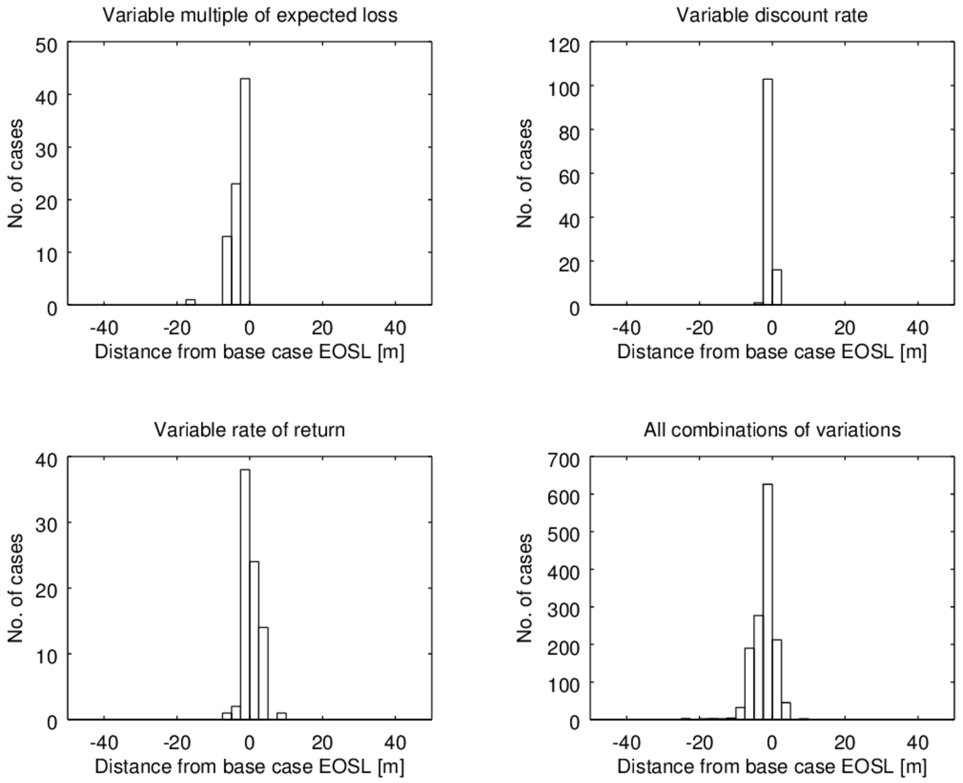
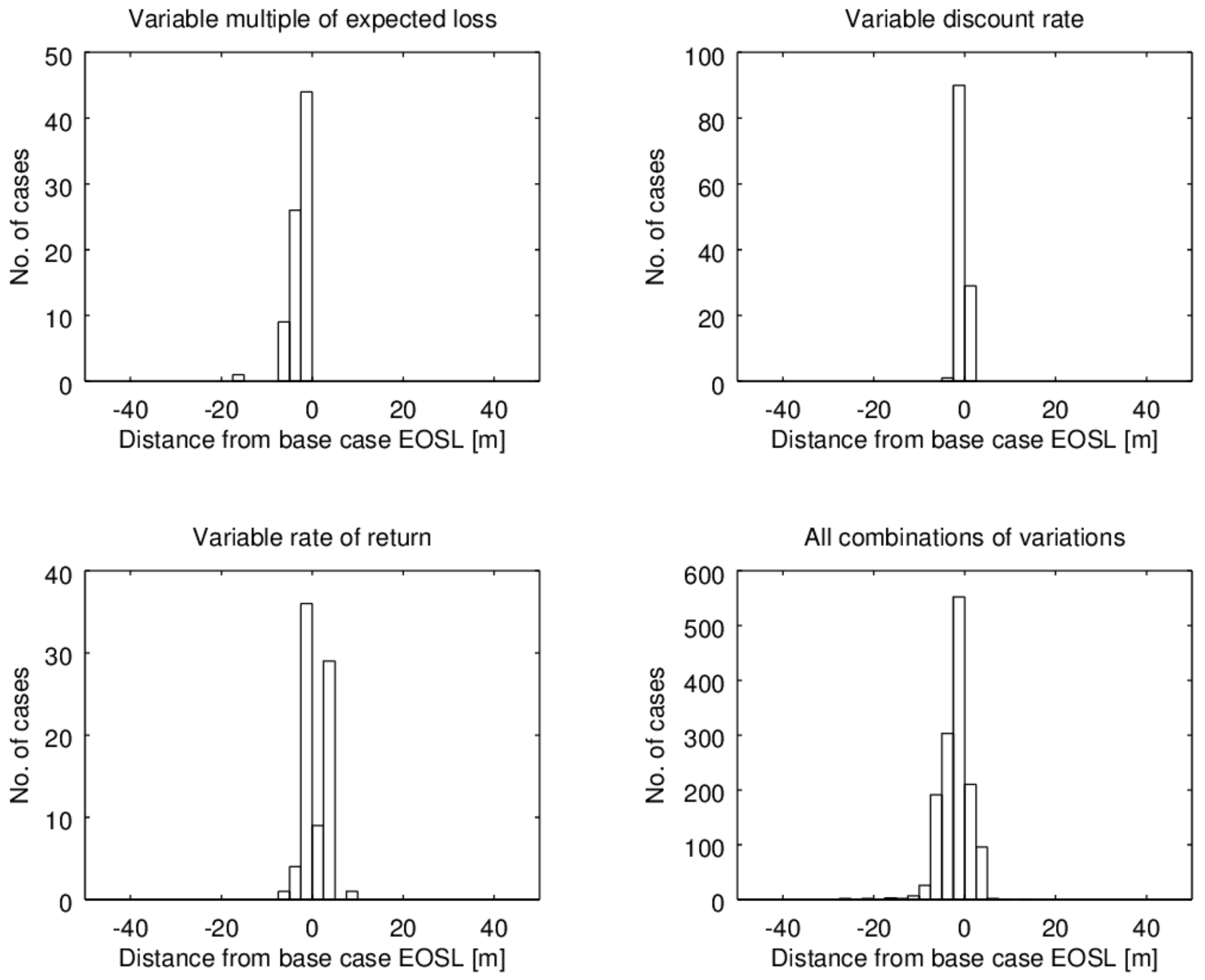
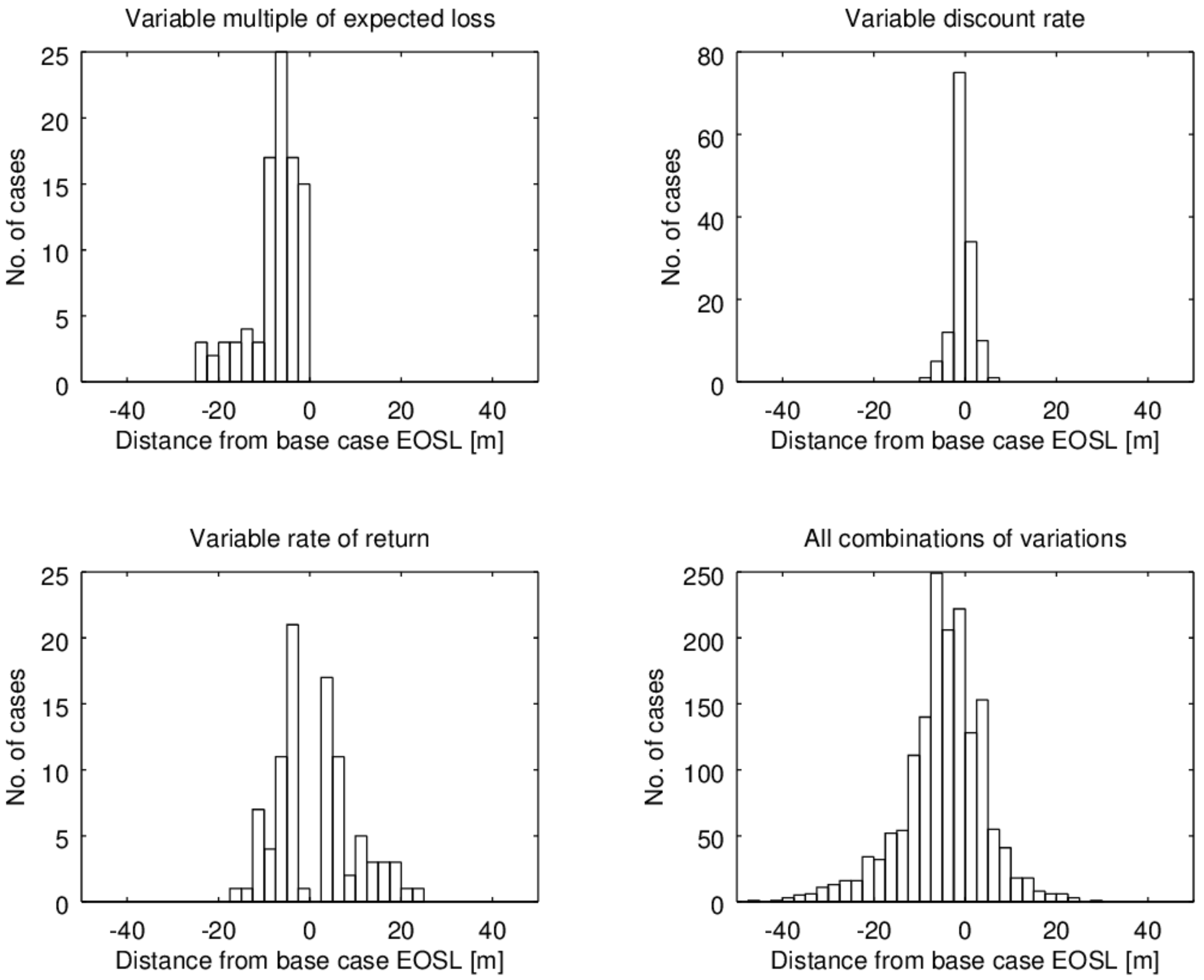
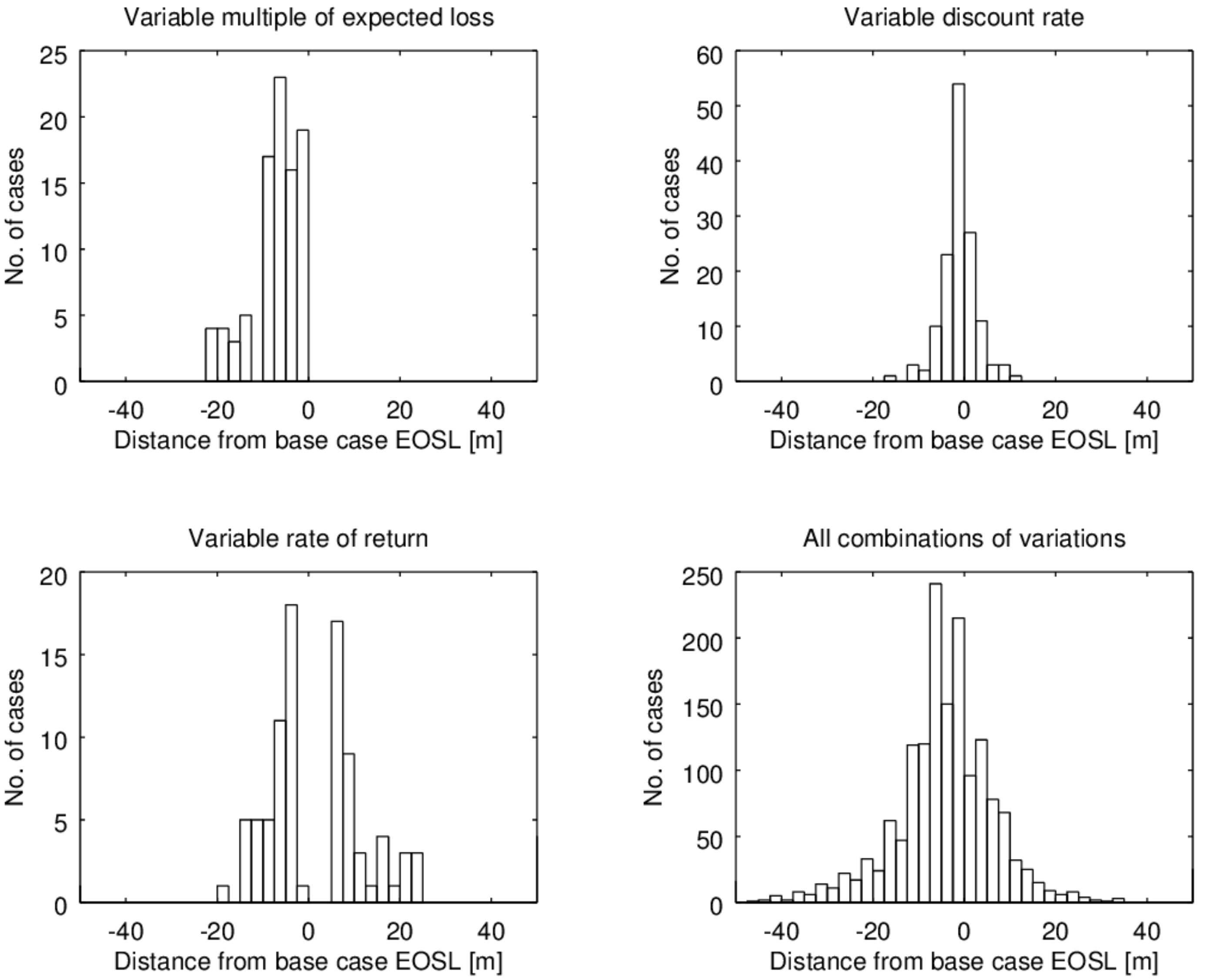
5.4. Sensitivity to Variations in Economic Constants

The results of the sensitivity analyses are shown in Figure 22 and Figure 23 for Trincomalee and in Figure 24 and Figure 25 for Batticaloa. In each figure, the first three panels show the effect of varying a single parameter on the position of the EOSL. The last panel of each figure shows the combined effect of varying the economic constants simultaneously. These figures illustrate the following:

• Decreasing the ratio of the certainty equivalent to expected loss (a) gives the risk of coastline recession less weight and shifts the EOSL seaward. In the sensitivity analyses, we only considered values of a that were smaller than the base case value. This is why the plots only show differences of less than zero. A negative value on the horizontal axis implies the EOSL of the sensitivity analysis lies seaward of the EOSL based on the base case parameter values.
• Increasing the rate of return on investment relative to the discount rate (Δr) increases the economically optimal probability of damage and shifts the EOSL seaward. Conversely, decreasing Δr reduces the economically optimal probability of damage and shifts the EOSL inland.
• Increasing the discount rate (γ) while keeping Δr constant decreases the present value of climate change impacts. At the same time, it increases the present value of future returns on investment. This largely explains why variations in the discount rate influence the position of the EOSL to a lower extent than variations in the rate of return on investment.

In Trincomalee, the EOSLs from the sensitivity analyses lie within 5–10 m of the base case EOSL. In Batticaloa, most of the EOSLs are less than 15 m away from the base case EOSL for the single-parameter variations. This is remarkable, considering the relatively large variations that were considered. When all parameters are varied simultaneously, the variance increases. Still, most EOSLs still lie within 20 m of the base case EOSL. It should be noted that some combinations of parameter values imply a state of the world that differs considerably from the state of the world that corresponds to the base case conditions.

In Batticaloa, the EOSL lies, on average, two times farther from the reference coastline than in Trincomalee. Note also that the parameter variations considered in the sensitivity analyses for Trincomalee and Batticaloa are broadly similar in an absolute sense, but rather different in a relative sense. This largely explains the differences in the outcomes of the sensitivity analyses for both sites.

The economic constants could also be treated as stochastic. The distance between the EOSL and the reference coastline then becomes equal to the probability weighted sum of the distances for the various combinations of parameter values. If all combinations from Table 3 were considered equally likely, this EOSL would lie, on average, less than 2 m seaward of the base case EOSL in Trincomalee and about 5–10 m seaward of the base case EOSL in Batticaloa.

6. Conclusions

The Probabilistic Coastline Recession (PCR) model was applied along a ~200 km stretch of the east coast of Sri Lanka, with the ultimate goal of developing economically optimal setback lines for the region, while taking into account the effect of projected sea level rise and storm-induced coastal recession for the period 2015–2110, together with economic considerations.

By combining the output of the PCR model with an economic model that balances risk and return, economically optimal setback lines (EOSL) were established for the study sites. The EOSL shows where the risk of coastline recession starts to outweigh the gains from property development. The EOSL was here established for the year 2025 to provide a stable basis for land-use planning decisions over the next two decades or so. It is advised to re-evaluate the position of the EOSL every 10–20 years, or sooner if observations or new insights give reason for reassessment.

The 1% exceedance probability coastline recession in 2110 varies between 37 and 262 m along the whole study area, and the respective EOSLs range between 12 m and 175 m from the coastline.

Sensitivity analyses show that strong variations in key economic parameters, such as the discount rate, have a disproportionately small impact on the distance between the EOSL and the reference coastline. This can be explained by the strong sensitivity of the exceedance probability of a coastline recession contour to its distance from the coastline. A considerable change in the exceedance probability of the EOSL therefore has relatively little impact on its position.

The optimal investment horizon for a development at or close to the EOSL is on the order of 20 years in Trincomalee and 50–80 years in Batticaloa (starting from 2025). This is because of the relatively high rates of return on investment in Trincomalee, as per estimates provided by the CCD. Developers may not realise that the optimal investment horizon at or close to the EOSL could be considerably shorter than, e.g., 50 years in Trincomalee, and as little as 20 years. As a remedy, the EOSL could be supplemented with a setback line that is specifically designed for decisions that involve a planning or investment horizon greater than 20 years.

Types of risk management actions other than land-use planning have not been considered in the EOSL calculations. This implies that the calculated positions of the EOSLs may be conservative, as future risks may have been overestimated. Protecting sites and/or re-nourishing beaches could be more efficient than retreating when risks increase. The economic model could be extended to include such adaptive pathways. The model could also be improved by modelling the consequences of coastline recession at both the individual and community level in greater detail. This would require seamless integration of the Probabilistic Coastal Recession (PCR) model and the economic model.

When considering model refinements, the availability and accuracy of the required input data should not be overlooked. A model’s level of sophistication should be matched by the availability of reliable input data. Otherwise, model improvements merely change the balance between model and parameter uncertainties, without producing significantly greater accuracy.

References

- Coelho, C.; Silva, R.; Veloso-Gomes, F.; Taveira-Pinto, F. Potential effects of climate change on northwest Portuguese coastal zones. ICES J. Mar. Sci. 2009, 66, 1497–1507. [Google Scholar] [CrossRef] [Green Version]
- Casas-Prat, M.; Sierra, J.P. Trend analysis of wave direction and associated impacts on the Catalan coast. Clim. Chang. 2012, 115, 667–691. [Google Scholar] [CrossRef] [Green Version]
- Bonaldo, D.; Benetazzo, A.; Sclavo, M.; Carniel, S. Modelling wave-driven sediment transport in a changing climate: A case study for northern Adriatic Sea (Italy). Reg. Environ. Chang. 2015, 15, 45–55. [Google Scholar] [CrossRef]
- Ranasinghe, R. Assessing Climate change impacts on Coasts: A Review. Earth Sci. Rev. 2016, 160, 320–332. [Google Scholar] [CrossRef]
- Dastgheib, A.; Reyns, J.; Thammasittirong, S.; Weesakul, S.; Thatcher, M.; Ranasinghe, R. Variations in the wave climate and sediment transport due to climate change along the coast of Vietnam. J. Mar. Sci. Eng. 2016, 4, 86. [Google Scholar] [CrossRef]
- Bruun, P. Sea-level rise as a cause of shore erosion. J. Waterw. Harb. Div. 1962, 88, 117–132. [Google Scholar]
- Vrijling, J.K.; Van Hengel, W.; Houben, R.J. A framework for risk evaluation. J. Hazard. Mater. 1995, 43, 245–261. [Google Scholar] [CrossRef]
- Jongejan, R.B.; Ranasinghe, R.; Vrijling, J.K.; Callaghan, D.P. A risk-informed approach to coastal zone management. Aust. J. Civ. Eng. 2011, 9, 47–60. [Google Scholar] [CrossRef] [Green Version]
- Jongejan, R.; Ranasinghe, R.; Wainwright, D.; Callaghan, D.; Reyns, J. Drawing the line on coastline recession risk. Ocean Coast. Manag. 2016, 122, 87–94. [Google Scholar] [CrossRef]
- Wainwright, D.J.; Ranasinghe, R.; Callaghan, D.P.; Woodroffe, C.D.; Cowell, P.J.; Rogers, K. An argument for probabilistic coastal hazard assessment: Retrospective examination of practice in New South Wales, Australia. Ocean Coast. Manag. 2014, 95, 147–155. [Google Scholar] [CrossRef]
- Ranasinghe, R.; Callaghan, D.P.; Stive, M. Estimating coastal recession due to sea level rise: Beyond the Bruun rule. Clim. Chang. 2012, 110, 561–574. [Google Scholar] [CrossRef]
- Callaghan, D.P.; Nielsen, P.; Short, A.; Ranasinghe, R. Statistical simulation of wave climate and extreme beach erosion. Coast. Eng. 2008, 55, 375–390. [Google Scholar] [CrossRef]
- Callaghan, D.P.; Ranasinghe, R.; Short, A. Quantifying the storm erosion hazard for coastal planning. Coast. Eng. 2009, 56, 90–93. [Google Scholar] [CrossRef]
- Ministry of Mahaweli Development and Environment. Sri Lanka Coastal Zone and Coastal Resource Management Plan—2018. Government of Sri Lanka. 2018. Available online: http://www.coastal.gov.lk/images/stories/pdf_upload/acts_gazettes_czmp/czcrmp_2018_gazette_2072_58_e.pdf (accessed on 5 December 2018).
- Wong, P.-P.; Losada, I.J.; Gattuso, J.P.; Hinkel, J.; Khattabi, A.; McInnes, K.L.; Saito, Y.; Sallenger, A. Coastal Systems and Low-Lying Areas. Climate Change 2014: Impacts, Adaptation, and Vulnerability. Part A: Global and Sectoral Aspects; Contribution of Working Group II to the Fifth Assessment Report of the Intergovernmental Panel on Climate Change; Cambridge University Press: Cambridge, UK; New York, NY, USA, 2014. [Google Scholar]
- Duong, T.M.; Ranasinghe, R.; Luijendijk, A.; Waltsra, D.J.R.; Roelvink, D. Assessing climate change impacts on the stability of small tidal inlets—Part 1: Data poor environments. Mar. Geol. 2017, 390, 331–346. [Google Scholar] [CrossRef]
- Duong, T.M.; Ranasinghe, R.; Thatcher, M.; Mahanama, S.; Zheng, B.W.; Dissanayake, P.K.; Hemer, M.; Luijendijk, A.; Bamunawala, J.; Roelvink, D. Assessing climate change impacts on the stability of small tidal inlets: Part 2-Data rich environments. Mar. Geol. 2018, 395, 65–81. [Google Scholar] [CrossRef] [PubMed]
- Berrisford, P.; Dee, D.; Poli, P.; Brugge, R.; Fielding, K.; Fuentes, M.; Kallberg, P.; Kobayashi, S.; Uppala, S.; Simmons, A. The ERA-Interim archive Version 2.0; ERA Report Series 1; ECMWF: Reading, UK, 2011; Volume 13177. [Google Scholar]
- Holthuijsen, L.; Booij, N.; Ris, R. A spectral wave model for the coastal zone. In Proceedings of the 2nd International Symposium on Ocean Wave Measurement and Analysis, New Orleans, LA, USA, 25–28 July 1993; pp. 630–641. [Google Scholar]
- Ris, R.C. Spectral Modelling of Wind Waves in Coastal Areas. Communications on Hydraulic and Geotechnical Engineering, Report 97-4. Ph.D. Thesis, Delft University of Technology, Delft, The Netherlands, 1997. [Google Scholar]
- Ris, R.; Booij, N.; Holthuijsen, L.A. Third-generation wave model for coastal regions, Part II: Verification. J. Geophys. Res. 1999, 104, 7649–7666. [Google Scholar] [CrossRef]
- Battjes, J.; Janssen, J. Energy loss and set-up due to breaking of random waves. In Proceedings of the 16th International Conference Coastal Engineering, Hamburg, Germany, 27 August–3 September 1978; pp. 569–587. [Google Scholar]
- Hasselmann, K.; Barnett, T.P.; Bouws, E.; Carlson, H.; Cartwright, D.E.; Enke, K.; Ewing, J.; Gienapp, H.; Hasselmann, D.E.; Kruseman, P.; et al. Measurements of wind wave growth and swell decay during the Joint North Sea Wave Project (JONSWAP). Dtsch. Hydrogr. Z. 1973, 8, 12. [Google Scholar]
- BODC. The GEBCO Digital Atlas” Published by the British Oceanographic Data Centre on Behalf of IOC and IHO. 2003. Available online: http://www.gebco.net (accessed on 15 October 2018).
- Bindoff, N.; Willebrand, J.; Artale, V.; Cazenave, A.; Gregory, J.; Gulev, S.; Nojiri, Y. Observations: Oceanic climate and sea level. In Climate Change 2007: The Physical Science Basis; Contribution of Working Group I to the Fourth Assessment Report of the Intergouvernmental Panel on Climate Change; Cambridge University Press: Cambridge, UK; New York, NY, USA, 2007; pp. 385–432. [Google Scholar]
- Church, J.A.; Clark, P.U.; Cazenave, A.; Gregory, J.M.; Jevrejeva, S.; Levermann, A.; Nunn, P.D. Sea Level Change; PM Cambridge University Press: Cambridge, UK, 2013. [Google Scholar]
- Christensen, J.H.; Hewitson, B.; Busuioc, A.; Chen, A.; Gao, X.; Held, R.; Jones, R.; Kolli, R.K.; Kwon, W.K.; Laprise, R.; et al. Regional Climate Projections. In Climate Change 2007: The Physical Science Basis; Contribution of Working Group I to the Fourth Assessment Report of the Intergovernmental Panel on Climate Change; Cambridge University Press: Cambridge, UK; New York, NY, USA, 2007. [Google Scholar]
- Parry, M.; Parry, M.L.; Canziani, O.; Palutikof, J.; Van der Linden, P.; Hanson, C. Coastal Systems and Low-Lying Areas. Climate Change 2007: Impacts, Adaptation and Vulnerability; Contribution of Working Group II to the Fourth Assessment Report of the Intergovernmental Panel on Climate Change; Cambridge University Press: Cambridge, UK, 2007; pp. 315–356. [Google Scholar]
- Nicholls, R.; Hanson, S.; Lowe, J.; Warrick, R.; Lu, X.; Long, A.; Carter, T. Constructing Sea-Level Scenarios for Impact and Adaptation Assessment of Coastal Area: A Guidance Document; Supporting Material, Intergovernmental Panel on Climate Change Task Group on Data and Scenario Support for Impact and Climate Analysis; TGICA: Geneva, Switzerland, 2011. [Google Scholar]
- Mendoza, E.T.; Jimenez, J.A. Storm-Induced Beach Erosion Potential on the Catalonian Coast. J. Coast. Res. 2006, 48, 81–88. [Google Scholar]
- Muis, S.; Verlaan, M.; Winsemius, H.C.; Aerts, J.C.; Ward, P.J. A global reanalysis of storm surges and extreme sea levels. Nat. Commun. 2016, 7, 11969. [Google Scholar] [CrossRef] [PubMed] [Green Version]
- Vousdoukas, M.I.; Mentaschi, L.; Voukouvalas, E.; Verlaan, M.; Jevrejeva, S.; Jackson, L.P.; Feyen, L. Global probabilistic projections of extreme sea levels show intensification of coastal flood hazard. Nat. Commun. 2018, 9, 2360. [Google Scholar] [CrossRef] [PubMed]
- Jiménez, J.A.; Sánchez Arcilla, A.; Stive, M.J.F. Discussion on prediction of storm/normal beach profiles. J. Waterw. Port Coast. Ocean Eng. 1993, 19, 466–468. [Google Scholar] [CrossRef]
- Viavattene, C.; Jimenez, J.A.; Owen, D.; Priest, S.; Parker, D.; Micou, A.P.; Ly, S. Coastal Risk Assessment Framework Guidance Document. Deliverable No: D.2.3—Coastal Risk Assessment Framework Tool, Risc-Kit Project” (G.A. No. 603458). 2015. Available online: http://www.risckit.eu/np4/file/23/RISC_KIT_D2.3_CRAF_Guidance.pdf (accessed on 15 October 2018).
- Roelvink, D.; Reniers, A.; van Dongeren, A.P.; de Vries, J.V.T.; McCall, R.; Lescinski, J. Modelling storm impacts on beaches, dunes and barrier islands. Coast. Eng. 2009, 56, 1133–1152. [Google Scholar] [CrossRef]
- Roelvink, D.; McCall, R.; Mehvar, S.; Nederhoff, K.; Dastgheib, A. Improving predictions of swash dynamics in XBeach: The role of groupiness and incident-band runup. Coast. Eng. 2017. [Google Scholar] [CrossRef]
- Soulsby, R. Dynamics of Marine Sands, a Manual for Practical Applications; Thomas Telford: London, UK, 1997. [Google Scholar]
- Stockdon, H.F.; Holman, R.A.; Howd, P.A.; Sallenger, A.H., Jr. Empirical parameterization of setup, swash and run-up. Coast. Eng. 2006, 56, 573–588. [Google Scholar] [CrossRef]
- Lin-Ye, J.; Garcia-Leon, M.; Gracia, V.; Sanchez-Arcilla, A. A multivariate statistical model of extreme events: An application to the Catalan coast. Coast. Eng. 2016, 117, 138–156. [Google Scholar] [CrossRef]
- Kunreuther, H.; Pauly, M. Neglecting Disaster: Why Don’t People Insure Against Large Losses? J. Risk Uncertain. 2004, 28, 5–21. [Google Scholar] [CrossRef]
- Slovic, P.; Fischhoff, B.; Lichtenstein, S.; Corrigan, B.; Combs, B. Preference for Insuring against Probable Small Losses: Insurance Implications. J. Risk Insur. 1977, 44, 237. [Google Scholar] [CrossRef]
- Harrington, S.E. Rethinking Disaster Policy; Breaking the cycle of “free” disaster assistance, subsidized insurance, and risky behavior. Regulation 2000, 23, 40–46. [Google Scholar]
- Mishan, E.J. The postwar literature on externalities: An interpretative essay. J. Econ. Lit. 1971, 9, 1–28. [Google Scholar]