Article

Estimating Annual Onshore Aeolian Sand Supply from the Intertidal Beach Using an Aggregated-Scale Transport Formula

by
Leonardo Duarte-Campos
*,
Kathelijne M. Wijnberg
and
Suzanne J. M. H. Hulscher
Water Engineering and Management, Faculty Engineering Technology, University of Twente, P.O. Box 217, 7500 AE Enschede, The Netherlands
*
Author to whom correspondence should be addressed.
J. Mar. Sci. Eng. 2018, 6(4), 127; https://doi.org/10.3390/jmse6040127
Submission received: 22 August 2018 / Revised: 18 October 2018 / Accepted: 24 October 2018 / Published: 30 October 2018
(This article belongs to the Special Issue Coastal Dune Dynamics and Management)

Abstract

:
In this paper, we explore an approach for annual-scale transport prediction from the intertidal beach, in which we aggregate the surface conditions of the intertidal beach, in particular moisture content and roughness, and use hourly monitoring data of wind speed and wind direction. For our case study area (Egmond Beach, The Netherlands), we include Argus video imagery in our analysis to assess the occurrence of aeolian sand transport. With the approach described to determine a characteristic moisture content value for aeolian transport, we obtained surface moisture values of 1.2% to 3.2% for wind average and wind gust respectively, implying that we need a quite dry beach. This indicates that the main area for aeolian transport corresponds to the upper part of the intertidal source, most likely the region between mean high tide line and spring high tide line.

1. Introduction

Wind and waves can contribute to build the coastal dunes [1]; however, aeolian sand transport remains the main mechanism for natural sand supply from the beach towards the dunes. During storm surge events, coastal dunes act as a natural flood defence that protects the hinterland. The erosion process, during storm surges, has been well described [2], but quantitative prediction of recovery and dune growth due to aeolian sand supply is still a difficult task [3].
The transfer of sediment from the marine domain to the terrestrial domain has to occur in the zone where both hydrodynamic and aeolian processes can act: the intertidal zone. Here waves can deposit sediments that can be picked up by wind to be transported further to the upper beach and dunes. The sand supply from the intertidal beach towards the upper beach and dunes depends on several properties of this zone combined with meteorological conditions. Therefore, the proportion of the sand that travels from the nearshore zone towards onshore is highly related with the state of the intertidal beach, for example surface moisture and roughness. Figure 1 shows a conceptualization of the accretion process at the beach, starting with the input of sand from the nearshore zone into the intertidal zone, later the sand maybe picked up by wind towards the upper beach and the dunes. Whether aeolian transport occurs, and if so at which rate, depends on the wind speed and direction, and the different properties of the intertidal zone as roughness, surface moisture, grain size or topography.
To model the long-term evolution of beach-dune systems, it is necessary to quantify the long-term aeolian sand transport to the dunes and often empirical formulas are used. For example, Hanson et al. [4], proposed a model to estimate the change of dune volume in response to cross-shore and longshore processes, by linking the amount of aeolian transport directly to the berm width, defined as the distance between the dune toe and the upper limit of the swash zone. A limitation of this type of model is that its development is based on the correlation of variables and not necessarily the causes of the phenomenon. To obtain more insights in the causation, Delgado Fernández et al. [5] used video images to measure instantaneous beach state conditions that affect the evolution of coastal dunes at different temporal and spatial scales. With these video images it is possible to obtain various variables, such as moisture content or fetch, and to determine when aeolian sand transport is occurring [6].
The available equations to quantify aeolian sand transport have been initially developed in desert areas and laboratories and have been modified for beach environments [7]. These equations require input on e.g., wind speed, sediment grain sizes, beach slope, surface moisture content, surface roughness, which can vary over small temporal and spatial scales [8]. The rates of sediment transport estimated using these models may differ between them in one order of magnitude [7]. In order to apply the process-scale formulas in the calculation of annual supply of sand from the intertidal beach towards the dunes, usually we shall rely on existing high frequency monitoring data on wind and beach surface conditions. However, often the detailed input on especially surface conditions is not available. Therefore, in general, the long-term prediction of aeolian sand transport on beaches has serious limitations to be quantified with this approach.
Hence, a knowledge gap exists in how to use process-scale models of aeolian sand transport and their application in modeling long-term morphological evolution of the dune-beach system. To overcome the need for detailed input in transport formulations on surface conditions in the intertidal zone we explore an alternative approach in which single aggregated values are used. Analogously to using a characteristic grain size in transport calculations we propose a procedure to obtain a site specific characteristic moisture content. The rationale for using a single characteristic moisture content of the intertidal beach, is that regular wetting-drying cycle of this zone due to the tide, combined with site specific typical grain size and beach slope may also lead to typical conditions regarding surface moisture.
The objective of this study is to demonstrate an aggregated-scale approach to use process-based transport formulations in quantifying the annual onshore sediment supply by wind from the intertidal zone towards the dunes. In this approach we aggregate the surface conditions of the intertidal beach, in particular grain size, moisture content and roughness, and use monitoring data on wind speed, wind direction, rain and water levels to calculate the annual onshore aeolian sand transport. To obtain the aggregated value for moisture content we will compare calculated transport for various moisture content values to the volume increase of the dune area obtained from topography.
This paper is organised as follows. In Section 2, the methodology, the study case area and data available are detailed. In Section 3, the main results are presented and its corresponding discussion appears in Section 4. Finally, in Section 5 a summary and the main conclusions of this study are presented.

2. Methods

2.1. Process-Based Formula to Quantify the Aeolian Sand Transport

During almost a century, various studies have proposed different equations to quantify the aeolian sand flux [9,10,11,12,13]. In general, the models consider that the mass flux (Q), due to the saltation mode, corresponds to the horizontal wind momentum flux τ p , available to accelerate the sand grains, multiplied by the mass flux q generated by a unit momentum flux p [14].
This general equation can be expressed as:
Q = τ p q p = ρ a ( U 2 - U t 2 ) L Δ v
where U correspond to shear velocity, U t to threshold shear velocity, ρ a is the density of the air, L is the particle’s hop length and Δ v is the difference between the impact speed and the take-off speed of a particle. Bagnold [9] proposed that L / Δ v U , an assumption that was followed by Kawamura [10], Owen [11], Hsu [15] and Lettau and Lettau [12] in their equations, with some differences between them, but when U > > U t all the equations show the same pattern as Bagnold [9].
In this study, we selected the equation proposed by Kawamura [10] to quantify the amount of sand that travels from the intertidal zone towards the dunes. Equation (2) is based on the same basic assumptions as the one of Bagnold [9], but does not follow the assumption U > > U t . Hence Kawamura’s equation includes both shear velocity ( U ) and the threshold shear velocity ( U t ) in his equation.
Q = C K ρ a g U - U t m U + U t m 2
In Equation (2), ρ a = 1.225 kg/ m 3 and g correspond to acceleration due to gravity with a value of 9.8 m/ s 2 . Kawamura suggested the constant C K = 2.78. U t m is defined as the threshold shear velocity including moisture influences.
U = U ( z ) K l n ( z z 0 )
The shear velocity (Equation (3)), is derived directly from the “Law of the wall” of von Kármán. In which the constant K = 0 . 4 , z is the elevation (m) at which the wind speed was measured. The surface roughness of the intertidal beach is represented by z 0 = 2 × D 50 / 30 and corresponds to the expression proposed by Sherman [16], to better represent the roughness from mixed grains populations. We assumed a constant surface roughness, across the intertidal beach, because this zone is mostly smooth due to the tidal flooding cycles.
The surface moisture plays an important role as a transport limitation [17,18,19,20,21], increasing the threshold velocity to entrain the sand grains at the surface. The threshold shear velocity term is very relevant, because it determines the intermittence or steady state of the sand transport [3]. To take into account the moisture effect in the threshold shear velocity ( U t m ), several authors have shown different ways to include this effect [22,23,24]. In this paper, we follow the equation proposed by Dong et al. [24] (Equation (4)).
U t m = A g D 50 ρ s ρ a ( 1 + C × M )
The Equation (4), described by Dong et al. [24], was derived from the expression proposed by Bagnold [9] in which the threshold drag or friction velocity depends on the mean grain diameter or D 50 , the gravitational acceleration g, the density of the sand grains ρ s = 2650 kg/ m 3 , the density of the air ρ a = 1.225 kg/ m 3 and an empirical coefficient equal to A = 0 . 1 at the beginning of the motion and decreasing to 0.085—assumed in this paper—once active saltation starts [9]. Dong et al. [24] included also a constant C according to the mean grain diameter (see Table 1) and the moisture content M in percentage.
Finally, to obtain the sand transport during the periods in which transport was observed towards the dunes, that is cross-shore component of the transport, we have to consider the effect of the wind direction in the calculations, this effect is described as the cosine effect by Bauer and Davidson-Arnott [25] and is presented in Equation (5), where α corresponds to the angle formed by the wind direction and the perpendicular projection from the dune foot to the shoreline (see Figure 2).
Q c s = Q t o t a l × c o s ( α )

2.2. Aggregated-Scale Transport Formula

We include Argus video imagery in our analysis [26], to assess the occurrence of aeolian transport. Originally, video imagery systems, such as Argus, were developed to study the morphology and the hydrodynamics of the nearshore zone. However during the last years video imagery systems have been used not only for hydrodynamics studies [27,28,29], but also to analyse the aeolian activity at the coast [5,30,31,32]. In this study, Argus images (Figure 2) were utilized to visually determine when aeolian sand transport occurred, on a basis of 8 h per day, between 8:00 and 16:00 h.
Having the dune volume variation during a certain period of time without storm surge erosion, obtained from topographical surveys, and comparing this quantity with the values obtained from applying Equations (2)–(5) for the same period, using either hourly average wind speed or gust wind speed, we will obtain two values of moisture content (M) leading to the best fit, one for each kind of wind speed (average or gust) that matches the volume increases of the dune area. To transfer transport rates from kg/m/year to m 3 /m/year a density of loose dry sand of 1602 kg/ m 3 was assumed.
To assess the amount of annual sediment supply, we assumed that on an annual basis, transport during unsampled times, in the evening and at night (16:00–8:00 h), occurred equally often and with equal magnitude as during day time. Such that amount of transport missed was proportional to amount of unsampled hours, therefore, day time transport will be multiplied by the proportionality factor P = 3 to account for the unsampled times to arrive at estimates of total annual transport.
To corroborate the quantification of the annual transport that used the Argus images, to assess the transport occurrence and the proportionality factor P to account for transport occurrence during non-sampled hours, we will calculate the transport during the same period but only using the wind data and additionally data of precipitation and water levels. Precipitation and water level will be included in the Kawamura equation (Equation (2)) as dummy variables, X W L and X R a i n respectively (Equation (6)). Therefore, X W L = 0 and X R a i n = 0 during periods with rain higher than 0.05 mm/h (or rainfall duration larger than 0 h) or when the water level is higher than the spring high tide and otherwise X W L = 1 and X R a i n = 1. We have assumed that a water level higher than the spring high tide will lead to a submerged intertidal beach situation hence, no aeolian sand transport from the intertidal beach.
Hence the aggregated-scale formula tested is:
Q = P C K ρ a g U - U t m U + U t m 2 X W L X R a i n
In which U t m is based on a single characteristic value for D 50 and moisture content M.

2.3. Case Study Area

Egmond Beach is a well-studied sandy beach [20,33,34,35,36], located in the province of Noord Holland, central part of the west coast of The Netherlands (Figure 3). The beach has a roughly N-S orientation (8° to N), its average width is ∼100 m during low tide, with an average slope of 1:40 [36] and the mean grain size is around D 50 300 μm [35,37]. The nearshore zone includes two nearshore bars and the foredune runs parallel to the beach, with a height of ∼25 m and is densely covered by European marram grass (Ammophila arenaria). The tide on Egmond Beach is semi-diurnal, having a range between 1.4 m (neap) and 2 m (spring), where mean spring high tide level reaches 1.2 m+NAP (where NAP mean sea level ). Regarding the wave height, the yearly average is around 1.2 m. The main wind direction is from the south-west [31].
The fetch distance can play an important role as a limitation factor to achieve a fully developed aeolian sand transport. Critical fetch length over dry sand is ∼10 m [38]. In the case of a wet beach the critical fetch is longer, reducing transport from the intertidal beach due to moisture content. In this case study we considered the spring high tide line (SHTL = 1.2 m) as the upper limit of the intertidal beach, and the mean high tide line (MHTL) is 0.9 m, so uppermost part is often dry for long time. The difference between the SHTL and MHTL is 0.3 m, therefore uppermost part corresponds to a zone of around 12 m wide. Additionally, at Egmond Beach the main wind direction is from south-west, leading the transport mainly in an oblique direction with respect to the dune toe. Therefore, for our case study site the critical fetch is not expected to be a major limiting factor in comparison to moisture.

2.4. Argus Video Data

The beach was monitored during daylight on a semi-hourly basis by Argus video image collection [26], from 5 cameras located at 45 meters above the surface [31], as shown in Figure 4. The five cameras cover the beach in a view of 180 ° , covering dune front, upper beach, intertidal beach and nearshore zone. The images are available for the period 1998–2015.
We have selected Argus video images from the period March 2009–March 2010 to analyse the occurrence of aeolian sand transport, because during the same period the dune was not affected by storm surges. As the maximum water level reached was 1.92 m above NAP and the dune foot is located approximately at 3 m+NAP, therefore, the volume change in the dunes area is related to aeolian sand transport only. Additionally, this period must coincide with the topography data (see Section 2.5) available for the period 19 March 2009 until 11 March 2010.

2.5. Airborne Laser Scanner (LiDAR)

Since 1996, annual survey of the topography of the Dutch coast is obtained by using Airborne Laser Scanner (LiDAR) [39,40]. The data is collected once a year and the exact date of the flight varies. For this reason, the Argus images that we have analysed correspond to the period between the dates in which the LiDAR data was collected during 2009 and 2010, that is 18 March 2009 and 11 March 2010 respectively.
Over the period 2009–2010, the dune volume increase in the area close to the Argus Tower (Egmond Beach) was 11.2 m 3 /m (red dot in Figure 5). This volume corresponds to the average dune volume increase over a 2 km long stretch of coast landward of the 3 m+NAP contour with a landward boundary approximately 50 m land inward. For this year, elevation data was available at a grid of 5 m × 5 m. On average the data point density for the LiDAR measurement is ∼1.5 points/ m 2 [41], therefore for a 5 m × 5 m grid the average elevation value was obtained from ∼40 points, which is adequate for volume calculation purposes.
For our purpose, the volume variation in the year 2009 was obtained from the difference between measured volumes in the years 2010 (11 March) and 2009 (18 March). This volume was obtained from an area of 2000 meters length (Figure 6). Figure 6 shows the variation in elevation between the years 2010 (18 March) and 2009 (11 March). Above the contour 3 m+NAP, elevations generally increased, which is consistent with our statement that during the period analysed the foredune was not affected by erosion processes due to storm surges. The Argus Tower location is represented by the cross in Figure 6. The boundaries north and south of the figure, were chosen as the alongshore boundaries for the volume calculation with the LiDAR data. This observed dune volume increase at Egmond Beach will be used to obtain a representative surface moisture M that explains this increase. Given the straight coastline, we have assumed no gradient between the amount of sand that flows into and out of the domain -in the longshore direction- during the period in which the respective volume is calculated. Additionally, during offshore wind conditions we do not expect aeolian dune erosion to occur, because of the vegetated crest. Depending on the lee-side slope of the dune as well the wind direction, flow separation at the crest with a recirculation eddy occupying the lee-side slope might happen [42,43].

2.6. Image Analysis Procedure

In order to recognize the transport events throughout one year, the image data from the Argus system (camera 1, looking towards north) installed at the Egmond Beach was analysed for the period 19 March 2009–11 March 2010. The images were used to determine, visually, the time frames when an aeolian active beach was present. This activity is determined by comparison of two consecutive Argus images, and is indicated by the appearance and movement of aeolian bedforms and presence of streamers in the intertidal zone. Figure 7 shows an example of 6 chronological snapshots, in which transport was observed. The movement was best identified when lighter coloured dry sand moved over more moist beach surface as bedforms and/or streamers. Special care was taken that local drying of sand was not mistaken for aeolian sand transport. Bad weather conditions for visually detection of transport, i.e., fog or mist, happened less than 1% of the analysed period. Besides, wind speeds are low when mist or fog occurs.
We follow the approach of Reim [44], as we use her data set between 19 March–31 December 2009 and expanded it to 11 March 2010 to match the survey dates of topography. Reim [44] developed this image categorization as Transport or No Transport using the images taken at 8:00, 9:00, 10:00, 11:00, 12:00, 13:00, 14:00, 15:00 and 16:00 h. The categorization was executed based on the occurrence of streamers and/or the observation of moving bedforms between two consecutive images (1 h time frame) and therefore we have assumed that in case of transport observation, active saltation will be considered for this full hour.
For each day, our start point is the photo taken at 8:00 am. Therefore, we have compared this image with the image of 9:00 am, looking to the main changes due to aeolian activity (patterns showed in the white rectangular area in Figure 7) in the intertidal zone and upper beach, later the image of 9:00 with the image at 10:00 and so on. This comparison is developed for every hourly image between 8:00 until 16:00 h. For instance, if the comparison between the images at 8:00 and 9:00 h shows the occurrence of transport during this period, we categorize the image at 9:00 am as Transport.
In case that this visual qualification was uncertain, additional analyses were performed using a pixel intensity method in order to make a decision about transport occurrences. This method is based on the idea that pixel intensity in an image changes at locations where movement takes places [45]. The method was extended by transforming all the images of the day (semi-hourly) to a grayscale, then a representative pixel zone is selected to analyse the aeolian activity over time in this zone. Figure 8 shows the pixel intensity plot of the same area in each image for the day 19 October 2009, between 8:00 to 16:00 h (same day of Figure 7). By doing this plot, it is possible to recognize the aeolian activity at the beach, which started between 9:00–10:00 and finished around 14:00, when transport stopped. Then the high tide flooded the intertidal zone, between 14:30 until 15:30 h. In this example, we have categorized 9:00 as No Transport and the images of 10:00, 11:00, 12:00, 13:00 and 14:00 as Transport occurrence. The pixel area shown in the intensity plot corresponds to the line at pixel 1200 in the horizontal axis, and between pixels 600 to 1000 in the vertical axis, which is located inside of the white rectangular area, in the grayscale image (Figure 8b).
For the period described above (358 days), a total of 2864 comparisons between consecutive images, were categorized as Transport or No Transport. Including 9 images per day, one at the beginning and one at the end of each hour from 8:00 until 16:00. The number of pictures analysed per day is constant to have a consistent sampling over the year, since during winter there are less day light hours, and hence less images available.

2.7. Meteorological Data

Monitoring data of wind conditions is necessary to quantify the aeolian sand transport. Wind data obtained at the IJmuiden station (z = 10 m above NAP), located 18 km south of Egmond Beach, was used as input for transport quantification. The data consist of: one-hour average wind speed and gust wind speed, which is the maximum wind speed measured during the previous hour. These quantities lead to differences in the transport calculation because of the non-linear dependence on wind speed ( Q U 3 ) [11,46,47]. Additionally, hourly average wind direction data will be used to obtain the total cross-shore transport, i.e., the sand that travels towards the upper beach and dunes.
Figure 9 shows the direction and frequency of the wind during the period analysed. As can be observed the predominant wind direction correspond mainly (around 40% of the time) to south-west (180°–270° to shoreline orientation). The range of average wind speed observed during the same period analysed is shown in Figure 10. In the south-west quadrant not only occurs the more recurrent wind direction, but this quadrant also shows the largest hourly average wind speed values. The average wind speed threshold, or the minimum hourly wind speed value at which transport was observed in the images corresponds to 5 m/s.
The most fetch restrictive cross-shore directions correspond to those ranged between 240°–300°, or the cases in which the transport is within 30° of shorenormal. These cases correspond to ∼20% of the cases in which onshore transport was observed in the images and during ∼30% of the cases in which the wind average was larger than the 5 m/s wind speed threshold therefore, as it was commented previously, we can assume that the critical fetch ∼ 10 m [38], is reached most of the time.
The water level at Egmond aan Zee is obtained as the average between IJmuiden and Petten Zuid and the precipitation data corresponds to the hourly rain data (precipitation amount and duration during the hourly division) from Wijk aan Zee, located 10 km south of Egmond Beach.

3. Results

3.1. Obtaining Aggregated-Scale Moisture Content

From the categorization of 2864 pairs of consecutive images, as Transport or No Transport, a total of 728 cases show aeolian sand transport activity, these 728 cases will be categorized as hours in which transport was observed. The Equations (2)–(5) and the proportionality factor ( P = 3 ), were used to quantify the annual onshore sediment supply—by wind—from the intertidal zone towards the dunes for the hours in which aeolian sand transport was observed in the images.
Figure 11 shows the Total and Cross-Shore volume change m 3 /m/year, due to aeolian sand transport, for several moisture values at Egmond Beach for the period analysed between March 2009 and March 2010. The total volume transported corresponds to the sand transport in which the wind direction was not considered, that is for all the cases in which transport was observed in the images but neglecting if the transport was onshore, offshore or alongshore. As it was expected, scenarios in which the surface moisture is close to zero, correspond to the larger values of volumes and for moisture contents larger than 3.8% the transported volume dropped to zero. This is consistent with the values observed by Azizov [48], who concluded that no transport occurs above 4% due to the increasing in the threshold shear velocity.
Knowing the actual volume change in the dunes area, we can derive a characteristic moisture value that matches the volume change obtained from the quantification using the Kawamura and Dong equations (Equations (2) and (4) respectively), either for using hourly average or the gust wind speed. This comparison is shown in Figure 12, in which the values of moisture required to match the observed volume variation are M W M = 1.2% and M W G = 3.2%, for hourly mean and wind gust respectively.

3.2. Assessing the Aggregated-Scale Transport Formula with the Characteristic Moisture Value

Figure 13 shows the annual transport quantification (dune volume increase) for various surface moisture content values, based on hourly mean wind speed and gust wind speed. The red triangles represent the transport quantified using Equation (2) for hours in which transport occurrence was identified on the images and using the proportionality factor (P) to obtain the annual transport amount. The blue circles represent the transport quantification using Equation (2), but without considering the transport information from the images, i.e., the equation input corresponds to the available wind speed data only, these data were hourly measured between 9:00 and 16:00 h and for every day between 19 March 2009 and 11 March 2010. The three other curves show the quantification of the transport by using Equation (6), i.e., the modified Kawamura equation including rain and water levels, in which no image data was considered. The transport was calculated considering wind and water levels (red squares); wind and rain (yellow crosses); and wind, rain and water levels (purple stars). All the quantifications considered the proportionality factor to obtain the annual transport amount.
Considering that the transport quantification using the images is the correct one, Figure 13 shows that the rain plays the more important role, compared to the water level, in the calculated volume. That is because the number of hours in which the water level was higher than spring high tide limit (>1.2 m) occurs only 16 h over a total of 2864 h. During 2009, the aeolian transport quantification by using Equation (6), was stopped 271 times due to the occurrence of rain, even though the average wind speed was above the threshold (5 m/s) on these occasions.
Table 2 shows a comparison between hours in which Transport or No Transport was observed in the images with the presence or absence of rain during the same hour at Wijk aan Zee. A total of 337 h with presence of rain while U U Threshold were recorded, and during 113 h in which rain was recorded also transport was observed, that means that 66% of the time in which rain was recorded and U U Threshold , aeolian transport was not observed. Also, from the 728 h in which transport was observed, the occurrence of transport without rain is 5 times larger than the occurrence of transport during periods with rain.
Additionally, the proportionality factor P = 3 , to assess the amount of annual sediment supply when no pictures are available or analysed seems realistic. To corroborate this value, we have calculated the annual volume transported for several moisture values, with the data of wind speed, wind direction, rain and water levels for both daytime hours and for the entire day, for all the period March 2009–March 2010 and the results are shown in Figure 14. It can be seen that daylight data multiplied by the proportionality factor ( P = 3 ) tend to slightly overestimate respect to the whole day data. A linear regression analysis was developed to capture the relationship between both results and we obtained that Daylight data = 1.11 × Full day data, with a coefficient of determination R 2 = 0.99, showing that daylight data are representative of the occurrence of transport throughout the day.

4. Discussion

The values of moisture obtained as yearly aggregated representative moisture content, i.e., 1.2% (hourly mean wind speed) to 3.2% (hourly wind gust), are in the order of magnitude with the values of Davidson-Arnott et al. [49], measured during experiments with obliquely onshore winds for a period of ten hours, in which the moisture content at the upper beach ranged between 2–4%. Also, Davidson-Arnott et al. [50] measured moisture content values between 0.5–3.5% at the upper beach during their experiments to understand the moisture effect on the threshold velocity.
The obtained characteristic moisture values ( M W M and M W G ), for the hourly averaged and gust wind speeds of 2009, i.e., 1.2% and 3.2% respectively, were tested for other years in which the maximum water level reached was lower than 2.0 m+NAP (see Table 3). The years evaluated and their respective volumes are presented in Table 4 and Table 5. The volumes were calculated considering the hourly average or gust wind speed, for daylight data, and using the proportionality factor ( P = 3 ) to bring the volumes to a yearly basis. For both cases, i.e., hourly average or gust wind speed the results show a similar pattern of over or underestimation, with respect to the LiDAR measurements, according to the different scenarios analysed.
Figure 15a shows the calculated volumes using Equation (6). The red dots show the potential transport if no moisture (M = 0%) is assumed and without considering rain and water level. The blue dots represent the volumes calculated for the representative moisture content (M = 1.2%), hourly average wind speed, rain and water levels. Additionally, when moisture, rain and water levels are not included in Equation (6) a huge overestimation occurs, showing that the approach proposed is a good start point to the long-term aeolian sand transport quantification. As we can see in Figure 15b, the representative moisture content seems to be an overestimation for the years 2008, 2010 and 2012. To have a perfect match between the volume from LiDAR and the calculated volume considering the wind, rain and water levels, the surface moisture content must be 0.6%, 0.7% and 0.9% respectively, this means an error with respect to the characteristic moisture of 50%, 42% and 25%. It is important to remark that the proposed model (Equation (6)) does not consider transport occurrence during hours in which rain was measured and therefore this can be a reason for underestimation of transport as well. As previously explained in Table 2, for the period March 2009–March 2010, aeolian sand transport was observed during 34% of the hours in which rain was measured (also U U Threshold ), this gives an idea that the volumes calculated for 2008, 2010 and 2012 might be underestimated if we assume no transport during all the hours with rain. The dash line represents the ideal case in which observed LiDAR volumes match with the calculated ones using Equation (6).
During 2408 h, that is 84% of the period analysed (2864 h), the wind speed was larger than the lowest hourly wind speed for which transport was observed on an image (5 m/s). From this 84%, 30% of the time transport was observed on the images. Note that 5 m/s is the hourly average wind speed. This implies that the sediment movement may well have been caused by instantaneous wind speeds that were larger than 5 m/s, due to gustiness and variation in wind speed throughout the hour.
We are interested in the quantification of the transport from the intertidal beach towards the dunes, therefore, only onshore directions are relevant to transport calculation with respect to aeolian feeding of dunes from the intertidal beach. When only onshore winds are considered (Table 6) the occurrence of transport increases to 45% and also the U Threshold becomes U Threshold Onshore = 7 m/s. Hage et al. [31] determined this threshold wind velocity as 8 m/s by using data from the same wind station (IJmuiden) and Argus images from Egmond Beach for the period October 2011 and March 2012. A similar value is proposed by Williams et al. [32] for the occurrence of transport in the Sand Motor [51]. If U Threshold = 8 m/s is assumed, the observed occurrence of onshore transport rise to 52% of the cases in which the mean wind speed is equal or above of the new threshold (8 m/s).
Table 6 shows that even though during onshore wind conditions with wind speeds above 7 m/s, still 55% of the time transport was not observed. This can be related to water level variation which influences the groundwater level and therefore, the moisture content of the surface [52,53,54,55]. Figure 16 presents the cumulative distribution of water levels and wind speeds for the cases presented in Table 6. As we can see the cases in which transport is observed tend to have lower water levels and larger wind speeds than the cases in which transport is not observed in the images. Table 7 shows the average water level in which Transport or No Transport was observed in the images with the presence or absence of rain during the same hour.
The minimum hourly average wind speed at which onshore aeolian sand transport can occur was observed in the images, to be 7 m/s. The transport calculations at the aggregated scale show that to have a shear velocity larger than threshold shear velocity ( U t m ) for moistened sand (M = 1.2%), the wind speed must exceed 13 m/s. At those wind speeds occurrence of active saltation throughout the full hour, as assumed in the model, is more likely to occur than for 7 m/s. This higher threshold at the aggregated scale seems to imply that the majority of the transport, at Egmond Beach, requires at least moderate gale (Beaufort 7 or higher) conditions.
The dune volume changes, obtained from the LiDAR data, are subject to measurement error. An important source for errors in the derived volume changes is the vertical offset of a complete elevation survey that occurs due to the error in referencing the survey to the national vertical datum (NAP). This error is around 2.8 cm for the years analysed and is obtained from data quality documents from Rijkswaterstaat [56]. This systematic error (i.e., systematic for a single survey) could increase or reduce the volume change (±ΔV) calculated for our reference year (2009), the year that we have used as a calibration year for moisture content. The ΔV is obtained by multiplying the systematic error by the projected area of the dunes (Figure 6). This error leads to a new volume increase for the year 2009 equal to 11.2 ± 3 m 3 /m. Therefore, the surface moisture content for the average wind speed ranges between 1.0% to 1.5%. The volumes related to a moisture content of 1.0% are shown in Table 8. This scenario represents the case in which the error in the volume is assumed to be +3 m 3 /m/year for our reference year (2009) and therefore, the LiDAR-derived volume changes for the year 2008 and 2010 have been reduced (as they share a survey with the reference year). As the volume change for the year 2012 is not derived from surveys linked to the volume change of the year 2009, the LiDAR volume presented in Table 8 for 2012 ranges between 12.6 and 18.6 m 3 /m/year. Therefore, the accuracy of the topographic surveys is key to obtain a representative moisture content.
The current approach seems to hold promise for beaches with dominant oblique winds and a wide zone between the MHTL and SHTL. This also happens to be the zone where swash processes tend to form a berm [57] hence a deposition zone for wave/tide related transport processes under accretionary conditions. Further studies could include use of a characteristic intertidal beach width based on beach width values that can be obtained from Argus video images [36,58]. Note that on an intertidal beach like Egmond characterized by ridge and runnel topography, the intertidal beach width at a given time is not trivial to define. Additionally, another improvement, linked to observations in Table 2, could consider X R a i n not as a binary variable but a probability of stopping the transport.

5. Conclusions

We have presented a method to quantify annual aeolian sand transport on beaches. The main conclusions and outlooks derived from the previous results and discussion are:
  • The approach described to determine a characteristic surface moisture content value for aeolian transport from the intertidal beach performs well and can be considered as a first step to obtain the long-term (annual-scale) quantification of aeolian sand transport towards the dunes, using aggregated scale, but a process-based formula and wind data.
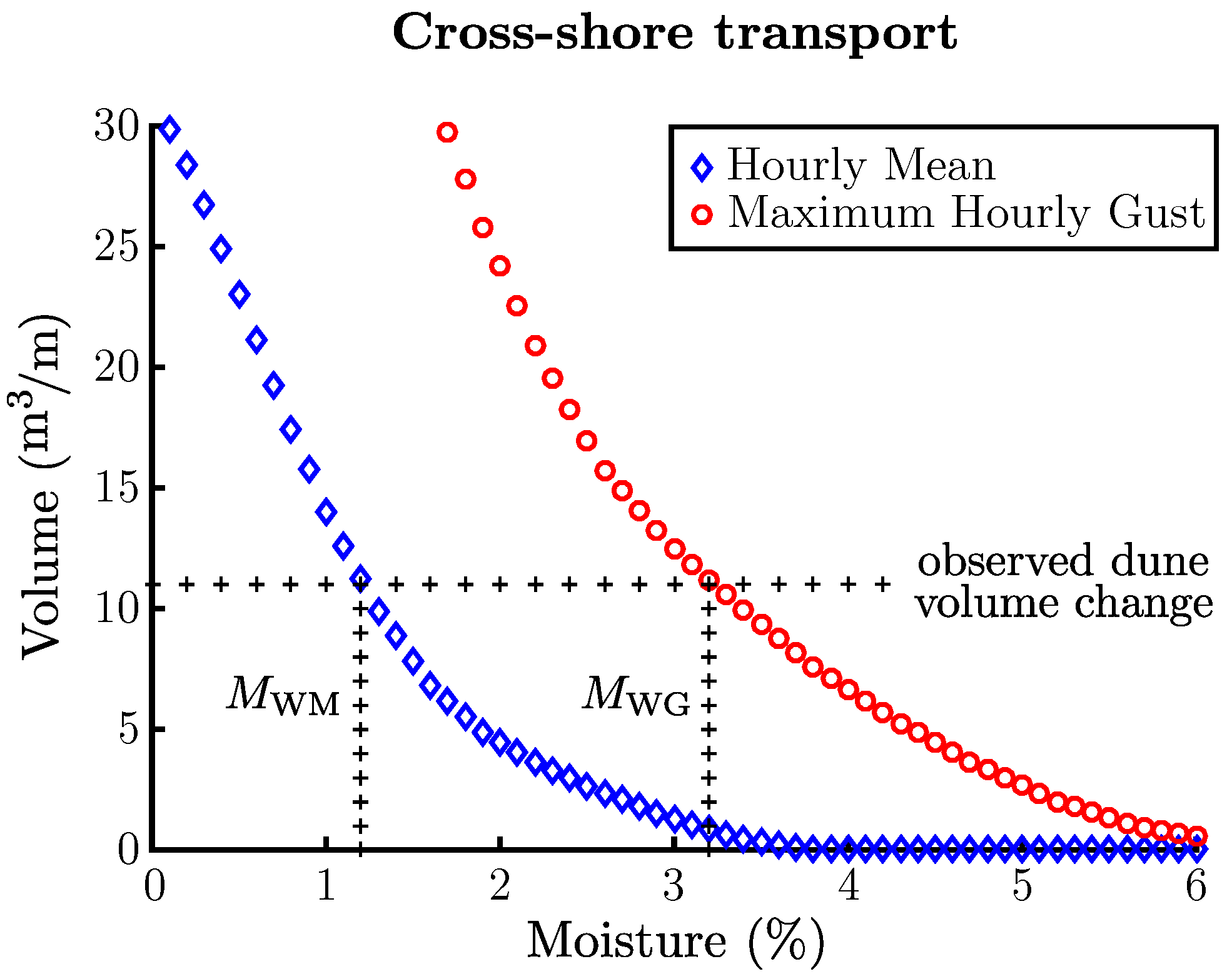
  • The representative moisture content values obtained (1.2% if hourly mean wind speed is used and 3.2% if hourly wind gust is used as input) imply that we need a quite dry beach surface indicating that the main source area for aeolian transport corresponds to the upper part of the intertidal beach, most likely the region between MHTL and SHTL.
  • Due to the high dependency of the representative surface moisture content value on observed dune volume change, the accuracy of the topographic surveys is key to obtain a reliable and representative moisture content.
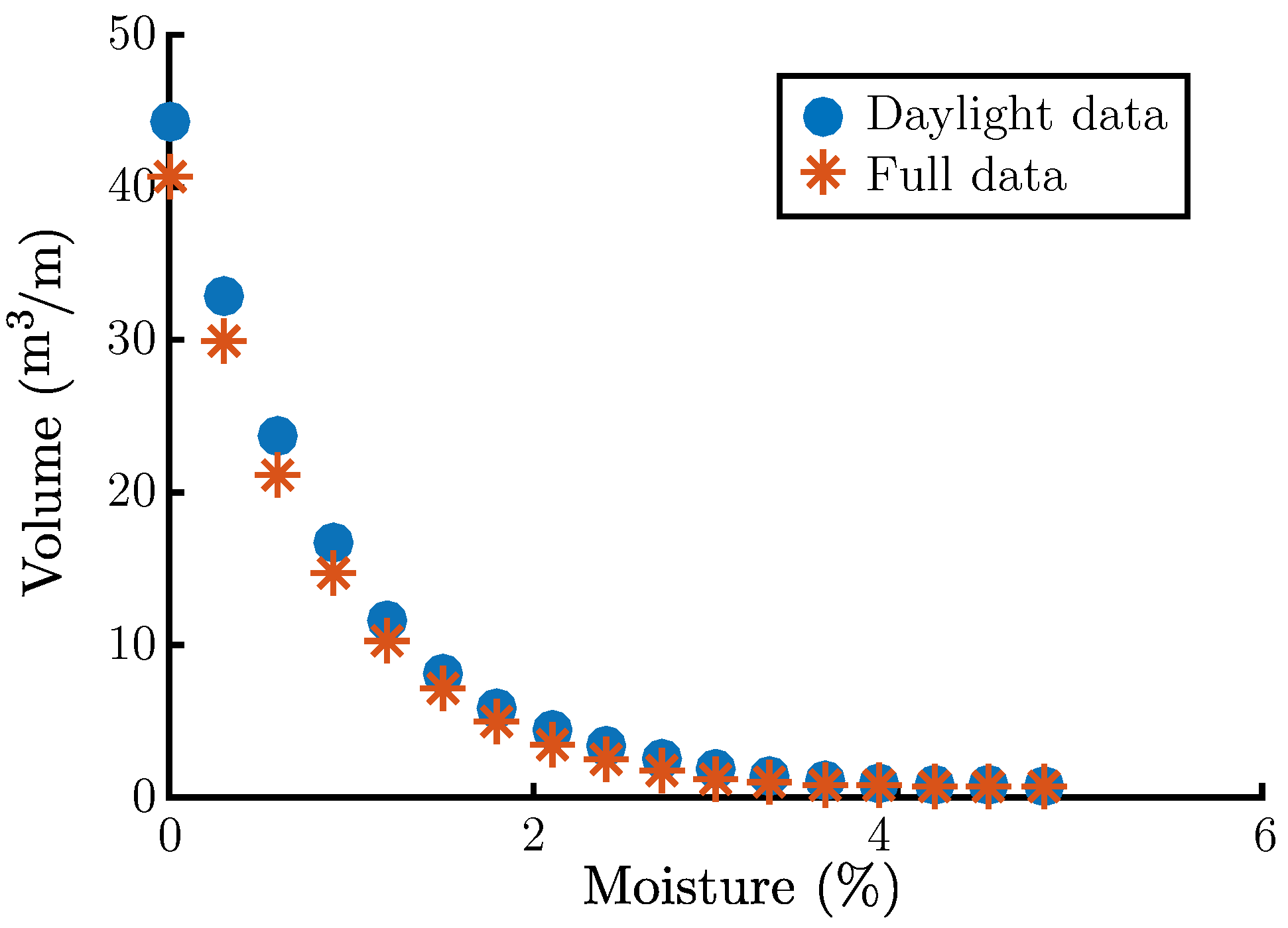
  • The quantification needs the support of the images to detect the days or hours in which transport occurs. Therefore, the availability of video images is an important tool to corroborate the aeolian activity or transport at the beach.

Author Contributions

All authors have conceived, formulated, conducted, and contributed to the work described in this paper. L.D.C. wrote the first draft of the manuscript and all authors contributed to the final text and figures. All authors read and approved the final manuscript.

Funding

This research was funded by Becas-Chile program, attached to the Ministry of Education of Chile.

Acknowledgments

We greatly appreciated the support of Filipe Galiforni Silva (University of Twente) in responding to the LiDAR questions. We thank to Evan B Goldstein (UNC-Chapel Hill) and two anonymous reviewers for their comments that significantly improved this manuscript. The images and LiDAR datasets are owned by Rijkswaterstaat. The weather data are made available by the Royal Netherlands Meteorological Institute (KNMI).

Conflicts of Interest

The authors declare no conflict of interest.

References

  1. Cohn, N.; Ruggiero, P.; Vries, S.; Kaminsky, G.M. New Insights on Coastal Foredune Growth: The Relative Contributions of Marine and Aeolian Processes. Geophys. Res. Lett. 2018, 45, 4965–4973. [Google Scholar] [CrossRef]
  2. Roelvink, D.; Reniers, A.; van Dongeren, A.; van Thiel de Vries, J.; McCall, R.; Lescinski, J. Modelling storm impacts on beaches, dunes and barrier islands. Coast. Eng. 2009, 56, 1133–1152. [Google Scholar] [CrossRef]
  3. Davidson-Arnott, R.; Bauer, B. Aeolian sediment transport on a beach: Thresholds, intermittency, and high frequency variability. Geomorphology 2009, 105, 117–126. [Google Scholar] [CrossRef]
  4. Hanson, H.; Larson, M.; Kraus, N.C. Calculation of beach change under interacting cross-shore and longshore processes. Coast. Eng. 2010, 57, 610–619. [Google Scholar] [CrossRef]
  5. Delgado-Fernandez, I.; Davidson-Arnott, R.; Ollerhead, J. Application of a Remote Sensing Technique to the Study of Coastal Dunes. J. Coast. Res. 2009, 25, 1160–1167. [Google Scholar] [CrossRef]
  6. Delgado-Fernandez, I.; Davidson-Arnott, R. Meso-scale aeolian sediment input to coastal dunes: The nature of aeolian transport events. Geomorphology 2011, 126, 217–232. [Google Scholar] [CrossRef] [Green Version]
  7. Sherman, D.J.; Jackson, D.W.T.; Namikas, S.L.; Wang, J. Wind-blown sand on beaches: An evaluation of models. Geomorphology 1998, 22, 113–133. [Google Scholar] [CrossRef]
  8. Sherman, D.J.; Li, B.; Ellis, J.T.; Farrell, E.J.; Maia, L.P.; Granja, H. Recalibrating aeolian sand transport models. Earth Surf. Proc. Landf. 2013, 38, 169–178. [Google Scholar] [CrossRef]
  9. Bagnold, R.A. The Physics of Blown Sand and Desert Dunes; Dover Publications, Inc.: Mineola, NY, USA, 1941; Second Edition 1954; Reprinted by Dover in 2004. [Google Scholar]
  10. Kawamura, R. Study of Sand Movement by Wind; Report HEL-2-8; Hydraulic Engineering Laboratory, University of California: Berkeley, CA, USA, 1951; Translated from Japanese, 1964. [Google Scholar]
  11. Owen, P.R. Saltation of uniform grains in air. J. Fluid Mech. 1964, 20, 225–242. [Google Scholar] [CrossRef]
  12. Lettau, K.; Lettau, H. Experimental and micrometeorological field studies of dune migration. In Exploring the World’s Driest Climate; Lettau, H.H., Lettau, K., Eds.; Center for Climatic Research, University Wisconsin-Madison: Madison, WI, USA, 1977; pp. 110–147. [Google Scholar]
  13. Durán, O.; Claudin, P.; Andreotti, B. On aeolian transport: Grain-scale interactions, dynamical mechanisms and scaling laws. Aeolian Res. 2011, 3, 243–270. [Google Scholar] [CrossRef]
  14. Kok, J.F.; Parteli, E.J.R.; Michaels, T.I.; Karam, D.B. The physics of wind-blown sand and dust. Rep. Prog. Phys. 2012, 75, 106901. [Google Scholar] [CrossRef] [PubMed]
  15. Hsu, S.A. Computing Eolian Sand Transport from Routine Weather Data. In Proceedings of the 14th Conference on Coastal Engineering, Copenhagen, Denmark, 24–28 July 1974; ASCE: New York, NY, USA, 1974; pp. 1619–1626. [Google Scholar]
  16. Sherman, D.J. An equilibrium relationship for shear velocity and roughness length in aeolian saltation. Geomorphology 1992, 5, 419–431. [Google Scholar] [CrossRef]
  17. Bauer, B.; Davidson-Arnott, R.; Hesp, P.; Namikas, S.; Ollerhead, J.; Walker, I. Aeolian sediment transport on a beach: Surface moisture, wind fetch, and mean transport. Geomorphology 2009, 105, 106–116. [Google Scholar] [CrossRef]
  18. Delgado-Fernandez, I.; Davidson-Arnott, R.; Bauer, B.O.; Walker, I.J.; Ollerhead, J.; Rhew, H. Assessing aeolian beach-surface dynamics using a remote sensing approach. Earth Surf. Proc. Landf. 2012, 37, 1651–1660. [Google Scholar] [CrossRef] [Green Version]
  19. Nield, J.M. Surface moisture-induced feedback in aeolian environments. Geology 2011, 39, 915–918. [Google Scholar] [CrossRef]
  20. Smit, Y.; Ruessink, B.G.; Brakenhoff, L.B.; Donker, J.J. Measuring spatial and temporal variation in surface moisture on a coastal beach with a near-infrared terrestrial laser scanner. Aeolian Res. 2018, 31, 19–27. [Google Scholar] [CrossRef]
  21. Udo, K.; Kuriyama, Y.; Jackson, D.W.T. Observations of wind-blown sand under various meteorological conditions at a beach. J. Geophys. Res. Earth Surf. 2008, 113, F04008. [Google Scholar] [CrossRef]
  22. Hotta, S.; Kubota, S.; Katori, S.; Horikawa, K. Sand Transport by Wind on a Wet Sand Surface. In Proceedings of the 19th Conference on Coastal Engineering, Houston, TX, USA, 3–7 Septembre 1984; ASCE: New York, NY, USA, 1984; pp. 1265–1281. [Google Scholar]
  23. Belly, P.Y. Sand Movement by Wind; CERC Tech. Mem. 1, Addendum III; U.S. Army Corps of Engineers: Washington, DC, USA, 1964; 24p. [Google Scholar]
  24. Dong, Z.; Liu, X.; Wang, X. Wind initiation thresholds of the moistened sands. Geophys. Res. Lett. 2002, 29, 25-1–25-4. [Google Scholar] [CrossRef]
  25. Bauer, B.O.; Davidson-Arnott, R.G.D. A general framework for modeling sediment supply to coastal dunes including wind angle, beach geometry, and fetch effects. Geomorphology 2003, 49, 89–108. [Google Scholar] [CrossRef]
  26. Holman, R.; Stanley, J. The history and technical capabilities of Argus. Coast. Eng. 2007, 54, 477–491. [Google Scholar] [CrossRef]
  27. Smit, M.; Aarninkhof, S.; Wijnberg, K.; Gonzalez, M.; Kingston, K.; Southgate, H.; Ruessink, B.; Holman, R.; Siegle, E.; Davidson, M.; Medina, R. The role of video imagery in predicting daily to monthly coastal evolution. Coast. Eng. 2007, 54, 539–553. [Google Scholar] [CrossRef]
  28. Quartel, S.; Kroon, A.; Ruessink, B. Seasonal accretion and erosion patterns of a microtidal sandy beach. Mar. Geol. 2008, 250, 19–33. [Google Scholar] [CrossRef]
  29. Revollo, N.V.; Delrieux, C.A.; Perillo, G.M. Automatic methodology for mapping of coastal zones in video sequences. Mar. Geol. 2016, 381, 87–101. [Google Scholar] [CrossRef]
  30. Van der Weerd, A.J.; Wijnberg, K.M. Aeolian Sediment Flux Derived from a Natural Sand Trap. J. Coast. Res. 2016, 75, 338–342. [Google Scholar] [CrossRef] [Green Version]
  31. Hage, P.; Ruessink, B.; Donker, J. Determining sand strip characteristics using Argus video monitoring. Aeolian Res. 2018, 33, 1–11. [Google Scholar] [CrossRef]
  32. Williams, I.A.; Wijnberg, K.M.; Hulscher, S.J.M.H. Detection of aeolian transport in coastal images. Aeolian Res. 2018, 35, 47–57. [Google Scholar] [CrossRef]
  33. Van Rijn, L.; Walstra, D.; Grasmeijer, B.; Sutherland, J.; Pan, S.; Sierra, J. The predictability of cross-shore bed evolution of sandy beaches at the time scale of storms and seasons using process-based Profile models. Coast. Eng. 2003, 47, 295–327. [Google Scholar] [CrossRef]
  34. Bakker, M.A.J.; van Heteren, S.; Vonhögen, L.M.; van der Spek, A.J.F.; van der Valk, B. Recent Coastal Dune Development: Effects of Sand Nourishments. J. Coast. Res. 2012, 28, 587–601. [Google Scholar] [CrossRef]
  35. De Winter, R.; Gongriep, F.; Ruessink, B. Observations and modeling of alongshore variability in dune erosion at Egmond aan Zee, the Netherlands. Coast. Eng. 2015, 99, 167–175. [Google Scholar] [CrossRef]
  36. Uunk, L.; Wijnberg, K.; Morelissen, R. Automated mapping of the intertidal beach bathymetry from video images. Coast. Eng. 2010, 57, 461–469. [Google Scholar] [CrossRef]
  37. De Winter, W.; van Dam, D.; Delbecque, N.; Verdoodt, A.; Ruessink, B.; Sterk, G. Measuring high spatiotemporal variability in saltation intensity using a low-cost Saltation Detection System: Wind tunnel and field experiments. Aeolian Res. 2018, 31, 72–81. [Google Scholar] [CrossRef]
  38. Lynch, K.; Jackson, D.W.T.; Cooper, J.A.G. The fetch effect on aeolian sediment transport on a sandy beach: A case study from Magilligan Strand, Northern Ireland. Earth Surf. Proc. Landf. 2016, 41, 1129–1135. [Google Scholar] [CrossRef]
  39. Bochev-van der Burgh, L.M.; Wijnberg, K.M.; Hulscher, S.J.M.H. Decadal-scale morphologic variability of managed coastal dunes. Coast. Eng. 2011, 58, 927–936. [Google Scholar] [CrossRef]
  40. Ruessink, B.; Arens, S.; Kuipers, M.; Donker, J. Coastal dune dynamics in response to excavated foredune notches. Aeolian Res. 2018, 31, 3–17. [Google Scholar] [CrossRef]
  41. Rijkswaterstaat. Kwaliteitsdocument laseraltimetrie. Deel 2: Projectgebied Kust 2012 Perceel 1; Data-ICT Dienst: Utrecht, The Netherlands, 2012. (In Dutch) [Google Scholar]
  42. Bauer, B.O.; Hesp, P.A.; Walker, I.J.; Davidson-Arnott, R.G. Sediment transport (dis)continuity across a beach-dune profile ing an offshore wind event. Geomorphology 2015, 245, 135–148. [Google Scholar] [CrossRef]
  43. Nordstrom, K.F.; Jackson, N.L. Offshore aeolian sediment transport across a human-modified foredune. Earth Surf. Proc. Landf. 2017, 43, 195–201. [Google Scholar] [CrossRef] [Green Version]
  44. Reim, E. Annual Aeolian Sediment Transport from the Intertidal Beach. Master’s Thesis, University of Twente, Enschede, The Netherlands, 2013. [Google Scholar]
  45. Kim, S.W.; Yun, K.; Yi, K.M.; Kim, S.J.; Choi, J.Y. Detection of Moving Objects with a Moving Camera Using Non-panoramic Background Model. Mach. Vis. Appl. 2013, 24, 1015–1028. [Google Scholar] [CrossRef]
  46. Bagnold, R.A. The Movement of Desert Sand. Proc. R. Soc. A 1936, 157, 594–620. [Google Scholar] [CrossRef]
  47. Bauer, B.O.; Davidson-Arnott, R.G.D.; Walker, I.J.; Hesp, P.A.; Ollerhead, J. Wind direction and complex sediment transport response across a beach-dune system. Earth Surf. Proc. Landf. 2012, 37, 1661–1677. [Google Scholar] [CrossRef]
  48. Azizov, A. Influence of soil moisture on the resistance of soil to wind erosion. Sov. Soil Sci. 1977, 9, 105–108. [Google Scholar]
  49. Davidson-Arnott, R.G.D.; Bauer, B.O.; Walker, I.J.; Hesp, P.A.; Ollerhead, J.; Delgado-Fernandez, I. Instantaneous and mean aeolian sediment transport rate on beaches: an intercomparison of measurements from two sensor types. J. Coast. Res. 2009, 56, 297–301. [Google Scholar]
  50. Davidson-Arnott, R.G.D.; Yang, Y.; Ollerhead, J.; Hesp, P.A.; Walker, I.J. The effects of surface moisture on aeolian sediment transport threshold and mass flux on a beach. Earth Surf. Proc. Landf. 2008, 33, 55–74. [Google Scholar] [CrossRef]
  51. Stive, M.J.; de Schipper, M.A.; Luijendijk, A.P.; Aarninkhof, S.G.; van Gelder-Maas, C.; van Thiel de Vries, J.S.; de Vries, S.; Henriquez, M.; Marx, S.; Ranasinghe, R. A New Alternative to Saving Our Beaches from Sea-Level Rise: The Sand Engine. J. Coast. Res. 2013, 29, 1001–1008. [Google Scholar] [CrossRef]
  52. Silva, F.G.; Wijnberg, K.M.; de Groot, A.V.; Hulscher, S.J.M.H. The influence of groundwater depth on coastal dune development at sand flats close to inlets. Ocean Dyn. 2018, 68, 885–897. [Google Scholar] [CrossRef]
  53. Montreuil, A.L.; Chen, M.; Brand, E.; Strypsteen, G.; Rauwoens, P.; Vandenbulcke, A.; De Wulf, A.; Dan, S.; Verwaest, T. Dynamics of Surface Moisture Content on a Macro-tidal Beach. J. Coast. Res. 2018, 85, 206–210. [Google Scholar] [CrossRef]
  54. Namikas, S.; Edwards, B.; Bitton, M.; Booth, J.; Zhu, Y. Temporal and spatial variabilities in the surface moisture content of a fine-grained beach. Geomorphology 2010, 114, 303–310. [Google Scholar] [CrossRef]
  55. Poortinga, A.; van Rheenen, H.; Ellis, J.T.; Sherman, D.J. Measuring aeolian sand transport using acoustic sensors. Aeolian Res. 2015, 16, 143–151. [Google Scholar] [CrossRef]
  56. Rijkswaterstaat. Kwaliteitsdocument Laseraltimetrie: Resultaten Controles Kust; Combinatie Hansa Luftbild/ TopScan in Opdracht van Rijkswaterstaat: Utrecht, The Netherlands, 2015. (In Dutch) [Google Scholar]
  57. Jensen, S.G.; Aagaard, T.; Baldock, T.E.; Kroon, A.; Hughes, M. Berm formation and dynamics on a gently sloping beach; the effect of water level and swash overtopping. Earth Surf. Proc. Landf. 2009, 34, 1533–1546. [Google Scholar] [CrossRef]
  58. Aarninkhof, S.G.; Turner, I.L.; Dronkers, T.D.; Caljouw, M.; Nipius, L. A video-based technique for mapping intertidal beach bathymetry. Coast. Eng. 2003, 49, 275–289. [Google Scholar] [CrossRef]
Figure 1. Conceptual model for Aeolian (red arrows) and Hydrodynamics (blue arrows) accretion sand exchange across a beach.
Jmse 06 00127 g001
Figure 2. Effect of the wind direction in the transport, or cosine effect, explained in an Argus image. Where α is the angle formed by the wind direction and the perpendicular projection from the dune foot to the shoreline.
Jmse 06 00127 g002
Figure 3. Study area and its location in the Dutch coast.
Jmse 06 00127 g003
Figure 4. Argus station-Coast3D tower-at Egmond Beach.
Jmse 06 00127 g004
Figure 5. Annual dune volume variation above 3 m+NAP at Egmond Beach. The red dot represents the volume increase during the year 2009 (March 2009–March 2010). For the years 2000 and 2002 there are no data available and therefore, no volume change is plotted for the years that depend on these measurements, i.e., 1999, 2000, 2001 and 2002.
Jmse 06 00127 g005
Figure 6. Change in elevation (m) at the beach and dunes area around the Coast 3D tower, between the years 2010 and 2009, obtained from the LiDAR data. The black line represents the contour line at 3 m+NAP and the gray line is the contour for 0 m+NAP. The location of the Argus Tower is represented by a black cross.
Jmse 06 00127 g006
Figure 7. Aeolian sand transport observed from 6 chronological snapshots at Egmond Beach (Argus Images, 19 October 2009. (1) 9:00 h–(2) 10:00 h–(3) 11:00 h–(4) 12:00 h–(5) 13:00 h–(6) 14:00 h). The red-dashed line represents the spring high tide line and the enclosed white-dashed area serves as a guide to observe the transport in the images. The average wind speed during these hours ranged between 9 and 12 m/s, and the wind direction varied between 190°–220°, being alongshore at 9:00 h and southwest wind at 14:00 h. No rain was measured during this period.
Jmse 06 00127 g007
Figure 8. (a) Color and (b) grayscale Argus image of 19 October 2009 at 10:00 a.m. (c) Pixel Intensity plot of grayscale images of a whole day (8:00 to 16:00 h) to detect aeolian sand transport. The pixel area shown in the intensity plot corresponds to the line at pixel 1200 in the horizontal axis, and between pixels 600 to 1000 in the vertical axis, which is located inside of the white rectangular area, in the grayscale image (b).
Jmse 06 00127 g008
Figure 9. Hourly average wind direction distribution and frequency (red numbers) during the period March 2009–March 2010.
Jmse 06 00127 g009
Figure 10. Hourly average wind speed values during the period March 2009–March 2010 according their wind direction, for wind speeds larger than the observed wind speed threshold. (a) 180°–240°, (b) 240°–300° and (c) 300°–360°.
Jmse 06 00127 g010
Figure 11. (a) Predicted Total and (b) Cross-Shore transported volume of sand ( m 3 /m), due to aeolian sand transport from the intertidal beach at Egmond Beach for the period March 2009–March 2010, for several surface moisture content values. We calculated the transport using the Kawamura equation (Equation (2)) and considering the moisture effect in the threshold shear velocity ( U t m ) (Equation (4)). The input data correspond to the hourly mean wind speed and gust wind speed, for the time in which sand transport was observed and the proportionality factor ( P = 3 ) to obtain annual amounts.
Jmse 06 00127 g011
Figure 12. Calculated cross-shore sand transport from the intertidal beach as a function of moisture content (M), for the period 18 March 2009–11 March 2010. Moisture values M W M and M W G correspond to the moisture values for which calculated transport matches observed dune volume change (during the same period) for hourly wind mean and hourly wind gust respectively.
Jmse 06 00127 g012
Figure 13. Transport quantification (dune volume increase) for various surface moisture content, for (a) hourly mean and (b) gust wind speed for the period 18 March 2009–11 March 2010. Volume was calculated using: (1) Equation (2), considering images, i.e., hours of transport occurrence and wind speed (red triangles) and wind speed data (blue circles); (2) Equation (6), considering wind and water levels (red squares); wind and rain (yellow crosses); and wind, rain and water levels (purple stars). The red triangles for hourly mean and gust wind speed correspond to the blue diamonds and red circles in Figure 12 respectively.
Jmse 06 00127 g013
Figure 14. Comparison of volumes for different moisture values, obtained from the full wind data set and during daylight data (8:00–16:00), for the period 18 March 2009–11 March 2010.
Jmse 06 00127 g014
Figure 15. (a) Comparison of volume increase (calculated and measured) for years without storm surges, 2008, 2009, 2010 and 2012. The maximum water level during these years was lower than 2.0 m. The blue dots represent the volume calculated according Equation (6), considering hourly average wind speed data and a surface moisture content ( M W M ) equal to 1.2%. The red dots represent the volumes transported during the same years, but the only data considered corresponds to hourly average wind speed, i.e., M = 0%. The dashed line represents a 1 to 1 slope line. (b) A zoom-in of the calculations using a moisture content of 1.2%. The error bars represent the volumes obtained for moisture contents of 1.0% and 1.5% and the error related to the LiDAR measurements.
Jmse 06 00127 g015
Figure 16. Cumulative distribution of water levels (a) and wind speeds (b) during hours in which transport or no transport was observed in the images, when U U Threshold = 7 m/s considering onshore wind conditions and its relationship with the presence or absence of rain during the same hour.
Jmse 06 00127 g016
Table 1. Constant C from Dong et al. [24] that relates threshold shear velocity and moisture content according to the mean grain size.
Grain Size (μm)C
45–541.59
54–771.85
77–902.46
90–1001.66
100–1352.51
135–1502.05
150–2002.75
200–2501.59
250–4001.87
400–5002.15
Table 2. Amount of hours in which transport or no transport was observed in the images, when  U U Threshold , and its relationship with the presence or absence of rain during the same hour. Where U Threshold = 5 m/s corresponds to the minimum hourly wind speed at which transport was observed in the images.
Rain
YesNo
Transport
Images
Yes113615
No2241456
Table 3. Years in which the aggregated transport formula was evaluated with their respective LiDAR survey dates and the maximum water level per period.
YearLidar Survey DatesMax Water Level
20089 April 2008–18 March 20091.85 m
200918 March 2009–11 March 20101.92 m
201011 March 2010–27 January 20111.79 m
20121 February 2012–14 January 20131.71 m
Table 4. Volume change during years in which maximum water level was lower than 2.0 m. The  volumes correspond to those obtained from LiDAR data and to the calculated ones with Equation  (6), considering hourly average wind speed data and a representative moisture content equal to 1.2%, except for the last column in which moisture was not considered and hourly average wind speed is the only data considered. The heading of each column represents the data considered to calculate the respective volume. Volumes in m 3 /m.
Year L idar W ind W ind + R ain W ind + W Level W ind + R ain + W Level W ind ( 0 % )
200818.814.26.313.46.357.6
200911.218.011.117.811.063.4
201012.611.58.09.66.244.4
201215.615.19.915.19.960.0
Table 5. Volume change during years in which maximum water level was lower than 2.0 m. The  volumes correspond to those obtained from LiDAR data and to the calculated ones with Equation  (6), considering hourly maximum wind speed (gust) data and a representative moisture content equal to 3.2%, except for the last column in which moisture was not considered and wind gust is the only data considered. The heading of each column represents the data considered to calculate the respective volume. Volumes in m 3 /m.
Year L idar G ust G ust + R ain G ust + W Level G ust + R ain + W Level G ust (0%)
200818.814.74.712.84.7131.1
200911.218.810.018.89.9146.9
201012.68.65.26.22.8103.6
201215.619.311.419.311.4149.6
Table 6. Amount of hours in which transport or no transport was observed in the images, when U U Threshold considering onshore wind conditions and its relationship with the presence or absence of rain during the same hour. Where U Threshold Onshore = 7 m/s corresponds to the minimum hourly wind speed at which transport was observed in the images.
Rain
YesNo
Transport
Images
Yes84422
No93524
Table 7. Average water level (m above NAP) in which transport or no transport was observed in the images, when U U Threshold considering onshore wind conditions and its relationship with the presence or absence of rain during the same hour. Where U Threshold Onshore = 7 m/s corresponds to the minimum hourly wind speed at which transport was observed in the images.
Rain
YesNo
Transport
Images
Yes0.070.17
No0.260.24
Table 8. Volume change during years in which maximum water level was lower than 2.0 m. The  volumes correspond to those obtained from LiDAR data (based on considerations about measurement error) and to the calculated ones with Equation (6), considering hourly average wind speed data and a representative moisture content equal to 1%. The heading of each column represents the data considered to calculate the respective volume. Volumes in m 3 /m.
Year L idar W ind W ind + R ain W ind + W Level W ind + R ain + W Level
200815.818.010.117.110.1
200914.222.715.722.415.5
20109.614.811.312.89.4
201212.6–18.619.014.119.014.1

