A Sensitivity Analysis of the Wind Forcing Effect on the Accuracy of Large-Wave Hindcasting


Pacific Northwest National Laboratory, 1100 Dexter Avenue North, Suite 500, Seattle, WA 98109, USA
*
Author to whom correspondence should be addressed.
J. Mar. Sci. Eng. 2018, 6(4), 139; https://doi.org/10.3390/jmse6040139
Submission received: 29 September 2018
/
Revised: 2 November 2018
/
Accepted: 5 November 2018
/
Published: 14 November 2018
(This article belongs to the Special Issue Selected Papers from the 15th Estuarine and Coastal Modeling Conference)
Abstract
:Deployment of wave energy converters (WECs) relies on consistent and accurate wave resource characterization, which is typically achieved through numerical modeling using deterministic wave models. The accurate predictions of large-wave events are critical to the success of wave resource characterization because of the risk on WEC installation, maintenance, and damage caused by extreme sea states. Because wind forcing is the primary driver of wave models, the quality of wind data plays an important role in the accuracy of wave predictions. This study evaluates the sensitivity of large-wave prediction to different wind-forcing products, and identifies a feasible approach to improve wave model results through improved wind forcing. Using a multi-level nested-grid modeling approach, we perform a series of sensitivity tests at four representative National Data Buoy Center buoy locations on the U.S. East and West Coasts. The selected wind-forcing products include the Climate Forecast System Reanalysis global wind product and North American Regional Reanalysis regional wind product as well as the observed wind at the buoys. Sensitivity test results indicate a consistent improvement in model predictions for the large-wave events (e.g., >90th percentile of significant wave height) at all buoys when observed-wind data were used to drive the wave model simulations.
1. Introduction
The accuracy of wave models in simulating wave climates is critical to the success of wave energy development, especially in nearshore regions where wave energy development is most likely to occur. As recommended by the International Electrotechnical Commission Technical Specifications (IEC TS) [1], the development of wave energy projects relies on consistent and accurate wave resource characterization, which is typically achieved through high-resolution wave modeling at the project sites. One gap in this modeling effort is the accurate prediction of large-wave events, e.g., the waves that account for the 90th percentile of the significant wave height and are usually produced by storms, such as tropical and extratropical cyclones.
In many wave modeling studies, large waves have been consistently underpredicted compared to measurements at buoys, especially under extreme weather conditions, such as hurricanes and typhoons [2,3]. For instance, Pan et al. [3] evaluated the performance of an operational wind wave forecasting system in Taiwan, and found the averaged peak wave heights were underestimated during typhoon events. By using multiple wind inputs to model a cyclone event, a regional wave model used near Newport, Oregon underestimated the large waves for all simulations [4]. A global wave model using the Climate Forecast System Reanalysis (CFSR) global wind product for the long-term wave hindcast also produced the largest errors during winter months and large-wave events [5]. In our earlier studies [6,7], we successfully applied two third-generation spectral wave models, WaveWatch III (WWIII) [8,9] and the Unstructured version of Simulate Wave Near Shore (UnSWAN) [10], to simulate wave climates on the U.S. West Coast based on the National Oceanic and Atmospheric Administration’s (NOAA’s) National Centers for Environmental Protection (NCEP) global CFSR wind product [11]. Overall, the model-data comparisons showed satisfactory model performance with correlation coefficients (R) greater than 0.9 for both the omnidirectional power and significant wave height at nearly all validation National Data Buoy Center (NDBC) buoys. However, the results also indicated that, especially for the nearshore buoys, both models tend to underpredict the significant wave height and wave power during large-wave events [6,7].
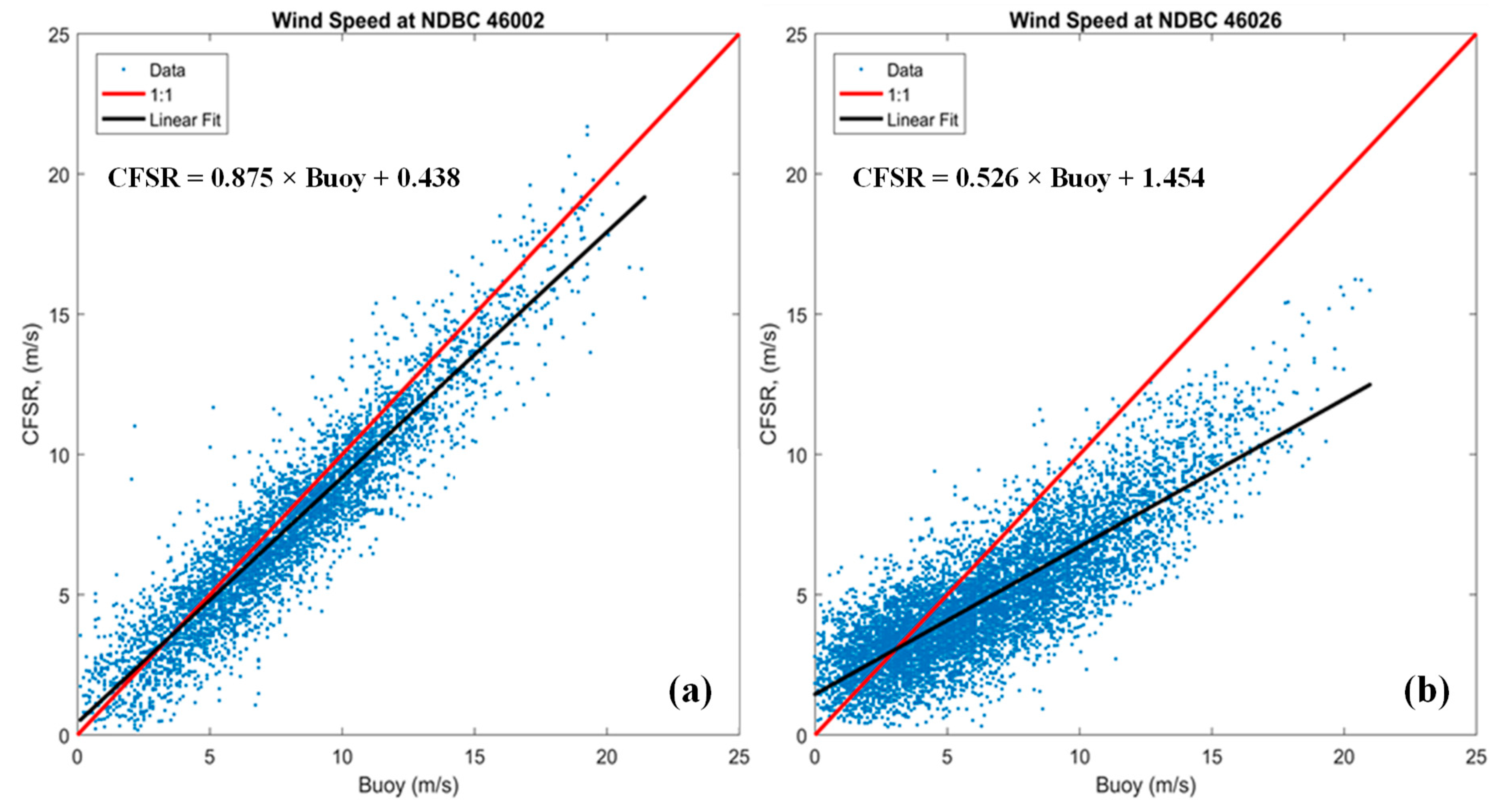
As pointed out by other similar studies, the underestimation of large waves could be partially constrained by the accuracy of wind forcing during the storm events, especially of those operational global wind-model products [2,3,4,12]. A quick comparison of the CFSR wind with observed wind at NDBC buoys also confirmed that the discrepancy in wave predictions appears to be consistent with that in the wind forcing. Figure 1 shows the comparisons between CFSR wind and observed buoy wind at two buoys in the northeast Pacific Ocean—an offshore buoy, NDBC 46002 (~270 nautical miles offshore), and a nearshore buoy, NDBC 46026 (18 nautical miles from San Francisco, CA, USA). The comparisons indicate that the CFSR wind product generally performs much better in the open ocean than in the nearshore regions. At the nearshore Buoy 46026, the CFSR wind product substantially underestimates high wind (i.e., wind speed greater than 5 m/s).
Because wind forcing is the primary driver for wave models, its quality plays a critical role in determining the accuracy of wave predictions. Thus, it is necessary to investigate whether wave model results can be improved by using more accurate wind-forcing products, such as observed wind. This paper presents a study to evaluate the sensitivity of wave models to different wind-forcing products and to identify a feasible approach for improving wave model results through improved wind forcing, with a special focus on large-wave predictions. Improving large-wave prediction not only provides important siting information for WEC development, but also reduces associated maritime risk, such as damage to coastal zones and coastal infrastructure.
2. Methods
2.1. Selection of Study Sites
To conduct the wind-sensitivity tests, we selected four representative NDBC buoys as the study sites and reviewed available wind-model products. A number of NDBC buoys in U.S. West and East Coasts were evaluated, and four representative buoys were finally selected based on the combination of the following criteria:
- Availability of high-quality wave data for wave model validation and wind data for evaluation of the quality of the modeled wind products;
- high wave energy resource and proximity to shore; and
- representativeness of regional distribution.
In general, the number of NDBC buoys that have high-quality, concurrent wave and wind observations is limited. We reviewed all nearshore NDBC buoys on the U.S. West and East Coasts and selected four study sites based on the criteria listed above. Of the four sites, two are located on the West Coast and two on the East Coast (Figure 2). Specifically:
- NDBC 46050, Stonewall Bank, Oregon, USA. This site was selected because of its high wave resource potential and high-quality wave and wind data, as well as its intermediate water depth and proximity to shore (20 nautical miles from Newport, OR, USA). It is also adjacent to the North Energy Test Site, managed by the Pacific Marine Energy Center, and has been studied extensively [6,13,14,15,16].
- NBDC 46026, San Francisco, California, USA. This site was selected to represent the wind and wave characteristics of the California coast. NDBC 46026 is located 18 nautical miles from San Francisco and has long-term wind and wave records dating back to 1982. Unlike the narrow continental shelf off the Oregon and northern California coasts, the continental shelf off San Francisco Bay is relatively broad and NDBC 46026 is at a shallow-water depth of 53 m. This study site will provide insight into the effect of wind forcing on shallow-water wave modeling on the West Coast.
- NDBC 44013, Boston, Massachusetts, USA. Although wave resources on the East Coast are smaller than those on the West Coast, the New England region still has a significant amount of wave energy, according to the Electric Power Research Institute, Inc. (Palo Alto, CA, USA) [17]. Based on a recent analysis by the National Renewable Energy Laboratory (NREL) [18], the Massachusetts coast is among the highest-ranked sites in terms of wave resources and market potential. Therefore, the Boston Harbor and coast were selected for their relatively high wave resource as being representative of the New England region. NDBC 44013 is located 16 nautical miles offshore at a water depth of 64.5 m. It also has good quality, long-term observed wave and wind data dating back to 1984.
- NDBC 41025, Diamond Shoals, NC, USA. North Carolina’s coast is the only region identified as a high-resource and -market potential site south of the New England coast in NREL’s study [18]. NDBC 41025 is located near the edge of the continental shelf break and the Hatteras Canyon. It is located at a water depth of 68.3 m and about 16 nautical miles from Cape Hatteras. The North Carolina coast is also regularly subjected to the threat of tropical cyclones. Therefore, this study site will provide important information regarding the effect of extreme wind events on the accuracy of model simulations for large waves.
2.2. Review of Wind Products
Many community atmospheric modeling products are publicly available for use to drive ocean circulation and surface wave models. Among them, the following six global and regional atmospheric products are the most common ones currently being used by the ocean modeling community (Table 1):
- NOAA NCEP’s CFSR. Since 2011, the CFSR was upgraded to CFS Version 2 (CFSv2);
- NOAA NCEP’s Global Forecast System (GFS);
- European Centre for Medium-Range Weather Forecasts (ECMWF);
- Japan Meteorological Agency’s Japanese ReAnalysis (JRA);
- NCEP’s North American Regional Reanalysis (NARR); and
- NCEP’s North American Mesoscale Forecast System (NAM).
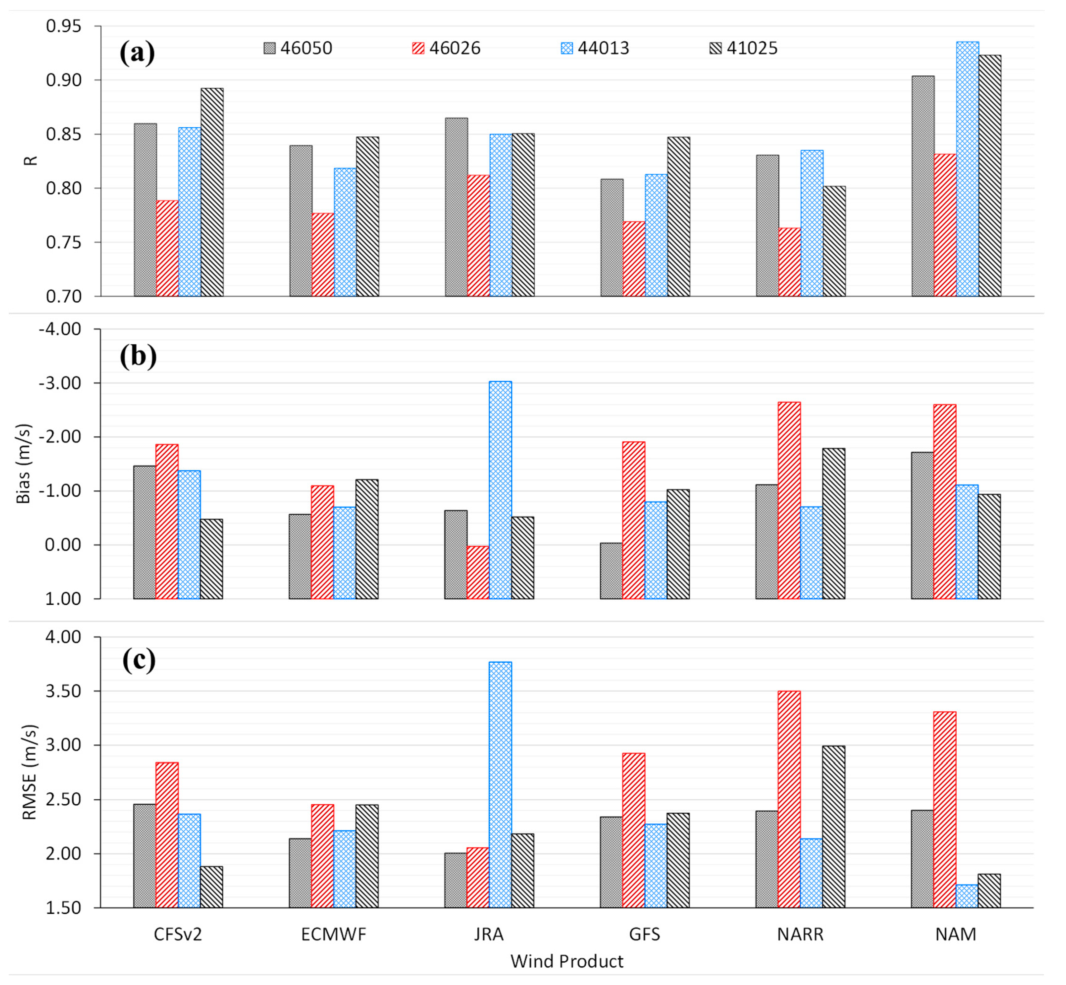
The spatial and temporal coverages and resolutions of these six wind products are listed in Table 1. Due to time and resource constraints, a subset of wind products was further selected to drive wave simulations for the wind-sensitivity analysis after a comparative review of their performance against the observed wind and their temporal and spatial resolutions. Figure 3 shows the performance statistics of wind speed for the full year of 2016. As indicated by the negative bias at nearly all buoys, most wind-model products tend to underpredict wind speed in comparison to buoy observations. Overall, the performance statistics for all four global products are comparable. For the two regional products, NAM performs better than NARR, especially when judged by the correlation coefficient (R) and root mean square error (RMSE) parameters. The comparisons also indicate that all model products perform the worst at NDBC 46026, the shallow-water buoy off the coast of San Francisco Bay.
Because CFSR/CFSv2 wind has a much higher temporal resolution (hourly) than the other three global products (three-hourly) and has been widely used for wave energy resource modeling on the U.S. coasts, we decided to use the global wind product from CFSR/CFSv2 for wind-sensitivity analysis. Due to time and resource constraints, other global wind products (ECMWF, JRA, and GFS) were not considered in this study. For the regional wind product, because the six-hourly resolution of NAM is far below the IEC TS criterion for temporal resolution, we chose to use NARR for this study.
2.3. Model Configuration
Following the path of previous wave modeling work [6,7], we employed a similar multi-level nested-grid modeling approach in this study. This approach combines the strength of the WWIII and UnSWAN models in simulating waves in open oceans with structured grids and those in nearshore regions with flexible, unstructured grids. WWIII and SWAN are among the most widely used third-generation, phase-averaging spectral wave models. WWIII has been maintained and used by NOAA’s NCEP for operational ocean wave forecasts from global to regional scales [9]. SWAN is developed at Delft University of Technology, and computes random, short-crested, wind-generated waves in coastal regions and inland waters [10]. The unstructured version of SWAN is especially suitable for simulating waves in nearshore regions with complex geometry. Specifically, we generated fine-resolution (from ~100 m to several kilometers) UnSWAN model grids around the four NDBC buoys (Figure 2) to serve as the local-level model domains. The model grid bathymetry was interpolated from NOAA’s three arc-second Coastal Relief Model and available high-resolution (1/3 arc-second) tsunami bathymetry data sets. In addition, the three nested structured-grid WWIII model domains provided wave open boundaries for the UnSWAN domains. The WWIII model configuration was based on NOAA/NCEP’s multi-resolution, nested WWIII model package [8], which includes a global model domain of 30′ resolution and two finer levels (10′ and 4′) of nesting domains for the U.S. West and East Coasts (Figure 2). Hourly spectral output from the 4-arc minute WWIII model domains provided the open boundary forcing at each open boundary node of the UnSWAN domains.
The model configuration for UnSWAN simulations was specified in the same way as that specified by Wu et al. [7]; i.e., the model uses 24 direction bins and 29 spectral frequency bins with a logarithmic increment factor of 1.1 covering the frequency range from 0.035 Hz to 0.505 Hz. This spectral resolution meets the minimum requirements specified by the IEC TS; i.e., a minimum of 25 frequency components and 24 to 48 directional components, and a frequency range covering at least 0.04 to 0.5 Hz. The WWIII model was configured in a way similar to that described by Chawla et al. [8], except that the ST2 source term package was replaced with the ST4 source term package, and the spectral resolution was changed to 29 bins, matching those used by the UnSWAN model. The ST4 physics package consists of new parameterizations for swell, wave breaking, and short-wave dissipations of wind-generated waves, which are consistent under a wide range of conditions and at scales from the global ocean to coastal regions [19]. The previous study demonstrated that the ST4 package consistently produced more accurate model results for unidirectional power density and significant wave height parameters [6]. The model versions used in this study are v41.20 for UnSWAN and v5.08 for WWIII.
2.4. Model Simulations
Five sensitivity runs (Table 2) were conducted, including the baseline-condition simulations for the WWIII and UnSWAN models (Runs 1 and 2, respectively), in which both models were forced by the CFSR wind. The configuration of the baseline condition was also consistent with that in the previous studies [6,7]. Because the primary focus of this study was to evaluate whether better wind forcing, especially with the most accurate observational wind data at the buoys, can improve wave results, a sensitivity run (Run 4) with observed wind forcing was conducted for all UnSWAN domains. Meanwhile, a sensitivity run (Run 3) without wind was conducted to examine the effect of wind forcing on wave simulations at the local-level UnSWAN domains. Lastly, to evaluate whether the regional wind product with a finer spatial resolution could improve wave model results, we conducted a sensitivity run (Run 5) by replacing CFSR wind with NARR wind for the 4′ WWIII model domains using the nested-grid WWIII model. To be consistent with previous studies [6,7], we decided to use the same calendar year of 2009 as the simulation period in this study.
A number of statistics parameters (e.g., R, RMSE) have been widely used for assessing numerical model performance [6,7,15,16] and quantifying the discrepancies between model predictions and observations. These metrics represent an average estimate of the difference between predicted values and measured ones over a defined period of simulation. In this study, we calculated the same metrics for all model simulations by primarily focusing on significant wave height—the most representative parameter indicating the performance of wave models. The performance metrics include the aforementioned R, bias, RMSE, percentage error (PE), scatter index (SI), and percentage bias. The equations are provided in the Appendix A at the end of this paper.
3. Results and Discussion
3.1. Baseline Condition with CFSR Wind
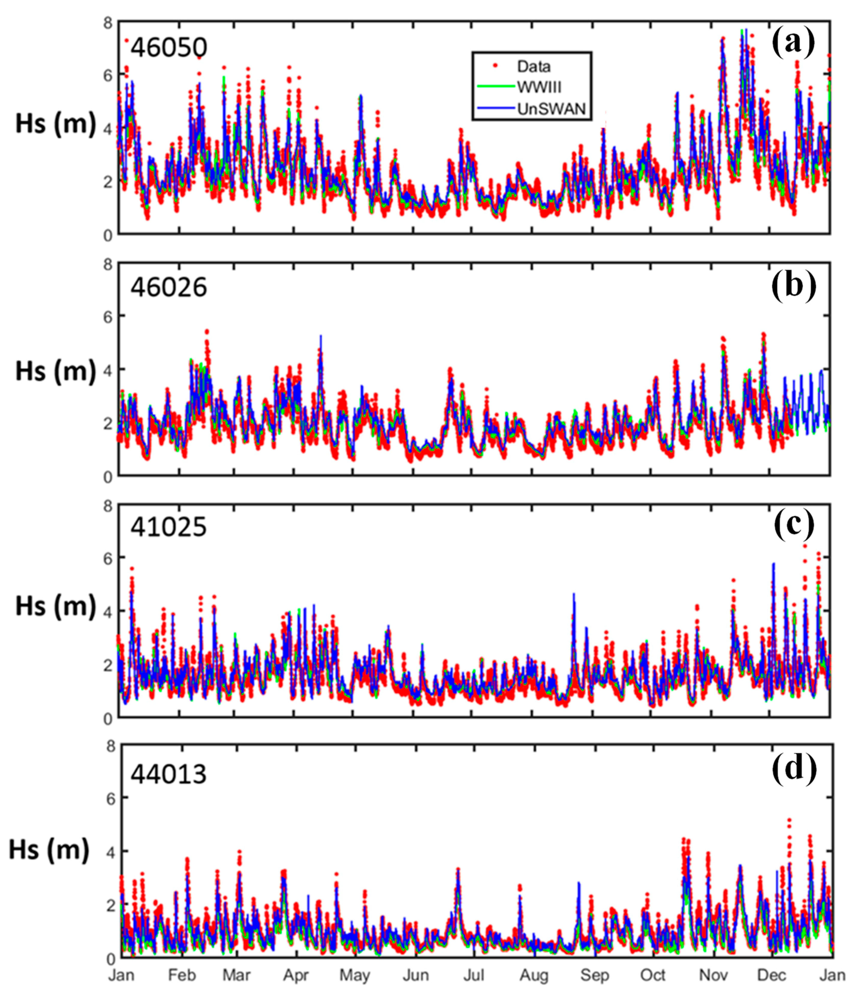
The model results for each sensitivity simulation were analyzed and compared to buoy observations. Figure 4 shows the time series comparisons between model predictions and field observations of significant wave height at all four buoys. The performance metrics are presented in Table 3. Overall, both WWIII and UnSWAN predictions compared very well with the data; the predictions had a correlation coefficient greater than 0.9 at most stations. The models were able to capture the seasonal variability and most individual wave events. WWIII appears to perform slightly better than UnSWAN, which is consistent with previous findings [6]. Both WWIII and UnSWAN show a positive bias at most buoys except for NDBC 44013, and UnSWAN predictions are even more positively biased than the WWIII predictions.
3.2. Simulation without Wind Forcing
To evaluate the wind effect, we analyzed and compared the results of significant wave height for the no-wind sensitivity run with those of the baseline condition. The results (Figure 5) show the one-month time series comparisons in summer and winter, respectively. Obviously, without wind forcing for the UnSWAN domain, the model results became substantially worse compared to those in the baseline condition forced by the CFSR wind. For instance, at Buoy 46026, the major wave events around 20 June 2009 were largely under predicted (Figure 5), suggesting local wind plays an important role in wave generation, and thus must be considered.
3.3. Simulation with Observed Wind
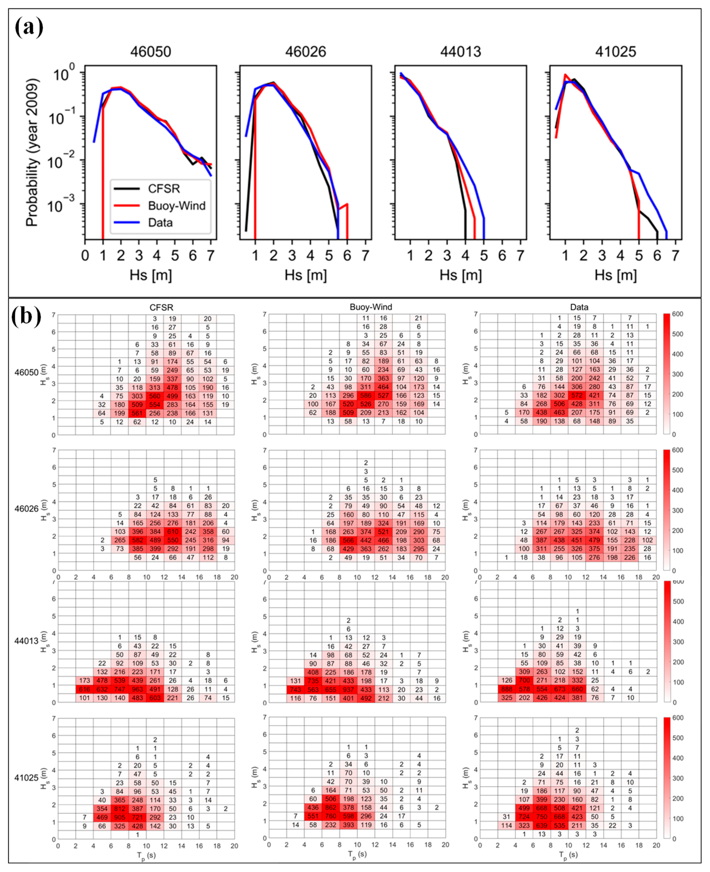
It is important to see if observed wind forcing can improve UnSWAN model results, especially for the large-wave events. Figure 6a shows the probability distribution comparisons of significant wave height between the baseline condition and the sensitivity run with observed wind. Overall, the results are comparable to those of the baseline condition. The model performance was improved for large waves with buoy-wind, especially at the two nearshore buoys, 46026 and 44013, e.g., significant wave height > 5 m at NDBC 46026 and significant wave height > 3.5 m at NDBC 44013. Figure 6b shows the bivariate distribution of occurrence as a function of the significant wave height and peak period. Similarly, model performance for predicting the probability of large wave occurrence was noticeably improved at buoy station 46026 and 44013. However, we notice that the bias becomes more positive at all buoys, indicating an increased over-prediction by the model. This is expected because the observed wind speed is generally greater than the CFSR wind speed, based on the initial analysis. The main objective of this study was to examine whether the large-wave events (i.e., >90th percentile of significant wave height in 2009) can be better captured by the model with the observed wind forcing.
Figure 7 shows a zoomed-in view of the time series comparisons for example large-wave events at all four buoys. The performance metrics for large waves only in Year 2009 are also summarized in Table 4. As can be seen in Figure 7, by driving the model simulations with observed wind, there is a better match between model predictions and observations at the peaks. The error statistics for the large waves were overall improved relative to those in the baseline condition forced by CFSR wind, which were under-predicted compared to observed significant wave height, as indicated by the negative bias values. The consistent improvement for nearly all the parameters confirmed that observed wind forcing is very useful in producing more accurate wave results during large-wave events.
3.4. Simulation with NARR Wind
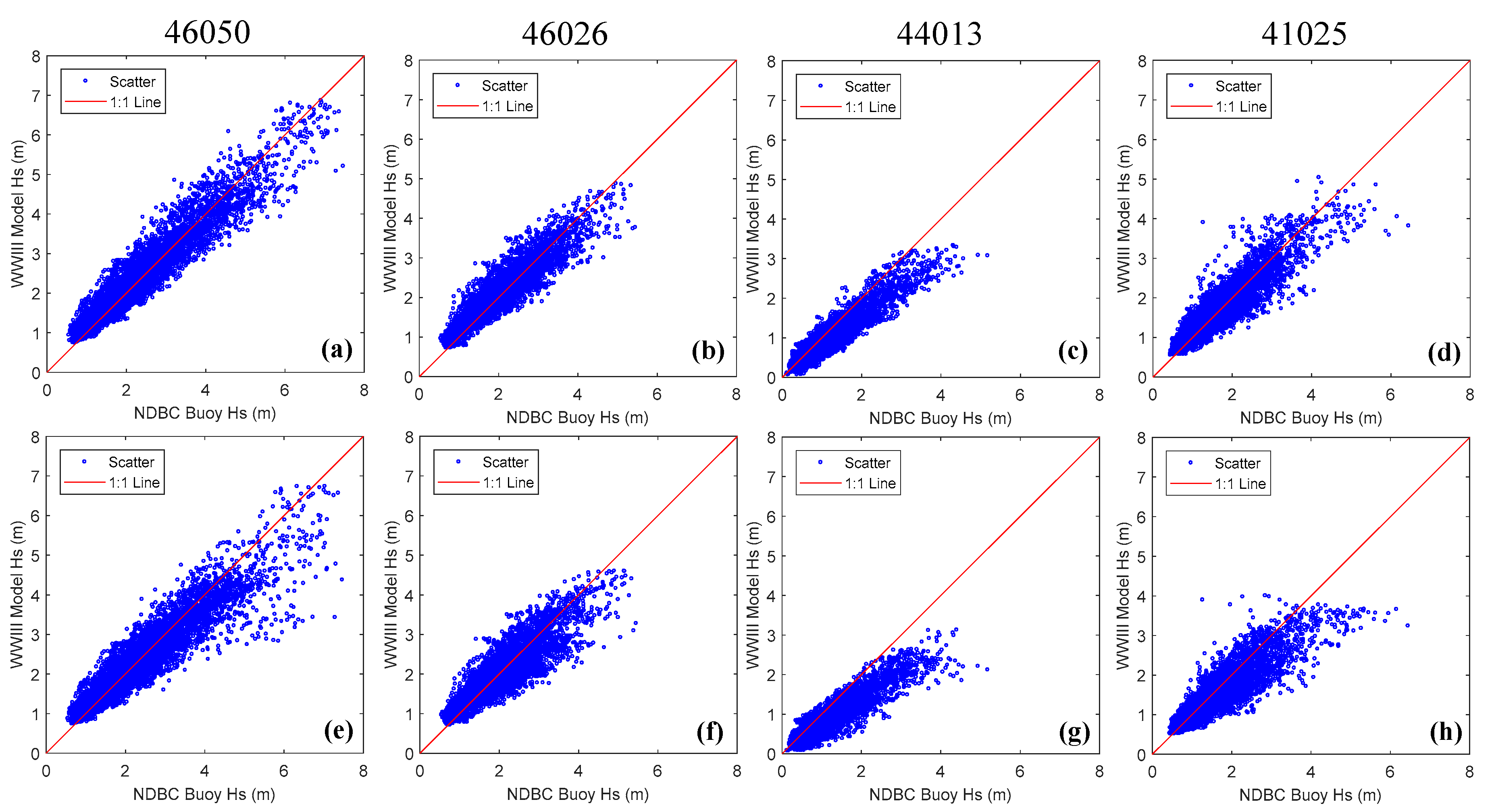
To investigate whether the regional wind product with higher spatial resolution can improve wave predictions, a sensitivity run using the NARR wind product was conducted for the nested WWIII model domains. In this test, the three-hourly NARR wind field was only applied to the WWIII 4′ domains due to its limited spatial coverage. The performance metrics for the yearly simulation results are summarized in Table 5. Compared to the baseline condition using the CFSR wind product, the NARR wind product appeared not to improve model predictions. In contrast, the results for those relatively large-wave events at all four buoys were even further under predicted, as indicated by the scatterplot comparisons (Figure 8). For instance, for an observed wave height > 5 m at 46050, >3 m at 46026, 44013, and 41025, the underprediction by the NARR wind becomes more apparent compared to that forced by the CFSR wind. This finding also agrees with that in the previous wind analysis that NARR wind shows a greater negative bias than the CFSR wind. This sensitivity test suggests regional wind-model products, such as NARR, do not produce better wave model results than those produced by the CFSR wind product, so they are not recommended for wave resource assessment modeling studies.
4. Conclusions
The sensitivity tests confirmed that wind forcing for the local domain is important in producing more accurate wave results and thus cannot be ignored. Although the observed wind forcing did not improve the models’ overall performance in predicting significant wave height, it did improve model predictions for large waves, which is crucial for the survival of WECs. This study also suggests that regional weather forecast products, such as NARR, do not necessarily improve wave model performance despite their finer spatial resolutions. On another note, only significant wave height was selected as a representative wave parameter to evaluate the wind forcing effect on large wave prediction. Although wave height is critical to assess the force and potential damage of large waves on WECs, other parameters, such as the wave period, should be considered to calculate the hydrodynamic force on WECs during extreme weather conditions (e.g., storms) [20,21]. Therefore, future work should include more systematic comparison of additional wave parameters.
Overall, the CFSR wind product is still considered one of the best global wind products for driving wind-wave simulations, as suggested by the 32-year wave hindcasts by NOAA using the CFSR wind [5]. The positive bias values for significant wave height at most stations except Buoy 44013, which is located on the U.S. East Coast, are also consistent with NOAA’s findings, which indicated that the positive bias was primarily caused by the inadequate swell dissipation algorithms in WWIII [5]. Because swells are most prominent in the Pacific Ocean, inadequate swell dissipation caused positive bias at the buoys on the U.S. West Coast. Interestingly, the positive bias was further amplified by UnSWAN at all buoys. The exact mechanism by which this amplification occurs warrants further investigation in future studies.
The improvement of large-wave predictions using observed wind suggests that the wind-sea model component is sensitive to wind forcing at local domains. However, the performance for the whole year did not show the same improvement. More research could be conducted on the spectral partition to identify the response of individual spectral components (e.g., swells, wind-sea) to various local wind-forcing products. Lastly, this study applied observed wind at a single buoy location for the entire local domain, which may underestimate the spatial variability of wind forcing across the domain. Better spatial interpolation methods would improve upon the accuracy of these results and should be considered in future studies.
Author Contributions
Conceptualization, Z.Y. and T.W.; Methodology, Z.Y. and T.W.; Validation, T.W. and W.-C.W.; Formal Analysis, Z.Y., T.W. and W.-C.W.; Investigation, Z.Y. and T.W.; Resources, Z.Y.; Data Curation, W.-C.W. and T.W.; Writing-Original Draft Preparation, T.W., Z.Y. and M.G.; Writing-Review & Editing, T.W., Z.Y., W.-C.W. and M.G.; Visualization, T.W. and W.-C.W.; Supervision, Z.Y.; Project Administration, Z.Y.; Funding Acquisition, Z.Y.
Funding
This study was funded by the Water Power Technology Office of the U.S. Department of Energy’s Office of Energy Efficiency and Renewable Energy, under Contract DE-AC05-76RL01830 to the Pacific Northwest National Laboratory.
Acknowledgments
The authors would like to thank the technical steering committee, chaired by Bryson Robertson at the West Coast Wave Initiative of the University of Victoria, for their oversight and input to this model study. Gabriel Garcia Medina at Pacific Northwest National Laboratory helped with Figure 6 and is also acknowledged.
Conflicts of Interest
The authors declare no conflict of interest.
Appendix A
The performance metrics are defined as follows:
The root mean square error (RMSE), or root mean square deviation, is defined as:
where is the number of observations, is the measured value, and is the predicted value.
The RMSE represents the sample standard deviation of the differences between predicted values and measured values.
The percentage error (PE) is defined as:
and is the average PE over the period of comparison.
The scatter index (SI) is the RMSE normalized by the average of all measured values over the value of comparison, where:
and where the overbar indicates the mean of the measured values.
Model bias, which represents the average difference between the predicted and measured value, is defined as:
Percentage bias, which is defined as:
is also commonly used to normalize bias.
The linear correlation coefficient, , is defined as:
and is a measure of the strength of the linear relationship between the predicted and measured values. In this study, R was tested at the significance level of 0.05.
References
- International Electrotechnical Commission. Marine Energy—Tidal and Other Water Current Converters—Part. 101: Wave Energy Resource Assessment and Characterization; Report No. IEC TS 62600-101; International Electrotechnical Commission: Geneva, Switzerland, 2015. [Google Scholar]
- Bidlot, J.-R.; Holmes, D.J.; Wittmann, P.A.; Lalbeharry, R.; Chen, H.S. Intercomparison of the performance of operational ocean wave forecasting systems with buoy data. Weather Forecast. 2002, 17, 287–310. [Google Scholar] [CrossRef]
- Pan, S.-Q.; Fan, Y.-M.; Chen, J.-M.; Kao, C.-C. Optimization of multi-model ensemble forecasting of typhoon waves. Water Sci. Eng. 2016, 9, 52–57. [Google Scholar] [CrossRef]
- Ellenson, A.; Özkan-Haller, H.T. Predicting large ocean wave events characterized by bimodal energy spectra in the presence of a low-level southerly wind feature. Weather Forecast. 2018, 33, 479–499. [Google Scholar] [CrossRef]
- Chawla, A.; Spindler, D.M.; Tolman, H.L. Validation of a thirty year wave hindcast using the climate forecast system reanalysis winds. Ocean Model. 2013, 70, 189–206. [Google Scholar] [CrossRef]
- Yang, Z.; Neary, V.S.; Wang, T.; Gunawan, B.; Dallman, A.R.; Wu, W.-C. A wave model test bed study for wave energy resource characterization. Renew. Energy 2017, 114, 132–144. [Google Scholar] [CrossRef]
- Wu, W.C.; Yang, Z.; Wang, T. Wave Resource Characterization Using an Unstructured Grid Modeling Approach. Energies 2018, 11, 605. [Google Scholar] [CrossRef]
- Chawla, A.; Spindler, D.; Tolman, H. WAVEWATCH III Hindcasts with Re-Analysis Winds. Initial Report on Model Setup; NOAA/NWS/NCEP Technical Note 291; NOAA: Silver Spring, MD, USA, 2011; 100p.
- Tolman, H.; WAVEWATCH III Development Group. User Manual and System Documentation of WAVEWATCH III Version 4.18; NOAA/NWS/NCEP Technical Note 316; NOAA: College Park, MD, USA, 2014; 311p.
- Zijlema, M. Computation of wind-wave spectra in coastal waters with swan on unstructured grids. Coast. Eng. 2010, 57, 267–277. [Google Scholar] [CrossRef]
- Saha, S.; Moorthi, S.; Pan, H.-L.; Wu, X.; Wang, J.; Nadiga, S.; Tripp, P.; Kistler, R.; Woollen, J.; Behringer, D.; et al. The NCEP climate forecast system reanalysis. Bull. Am. Meteorol. Soc. 2010, 91, 1015–1058. [Google Scholar] [CrossRef]
- Cavaleri, L. Wave modeling missing the peaks. J. Phys. Oceanogr. 2009, 39, 2757–2778. [Google Scholar] [CrossRef]
- Lenee-Bluhm, P.; Paasch, R.; Özkan-Haller, H.T. Characterizing the wave energy resource of the US Pacific Northwest. Renew. Energy 2011, 36, 2106–2119. [Google Scholar] [CrossRef]
- Garcá-Medina, G.; Özkan-Haller, H.T.; Ruggiero, P.; Oskamp, J. An inner-shelf wave forecasting system for the US Pacific Northwest. Weather Forecast. 2013, 28, 681–703. [Google Scholar] [CrossRef]
- Garcá-Medina, G.; Özkan-Haller, H.T.; Ruggiero, P. Wave resource assessment in Oregon and southwest Washington, USA. Renew. Energy 2014, 64, 203–214. [Google Scholar] [CrossRef]
- Neary, V.; Yang, Z.; Wang, T.; Gunawan, B.; Dallman, A.R. Model Test Bed for Evaluating Wave Models and Best Practices for Resource Assessment and Characterization; Sandia National Lab. (SNL-NM): Albuquerque, NM, USA, 2016.
- Jacobson, P.; Hagerman, G.; Scott, G. Mapping and Assessment of the United States Ocean Wave Energy Resource; Electric Power Research Institute: Palo Alto, CA, USA, 2011. [Google Scholar]
- Kilcher, L.; Thresher, R. Marine Hydrokinetic Energy Site Identification and Ranking Methodology Part I: Wave Energy; National Renewable Energy Lab (NREL): Golden, CO, USA, 2016.
- Ardhuin, F.; Rogers, E.; Babanin, A.; Filipot, J.-F.; Magne, R.; Roland, A.; van der Westhuysen, A.; Queffeulou, P.; Lefevre, J.-M.; Aouf, L. Semiempirical dissipation source functions for ocean waves. Part I: Definition, calibration, and validation. J. Phys. Oceanogr. 2010, 40, 1917–1941. [Google Scholar] [CrossRef]
- Alberello, A.; Chabchoub, A.; Gramstad, O.; Toffoli, A. Non-Gaussian properties of second-order wave orbital velocity. Coast. Eng. 2016. [Google Scholar] [CrossRef]
- Alberello, A.; Chabchoub, A.; Monty, J.P.; Nelli, F.; Lee, J.H.; Elsnab, J.; Toffoli, A. An experimental comparison of velocities underneath focussed breaking waves. Ocean Eng. 2018, 155. [Google Scholar] [CrossRef]
Figure 1.
Scatterplot comparisons of CFSR wind speed and observed wind speed at NDBC Buoys 46002 (a) and 46026 (b) in the northeast Pacific Ocean.
Figure 1.
Scatterplot comparisons of CFSR wind speed and observed wind speed at NDBC Buoys 46002 (a) and 46026 (b) in the northeast Pacific Ocean.

Figure 2.
(a) Locations of the four selected NDBC buoys (triangles) and the corresponding UnSWAN local domain boundaries. The NOAA’s 10-arc minute and 4-arc minute WWIII domain coverages for the U.S. West Coast and Atlantic Coast are also indicated in the figure. (b) The four UnSWAN model grids with depth contours.

Figure 3.
Performance statistics of three representative parameters ((a)—R; (b)—bias; and (c)—RMSE for all six wind products evaluated in this study. The correlation coefficient, R, is calculated at the significance level of α = 0.05 throughout this study.
Figure 3.
Performance statistics of three representative parameters ((a)—R; (b)—bias; and (c)—RMSE for all six wind products evaluated in this study. The correlation coefficient, R, is calculated at the significance level of α = 0.05 throughout this study.

Figure 4.
Time series comparisons of significant wave height between model simulations and buoy observations at all four buoys ((a)—46050; (b)—46026; (c)—41025; and (d)—44013) for the baseline-condition simulations in 2009.
Figure 4.
Time series comparisons of significant wave height between model simulations and buoy observations at all four buoys ((a)—46050; (b)—46026; (c)—41025; and (d)—44013) for the baseline-condition simulations in 2009.

Figure 5.
Comparison of significant wave heights between the baseline condition, no-wind condition, and buoy observations for the month of June (a–d) and November (e–h) in 2009.
Figure 5.
Comparison of significant wave heights between the baseline condition, no-wind condition, and buoy observations for the month of June (a–d) and November (e–h) in 2009.

Figure 6.
(a) Probability distributions of significant wave heights and (b) bivariate distribution of occurrence defined by the significant wave height and peak period for the baseline condition, observed-wind condition, and buoy observations in 2009.
Figure 6.
(a) Probability distributions of significant wave heights and (b) bivariate distribution of occurrence defined by the significant wave height and peak period for the baseline condition, observed-wind condition, and buoy observations in 2009.

Figure 7.
Comparison of significant wave heights between the baseline condition, observed-wind condition, and buoy observations at all four buoys ((a)—46050; (b)—46026; (c)—44013; and (d)—41025) for the example large-wave events in 2009.
Figure 7.
Comparison of significant wave heights between the baseline condition, observed-wind condition, and buoy observations at all four buoys ((a)—46050; (b)—46026; (c)—44013; and (d)—41025) for the example large-wave events in 2009.
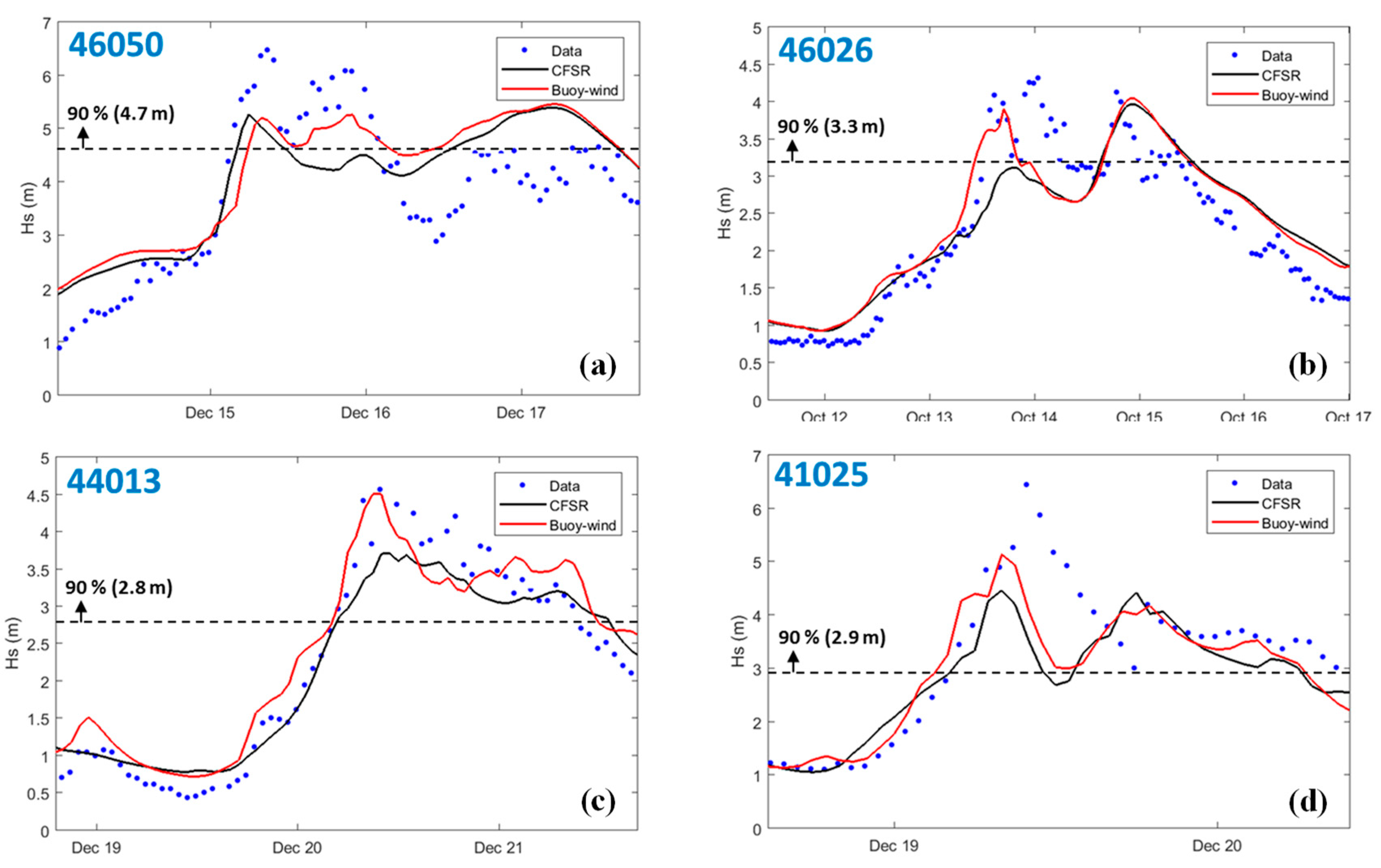
Figure 8.
Scatterplot of WWIII-predicted significant wave height vs. buoy observations for the baseline condition with the CFSR wind forcing (a–d) compared with those for the sensitivity run using the NARR wind forcing (e–h) at all four buoys.
Figure 8.
Scatterplot of WWIII-predicted significant wave height vs. buoy observations for the baseline condition with the CFSR wind forcing (a–d) compared with those for the sensitivity run using the NARR wind forcing (e–h) at all four buoys.


Table 1.
Evaluated wind-model products.
| Product Name | Spatial Coverage | Spatial Resolution | Temporal Range | Temporal Resolution | |
|---|---|---|---|---|---|
| CFSR | CFSR | Global | 0.5 degree | 1979–2010 | Hourly |
| CFSv2 | Global | 0.5 degree | 2011–present | Hourly | |
| ECMWF | ERA-Interim | Global | 0.703 degree | 1979–present | 3-hourly |
| ERA-20C | Global | 1.125 degree | 1900–2010 | 3-hourly | |
| GFS | Global | 0.5 degree | 2007–2014 | 3-hourly | |
| Global | 0.25 degree | 2015–present | 3-hourly | ||
| JRA | Global | 0.562 degree | 1957–2016 | 3-hourly | |
| NARR | North America | 32.463 km | 1979–present | 3-hourly | |
| NAM | North America | 12.19 km | 2004–present | 6-hourly | |
Table 2.
Designed model runs.
| Run# | Model Runs | Model Grids | Wind Forcing |
|---|---|---|---|
| 1 | Baseline WWIII | WWIII Domains | CFSR |
| 2 | Baseline UnSWAN | UnSWAN Domains | CFSR |
| 3 | UnSWAN without Wind | UnSWAN Domains | Zero |
| 4 | UnSWAN with Observed Wind | UnSWAN Domains | Observed |
| 5 | WWIII with NARR | WWIII Domains | CFSR + NARR |
Table 3.
Performance metrics for the WWIII and UnSWAN models.
| Model Run | Station | RMSE | PE (%) | SI | Bias | Bias (%) | R |
|---|---|---|---|---|---|---|---|
| WWIII | 46050 | 0.35 | 5.48 | 0.15 | 0.04 | 1.63 | 0.95 |
| 46026 | 0.30 | 8.57 | 0.16 | 0.09 | 4.63 | 0.93 | |
| 44013 | 0.30 | −13.55 | 0.31 | −0.17 | −17.21 | 0.94 | |
| 41025 | 0.31 | 7.34 | 0.20 | 0.05 | 2.95 | 0.91 | |
| UnSWAN | 46050 | 0.43 | 12.0 | 0.18 | 0.17 | 7.6 | 0.94 |
| 46026 | 0.33 | 12.0 | 0.16 | 0.15 | 8.2 | 0.93 | |
| 44013 | 0.24 | 7.0 | 0.25 | 0.0 | 0.1 | 0.93 | |
| 41025 | 0.35 | 10.0 | 0.22 | 0.08 | 5.3 | 0.87 |
Table 4.
Performance metrics for large (>90th percentile of significant wave height) waves only.
| Station | Wind | RMSE | PE (%) | SI | Bias | Bias (%) | R |
|---|---|---|---|---|---|---|---|
| 46050 | CFSR | 0.81 | −5.1 | 0.15 | −0.29 | −5.1 | 0.67 |
| Observed | 0.77 | −4.7 | 0.14 | −0.27 | −4.8 | 0.68 | |
| 46026 | CFSR | 0.49 | −5.2 | 0.13 | −0.22 | −5.6 | 0.57 |
| Observed | 0.48 | 2.4 | 0.12 | 0.08 | 2.0 | 0.58 | |
| 44013 | CFSR | 0.6 | −12.7 | 0.21 | −0.44 | −13.3 | 0.55 |
| Observed | 0.58 | −9.6 | 0.19 | −0.34 | −10.2 | 0.47 | |
| 41025 | CFSR | 0.83 | −9.9 | 0.25 | −0.41 | −11.0 | 0.47 |
| Observed | 0.69 | −5.2 | 0.2 | −0.23 | −6.4 | 0.55 |
Table 5.
Performance metrics for WWIII simulations with NARR wind.
| Station | Wind | RMSE | PE (%) | SI | Bias | Bias (%) | R |
|---|---|---|---|---|---|---|---|
| 46050 | CFSR | 0.35 | 5.48 | 0.15 | 0.04 | 1.63 | 0.95 |
| NARR | 0.43 | 1.50 | 0.19 | −0.06 | −2.87 | 0.93 | |
| 46026 | CFSR | 0.30 | 8.57 | 0.16 | 0.09 | 4.63 | 0.93 |
| NARR | 0.35 | 4.24 | 0.19 | 0.00 | 0.10 | 0.89 | |
| 44013 | CFSR | 0.30 | −13.55 | 0.31 | −0.17 | −17.21 | 0.94 |
| NARR | 0.40 | −21.75 | 0.41 | −0.26 | −26.08 | 0.92 | |
| 41025 | CFSR | 0.31 | 7.34 | 0.20 | 0.05 | 2.95 | 0.91 |
| NARR | 0.37 | −1.29 | 0.23 | −0.10 | −6.13 | 0.88 |
© 2018 by the authors. Licensee MDPI, Basel, Switzerland. This article is an open access article distributed under the terms and conditions of the Creative Commons Attribution (CC BY) license (http://creativecommons.org/licenses/by/4.0/).
Share and Cite
MDPI and ACS Style
Wang, T.; Yang, Z.; Wu, W.-C.; Grear, M. A Sensitivity Analysis of the Wind Forcing Effect on the Accuracy of Large-Wave Hindcasting. J. Mar. Sci. Eng. 2018, 6, 139. https://doi.org/10.3390/jmse6040139
AMA Style
Wang T, Yang Z, Wu W-C, Grear M. A Sensitivity Analysis of the Wind Forcing Effect on the Accuracy of Large-Wave Hindcasting. Journal of Marine Science and Engineering. 2018; 6(4):139. https://doi.org/10.3390/jmse6040139
Chicago/Turabian StyleWang, Taiping, Zhaoqing Yang, Wei-Cheng Wu, and Molly Grear. 2018. "A Sensitivity Analysis of the Wind Forcing Effect on the Accuracy of Large-Wave Hindcasting" Journal of Marine Science and Engineering 6, no. 4: 139. https://doi.org/10.3390/jmse6040139
Note that from the first issue of 2016, this journal uses article numbers instead of page numbers. See further details here.