Parametric Study of Tsunamis Generated by Earthquakes and Landslides


1
School of Engineering, University of Plymouth, Plymouth PL4 8AA, UK
2
Department of Civil and Environmental Engineering, The University of Auckland, Auckland 1142, New Zealand
3
Centre for Research in Earth Sciences, School of Geography, Earth and Environmental Sciences, University of Plymouth, Plymouth PL4 8AA, UK
*
Author to whom correspondence should be addressed.
J. Mar. Sci. Eng. 2019, 7(5), 154; https://doi.org/10.3390/jmse7050154
Submission received: 8 April 2019
/
Revised: 8 May 2019
/
Accepted: 10 May 2019
/
Published: 17 May 2019
(This article belongs to the Special Issue Tsunami Science and Engineering II)
Abstract
:Tsunami generation and propagation mechanisms need to be clearly understood in order to inform predictive models and improve coastal community preparedness. Physical experiments, supported by mathematical models, can potentially provide valuable input data for standard predictive models of tsunami generation and propagation. A unique experimental set-up has been developed to reproduce a coupled-source tsunami generation mechanism: a two-dimensional underwater fault rupture followed by a submarine landslide. The test rig was located in a 20 m flume in the COAST laboratory at the University of Plymouth. The aim of the experiments is to provide quality data for developing a parametrisation of the initial conditions for tsunami generation processes which are triggered by a dual-source. During the test programme, the water depth and the landslide density were varied. The position of the landslide model was tracked and the free surface elevation of the water body was measured. Hence the generated wave characteristics were determined. For a coupled-source scenario, the generated wave is crest led, followed by a trough of smaller amplitude decreasing steadily as it propagates along the flume. The crest amplitude was shown to be influenced by the fault rupture displacement scale, whereas the trough was influenced by the landslide’s relative density.
1. Introduction
Recently tsunamis have become the focus of renewed international research efforts after high profile events claimed thousands of lives in countries such as Indonesia, Japan, Thailand and Chile. It has been long known that coastal areas that are tectonically active are prone to tsunami inundations, as earthquakes generated by fault rupture are one of the most common tsunami triggering mechanisms. Usually, larger earthquake magnitudes (), cause more destructive tsunamis, which tend to be associated to thrust faulting [1]. However, strike-slip faults have also been associated with some of the most devastating events in history, e.g., the recent Palu earthquake and tsunami in September 2018. Furthermore, lower magnitude earthquakes are also capable of generating significant tsunamis and have been termed ‘tsunami earthquakes’ [2], e.g., Newfoundland earthquake () and tsunami in 1929, known as ‘The Grand Banks Tsunami’, which broke 12 submarine telegraph cables and is considered the Canada’s worst natural disaster [3]; and the Papua New Guinea earthquake () 1998, which generated a tsunami which struck the Northwest coast of Papua New Guinea with waves up to 10 m high and causing 15 m runup [4]. The aftermath of the Papua New Guinea tsunami was investigated by Tappin et al. [5], who found evidence of an offshore slump near Sissano Lagoon. Synolakis et al. [6] concurred with Tappin et al. [5] that a submarine landslide also contributed to the tsunami generation process, owing to the relatively moderate earthquake, the wave-height and run-up distributions, and wave arrival time [5]. Therefore, it is possible that coupled-source tsunamis, where submarine landslides are triggered by co-seismic shaking, might be more common than is realised. However, it is extremely difficult to get real time evidence/data of a submarine landslide owing to the unpredictably and accessibility of such events, although bathymetric surveys might help to locate areas prone to mass failure. High-resolution observational data are not generally feasible to obtain due to the complex location of occurrence for submarine landslides.
Consequently, the mechanics and kinematics of submarine landslides have yet to be studied in detail. Investigations of tsunamis generated by earthquakes are usually undertaken with numerical modelling of real data such as satellite, buoy and seismic records (e.g., [7,8,9,10]). Experimental modelling of underwater earthquakes is complex due to the difficulty of scaling the fault slip and geometry to water depth in a laboratory facility. Physical models of fault ruptures have been represented either by vertical motions of a plate or triangular moveable pistons, tested in two dimensional flume tanks [11,12,13]. The vast majority of previous investigations studying landslide generated tsunamis focused on subaerial landslides, both for physical [14,15,16,17], and numerical modelling [18,19], for which submarine landslide studies are also common [20,21,22]. There are also some experimental investigations of submarine landslide-induced tsunamis [23,24,25]. Usually, physical models of landslides consist of solid blocks of various geometries (e.g., triangular, semi-elliptic) [24,26,27] or a granular mass (i.e., [28,29]).
This investigation presents initial results from a novel coupled-source tsunami generation mechanism, which comprises a fault rupture and a fully-submarine landslide. Physical modelling of this dual mechanism will facilitate the investigation of complex interactions between the two tsunami sources and the affected water body.
2. Experimental Investigation
The test rig replicates two geological events: an underwater fault rupture followed by a submarine landslide. The fault rupture consists of a sudden uplift (up-thrust) of a plate, which is controlled by an electric actuator. A broad set of configurations were tested during each experimental campaign. Firstly, the fault rupture was tested in four different configurations: a horizontal plate uplift (HU), inclined slope uplift (IU), an inclined slope uplift with moving landslide (IU-ML) and an inclined slope uplift with fixed landslide (IU-FL). Moreover, different fault rupture uplift distances were performed: 0.06 m; 0.04 m; 0.02 m; 0.01 m and no displacement, in which case the landslide slid from the top of the slope under gravity (ML). Four water depths were used: 0.32 m; 0.27 m; 0.22 m and 0.165 m. Throughout the various experimental campaigns, different landslide models, as described in Section 2.3, were tested on the IU configuration. The measured parameters were: uplift displacement time-history, landslide position, and free surface elevation time-history.
2.1. Experimental Setup
The tsunami generation experiments were conducted in a 20 m long flume with a 0.6 × 0.6 m section (Figure 1). The test rig, which comprises a square plate (fault rupture model), bed slopes and landslide models, partially sits on a grill where water is normally recirculated when the flume is being used for current generation in its normal operation (Figure 2). The grill conveniently permits circulation of water when the uplift of the fault plate is performed preventing unwanted suction effects. The wave generation was restricted to one-way wave propagation by a backwall. A false floor was placed along the propagation area to provide sufficient clearance between the uplifted plate and the flume floor and to maintain a constant depth (Figure 2). The left most region of the test rig was obscured by the flume support (in blue, Figure 1), thus the camera field of view of the slope was restricted to an area of 0.175 m × 0.6 m within the glass walled region of the flume (Figure 2).
Resistance wave gauges (WG) were used to measure the surface elevation changes along the centreline of the flume. They consisted of a pair of 275 mm long 1.5 mm diameter stainless steel wires spaced 12.5 mm apart. In general, the gauges were approximately 0.3 m apart, but different gauge configurations between runs allowed to extend the surface elevation measurements further along the flume. Table 1 shows the wave gauge locations along the flume, where is the uplift back wall. Wave gauges in the near field were aligned at the changes in bathymetry and the initial location of the landslide (Figure 2). Note that WG1 location in this study corresponds to the location in [30], and WG2 to .
2.2. Fault Rupture Mechanism
Figure 3 shows the fault rupture model before it was located in the flume. The square plate, which represents the uplifted seafloor, is attached to two vertical side plates that slide up and down the flume walls on guide rails. The plate dimensions are 0.61 m side length (similar to Hammack [30]) by 0.6 m width (corresponding to the flume width). The vertical side plates are joined by a cross-brace where the actuator is attached to perform the uplifting motion. All plates are made of aluminium, the horizontal plate is 5 mm thick and the remaining elements are 10 mm thick to ensure they do not flex during the uplift motion. Stiffening bars were added to the plate to prevent it from bending due to the large uplift force. Two fault ruptures were replicated: a horizontal plate uplift and an inclined plate uplift. The addition of an inclined plane to the test rig enables the landslide to be released, which then slides down the slope, guided on PTFE runners. The benchmark configuration [31] of a 15 slope and a rigid semi-elliptical landslide model were adopted. The uplift motion performed by the actuator in the current investigation aims to reproduce the half-sine displacement time history of Hammack [30] with a maximum displacement of 60 mm, as later explained in Section 3.1.
2.3. Landslide Models
2.3.1. Solid Block Landslide
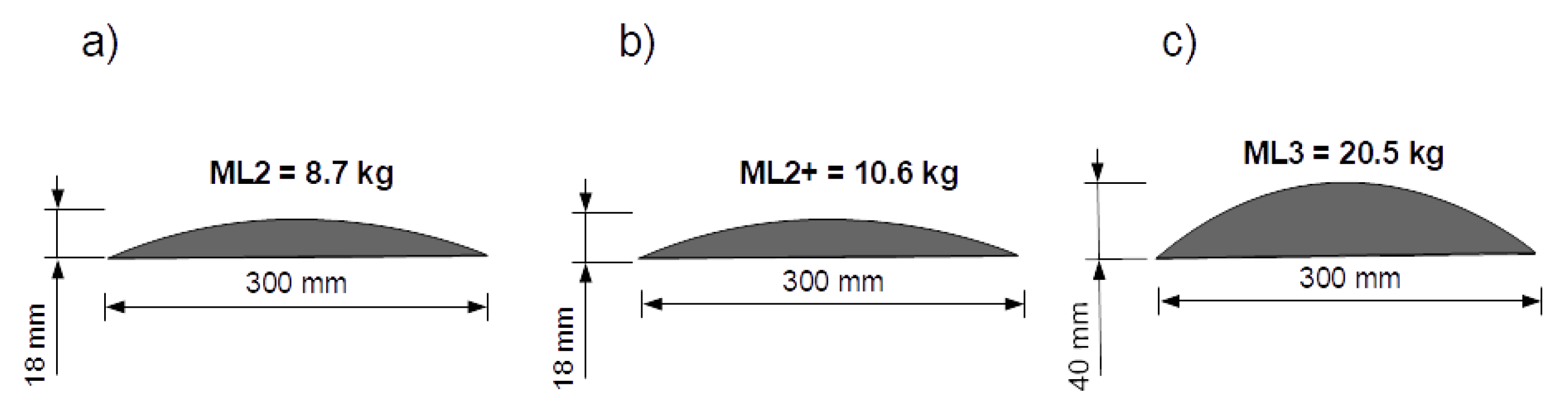
The landslide was represented by a semi-elliptical rigid body. Three landslide models with different thicknesses and densities were tested (Figure 4).
Models ML2 (8.7 kg) and ML2+ (10.6 kg) were hollow with a sealable bottom hatch to enable lead to be inserted to vary the mass of the model whilst keeping the volume constant. A bolt was fixed to the rear of the models as part of the release mechanism. The landslide was automatically released once the plate reached its maximum uplift displacement, at which point the bolt slid through a keyhole on the backwall. The landslide then moved downslope under gravity.
2.3.2. Modular Landslide
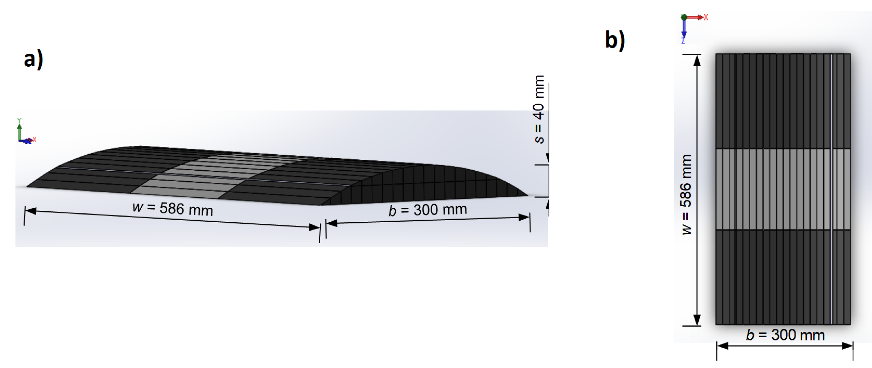
Model ML3 aimed to represent a granular landslide (Figure 5). The main feature of this model was its ability to change shape during its motion. This model consisted of twenty slices that were tested in differently grouped configurations, which were secured together with tape (Figure 5). To achieve the 20.5 kg weight, the landslide was constructed of a combination of stainless steel and aluminium. Two stainless steel rods were inserted through the uplift plate and the slope, and fixed onto the flume floor. When the uplift was performed, both plate and slope moved through the rods, leaving them flush once the required vertical distance was reached, releasing the landslide. This landslide had the advantage of being able to be tested in various configurations. In this paper, two sets of tests are presented for the modular landslide. The tests using the landslide as a whole solid block (all the slices attached together) are referred to as ML3, whilst the tests with independent sliding slices/blocks are referred to as ML3B.
3. Results
During the experimental programme, in addition to varying the water depth and the landslide size and density, four different fault rupture uplift distances were tested. Four non-dimensional parameters are used to report results: relative density , where is the landslide density, is the density of the water; landslide Froude number , where v is the landslide maximum velocity, g is the gravitational acceleration and h is the water depth; normalised wave height , where is the water surface elevation; and the displacement size scale , where is the vertical uplift displacement distance. The results were used to investigate the effects of both sources on the generated wave. Tests were first performed with each source separately before investigating the influence on the generated wave through a coupled-source tsunami event.
3.1. Description of Fault Rupture Motion
The plate uplift was tracked with a Photron Fastcam SAH 64Gb recording at 500 fps. Simultaneously, the actuator feedback was recorded. This feedback is the analog output from the encoder that reads the actuator motor response. Acquiring the video data allowed a comparison to the actuator’s feedback displacement data, providing confidence in the actuator values, which have been used in the subsequent analysis [32].
The uplift motion performed by the actuator in the current investigation aims to reproduce the half-sine displacement time history of Hammack [30] with a maximum displacement of 60 mm (Figure 6a). The theoretical displacement, is
where A is the maximum amplitude of the uplift and , where T is the sine wave period. Figure 6a shows a reasonable fit between the experimental data and the theoretical curve. The maximum amplitude and general shape of both curves are similar, but the measured data lags the theoretical curve.
The actuator uplift performance was not affected by the presence of the uplift plate or landslide models when performing the different test scenarios (Figure 6b): Horizontal Uplift (HU), Inclined Uplift (IU) and Inclined Uplift with Moving Landslide (IU-ML).
In contrast to Hammack [30], this study opted for an inclined uplift in order to incorporate a sliding landslide in later tests. Various incline-only (IU) combinations were tested and compared to Hammack’s results, as shown later in Section 3.3. To do so, Hammack’s non-dimensional parameters were adopted: amplitude scale , where is the maximum surface elevation measured at WG2, is the maximum uplift distance; displacement scale ; size scale , where where b is the fault rupture length; and the time-size ratio , where is the characteristic time of motion as defined by [30] for half-sine motion. Table 2 summarises those parameters.
Hammack [30] defined three characteristic motions according to the time-size ratio: impulsive (), transitional and creeping motion (). In the present study, the motions are predominantly transitional, with the exception of one (), where an uplift of 10 mm was performed in 370 mm water depth.
3.2. Description of Solid Block Motion
The landslide motion was tracked with a Nikon Digital Camera D5200 recording at 50 fps. Owing to the limited observational area (see Figure 2), the camera was placed at an oblique angle towards the landslide. Meticulous geometric camera calibration was required to obtain the camera intrinsic, extrinsic, and distortion coefficients, which were computed using the cameraCalibrator Matlab toolbox. These were later applied to the recorded video frames to correct the lens distortion and convert the camera pixels to real world units to obtain the correct dimensions of the tracked object. It was more feasible to apply image correction to this orientation compared with the uplift motion orientation, due to more manageable file sizes (i.e., 20.1 Mb for 8 s of video as opposed to the high-speed camera file which were around 34 Mb for 2 s of video).
The observed landslide motion for cases with no preceding uplift, is in good agreement with the following theoretical approximation (Figure 7a). A theoretical approximation for the landslide position was also obtained by considering a force balance (Appendix A), resulting in the following expression:
where x(t) is the landslide position along the slope at each instant in time t, m is the landslide mass, , b is the landslide length, w is the landslide width, is the drag coefficient, , is the slope angle, and is the landslide volume.
Grilli et al. [33] also developed a theoretical approximation for the motion of a submarine landslide sliding down an incline (Equation (3)). In this case, the landslide position at each instant of time was approximated using the observed acceleration and velocity values as follows
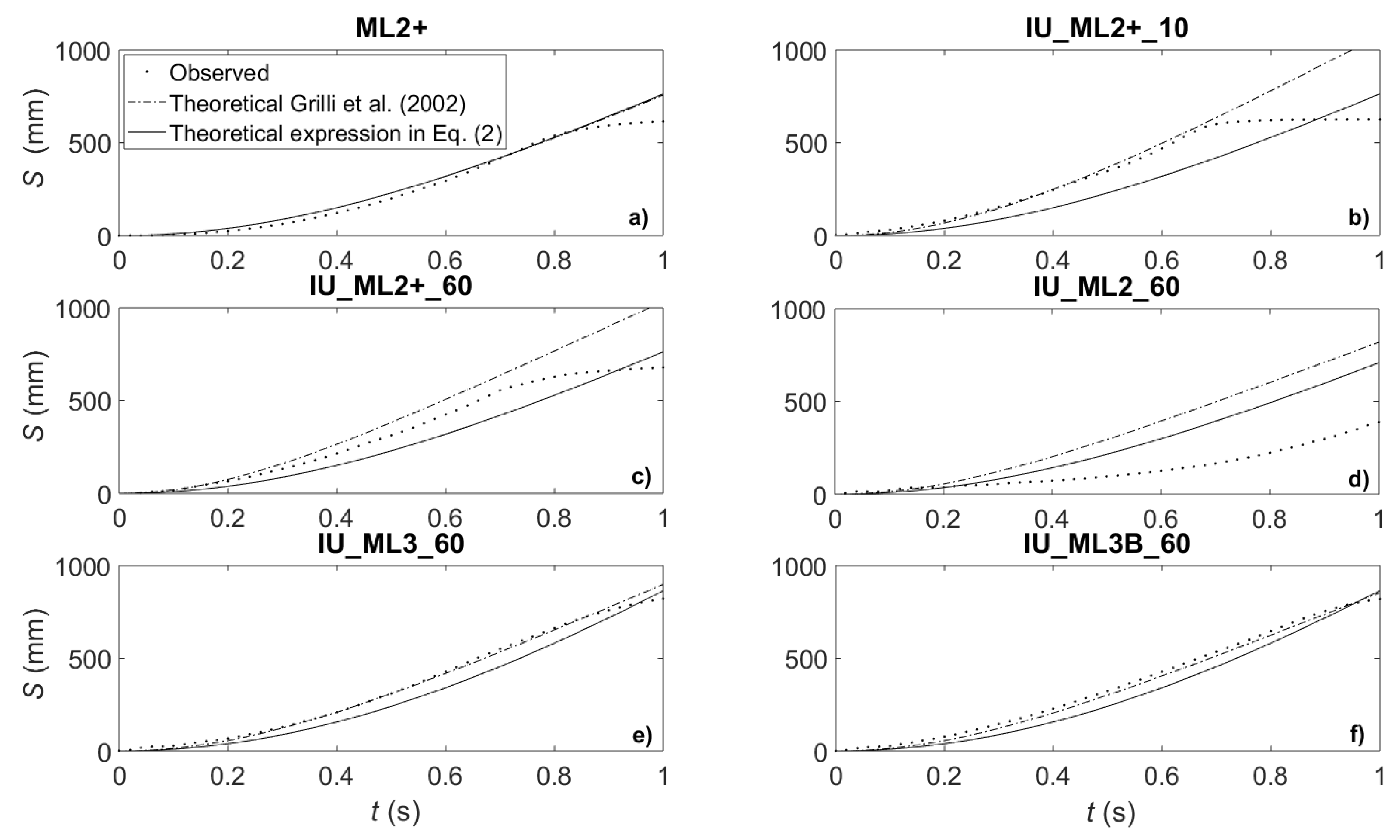
where is the landslide position along the slope at each instant in time t, and are the characteristic position and time of the landslide during its motion, as defined by [33]. Figure 7 shows a comparison of the observed data in this study, against the theoretical approximation from [33] and the theoretical approximation developed within this study. The parameters used for the theoretical approximations are summarised in Table 3.
Table 3 presents the landslide Froude number as a function of the relative density, where is the landslide Froude number, is the maximum velocity of the landslide, in relation to the relative density , where is the landslide density and = 1000 kg/m is the density of the water. For the landslide models ML2 and ML2+, increasing the relative density results in an increase in Froude number, and therefore increasing maximum velocity. ML3 has a greater relative density than ML2+, but a smaller Froude number, which means a slower maximum velocity. This smaller velocity of ML3 might be due to an increase in friction force, which depends on the landslide weight.
For all cases shown in Figure 7, the landslide motion was tracked from the same position on the slope, in 370 mm water depth. The following observations are made:
- Both theoretical approximations of landslide position show good agreement with the observed data for the landslide-only test (Figure 7a), until the point at which the landslide model experiences a change in geometry of the slope, not modelled by the theory.
- Whilst the ML2+ models (Figure 7a–c) stopped before transitioning onto the horizontal floor, the lighter model ML2 (Figure 7d) exhibited aquaplaning motion, travelling beyond the end of the slope. This resulted in longer travel times. The larger and heavier landslides ML3 and ML3B (Figure 7e,f), also exhibited longer travel times as they travelled beyond the end of the slope, due in part to their increased momentum and possibly due to deformation of the models (see final point).
- The effect of increasing uplift size on the ML2+ landslide position is also evident from these tests. The smallest uplift of 10 mm (Figure 7b), has measurements that are in very good agreement with the theoretical approximation of Grilli et al. [33], but rather poor agreement with the theoretical approximation from the present study. However, for a 60 mm uplift, observations from the same landslide model now have worse agreement with Grilli et al. [33], though match the present theory more closely than for the smaller uplift. It is worth noting that neither of the theoretical approximations took into account the uplift motion in their formulation.
- The landslide weight was seen to have a large effect on the level of agreement of the measured and theoretical predictions. For the same uplift magnitude of 60 mm, the lightest model ML2 (Figure 7c) exhibits the worst agreement, the medium mass model ML2+ (Figure 7b) exhibits slightly better agreement, and the largest model ML3 (Figure 7e) shows by far the best agreement. N.B. Model ML3 was thicker as well as heavier.
- As described in Section 2.3, ML3 consisted of twenty slices which were joined together with tape, which flexed as the landslide hit the end of the slope, enabling it to slightly adapt its shape as it moved onto the horizontal bed. For the case of the granular landslide ML3B (Figure 7f), the landslide is seen to travel slightly more slowly than ML3 (Figure 7e), possibly due to the spreading effect of the individual slices of ML3B during its motion, as opposed to ML3, which remained as a whole.
3.3. Effect of the Uplift Displacement on the Generated Wave
Figure 8 presents the surface elevation results for an inclined uplift-only test. The generated wave is crest-led with an amplitude slightly smaller than the performed uplift (nearly 30%) at WG1, decaying in amplitude as it propagates away from the test rig backwall (Figure 2). Soon after, the leading wave reaches WG3 on the transition from the incline into the horizontal false floor, there is a slight increase in the crest amplitude, which then decreases as it propagates further. Following the crest-led wave, there is a smaller elevation trough, which appears fairly constant for different uplift displacements (same water depth), as presented later in Figure 9. As opposed to the crest, the trough increases in amplitude as it propagates away from the backwall, though soon after it reached WG3, its amplitude starts decreasing. The dependence of the incline uplift displacements relative to the water depth () and the generated wave amplitude in the near-field is presented in Figure 9.
In general, for the same uplift displacement, an increase in water depth results in a decrease of crest and trough amplitude. The effect of the uplift is more pronounced on the crest amplitude than on the trough amplitude. The transfer of the uplift displacement to crest amplitude at WG2 is 70% for 20 mm uplift, 62% for 40 mm and 58% for 60 mm, in 300 mm water depth. This means that, for the same water depth, smaller uplift displacements generate a crest amplitude almost 10% larger than for larger displacements. For the case of a 60 mm uplift in 370 mm water depth, the surface elevation was measured at WG1, showing a displacement transfer of 70%, which is similar to the measured at WG2 for a 20 mm uplift. As presented in Hammack [11], Figure 10 shows the wave profiles for an inclined-only test.
As shown in Figure 10, the water rises to a maximum surface elevation, returning shortly after to a still water level. The maximum surface elevation reached depends upon the displacement size-ratio : smaller displacement size-ratios incurred larger amplitude scales (Figure 10). As mentioned in Section 3.1, the uplift displacements performed in this study are predominantly transitional, with one exception. This exception is the case of a 10 mm uplift in 370 mm water depth, which with a time-size ratio significantly below 1, classified by Hammack [30] as impulsive. This case also generated the largest amplitude scale, as shown in Figure 10h.
In the present study, the most similar size-scale to Hammack’s is . The variation of the relative amplitudes with the time size ratio for a range of uplift size ratios is compared to Hammack’s b/h = 1.22 in Figure 11. Similarly to Hammack’s half-sine motion, for the same time-size ratio and size-scale , the current study generated similar crest amplitudes, which also agree with Hammack’s Linear Theory [30]. For smaller size-scales , the present study generated smaller relative crest-amplitudes compared to Hammack [30], which might be due to the greater water depths tested in this study.
3.4. Effect of the Landslide Motion and Geometry on the Generated Wave
Figure 12 presents the surface elevation results for a landslide-only test. The generated wave is trough-led at WG1. As the trough propagates away from the back wall, its amplitude increases until it reaches WG4, close to where the landslide comes to rest, and the trough amplitude then starts decreasing. The trough is followed by a crest of smaller amplitude which propagates with a fairly constant amplitude until it reaches WG4, where its amplitude increased by almost half the initial crest amplitude. From WG6, a constant wave celerity of 1.6 m/s was observed, which was computed using the WG locations from Table 1. According the linear theory for shallow water waves (where the wavelength is much larger than the water depth), the phase velocity can be calculated as , where in this case m. With this, the theoretical phase velocity for the case presented in Figure 12 is 1.9 m/s. The difference between observed and theoretical wave celerity may be explained by dispersion effects, and/or friction induced by the flume walls.
As mentioned in Section 2.3, three different landslide models were tested. The effect of the landslide relative density on the amplitude of the generated wave in the near-field (WG1) is illustrated in Figure 13. Increasing relative densities result in increasing crest amplitude for all three landslide cases ML2, ML2+ and ML3 with a 60 mm uplift in 370 mm water depth, being more pronounced between ML2 and ML2+. For the case of the trough amplitude, it remains unchanged between ML2 and ML2+, which have the same dimensions but different masses. However, the ML3 trough amplitude increased (absolute value of what is presented in Figure 13) with respect to ML2+. This may be explained by the fact that the thickness of ML3 is about twice the thickness of ML2+ and its mass is also greater. Notice this trend is similar to the increase in crest amplitude between ML2+ and ML3.
For the case of the ‘modular’ landslide, two main configurations were tested: ML3 which is the landslide as a whole solid block, and ML3B which split into 20 slices when released. Figure 14 presents a comparison of the surface elevation changes for two tests with inclined uplift and landslide models ML3 and ML3B. The effect of the fragmentation of the landslide on the generated wave is only visible at WG1 (blue lines), where the crest amplitude is around 15 mm larger for ML3 than for ML3B. This reduction in amplitude might be due to the spreading of the landslide ML3B as it slides down the incline, meaning a reduced thickness of the landslide.
3.5. Effect of a Coupled Mechanism on the Generated Wave
Figure 15 presents surface elevation profiles obtained from the wave gauges at different instants of time. Axes on the left are true scale, representing the water depth in millimetres. Axes on the right represent the surface elevation changes, which have been exaggerated ten times for clarity. Two sets of data are presented: inclined uplift-only test in grey colour and inclined uplift followed by landslide ML3 in black, both with uplift distance of 60 mm and water depth of 370 mm. The first three plots in Figure 15 capture the uplift, which happens much faster than the landslide motion, hence the small time step between them. This uplift generates the wave and contributes mainly to a crest, as mentioned earlier and illustrated in Figure 8. As soon as the landslide starts its motion, the trough of the wave increases in amplitude (from s). Notice that the landslide front edge is always following the wave crest.
4. Discussion
This paper has presented a novel physical model of a coupled-mechanism for tsunami generation involving a fault rupture, which was designed based on the prominent study by Hammack [30], and a submarine landslide, which was designed following the benchmark recommendations by Watts et al. [31]. Results from the first iteration of experiments were reported, where the coupled-sources were co-located and the landslide was released instantaneously after the fault rupture had reached the maximum uplift distance. Each source motion and the resulting wave characteristics of the source motion and generated waves have been used to understand the wave generation properties.
The current study found that for the same uplift displacement, the influence of an increasing water depth on the generated wave was a decrease of the crest amplitude, as in Hammack [30] and Todorovska & Trifunac [9]. However, owing to the space underneath the uplifted plate of this study, the generated wave amplitude was not equal to the uplift displacement. This behaviour was observed in Hammack [30], where the uplift mechanism consisted of a sealed unit, with no water exchange between chambers. It is also worth noting that the transition between the inclined and the horizontal plane seemed to have an influence on the generated wave, as explained in Section 3.3 and illustrated in Figure 8, where the generated crest amplitude decreased as it propagated away from the back wall, until it reached WG4 (transition from slope to horizontal flume floor at WG3), where an increase in amplitude was observed, to then decrease again. A similar behaviour was observed for the trough amplitude, in which the amplitude fluctuation happened at WG3.
Regarding the case of the submarine landslide only tests (without uplift), the generated wave in the near-field (WG1 and WG2) was trough led, which was also found by others such as [24,31]. In general, increasing the relative landslide density and thickness meant an increase in the crest amplitude and a slight decrease in the trough amplitude. The thickness of the landslide model was seen to have an effect on the trough amplitude of the generated wave. For the case of ML3, whose thickness was twice that of ML2, the increase in relative density meant an increase in the trough amplitude. For the case of the granular landslide, only the crest amplitude was affected by the fragmentation of the block, being around 15 mm smaller than the equivalent crest amplitude generated by ML3. As suggested in Section 3.4, the reason might have been that landslide ML2 was observed to aquaplane at the end of its motion down the incline, when it transitioned onto the horizontal plane (false floor).
The most obvious finding to emerge from the coupled-mechanism analysis is that the crest amplitude is mainly controlled by the uplift displacement, whereas the trough amplitude is influenced by the landslide motion.
Limitations and Future Work
The present study encountered various limitations, mainly due to the restricted capabilities of the test rig. The main limitation for the fault rupture model was the distance underneath the uplifted plate, under which water was recirculated. This issue was reflected in the resulting crest amplitude, particularly in inclined uplift only tests (IU), which is around 70% of the largest uplift displacement performed in the present study. In contrast, Hammack [30] performed the uplift by pushing the plate from underneath the flume floor, transferring the complete uplift distance onto the generated wave amplitude, since no volume of water was transferred elsewhere except to the generated wave. For the case of the landslide, owing to hardware limitations such as the difficulty of cable routing an accelerometer around the complex test rig, it could only be tracked using a digital camera, as opposed to placing an accelerometer inside it as in previous experimental studies dealing with submarine landslides [24,34]. There is no motion data for landslide only tests for model ML3, owing to the difficulty of releasing this model without performing the uplift, since it was extremely heavy for the retention mechanism.
Future research should be undertaken to overcome the experimental constraints. Firstly, it is to minimise or eliminate the gap underneath the fault rupture model so that the uplifted volume of water is fully transferred into the generated wave. Secondly, to overcome landslide motion tracking issues, either by having a clear observation window from which its motion can be fully tracked, or by installing a waterproof accelerometer inside the models. With these improvements, a more robust dataset could be developed and a better understanding of the generated wave properties could be obtained. Moreover, the coupled-source set up could be implemented to introduce a delay between the earthquake and the landslide, which would be closer to real cases. Furthermore, comparisons with numerical models such as SPH (Smooth Particle Hydrodynamics) would be facilitated if more robust data is provided to validate the models. A first SPH study investigating the fault rupture triggering mechanism for tsunami generation was developed by [35], showing good agreement for preliminary tests performed with an horizontal uplift only. Further simulations will investigate the inclined uplift and the inclusion of the submarine landslide.
5. Conclusions
The present study was carried out to develop a two dimensional novel coupled-source tsunami generator and to determine the generated wave properties in relation to the sources parameters. Experiments were undertaken to investigate the main feature of each source separately, which were in agreement with previous studies. These experiments confirmed that there is a noticeable influence from the secondary source (landslide) in the generation process. The key finding is that the generated wave is crest led, followed by a trough of smaller amplitude and decreasing steadily as it propagates along the flume. The crest amplitude was shown to be controlled by the fault rupture displacement scale, for which smaller displacement scales produced larger amplitude scales, whereas the trough was controlled by the landslide’s relative density, where larger relative amplitudes produced larger relative trough amplitudes.
This paper has developed a novel tsunami mechanism which provided a deeper insight into the source parameters influencing a coupled-source tsunami generation scenario. These results add to the rapidly expanding field of submarine landslides as tsunami triggers, specially when combined with a co-seismic event. The major limitation of this study is the impossibility of achieving a scalable model to generate a tsunami-like wave, owing to the facility restrictions, e.g., flume tank dimensions, limited water depth, actuator placement. It was not possible to test the granular landslide without performing an uplift; therefore, it is unknown if the lack of an uplift would have influenced the landslide’s motion, which could have a major effect on the generated wave. The limitations of scaling landslide-generated wave in a laboratory facility were examined by Heller et al. [36]. The scale effects were found to reduce the relative wave amplitude following the actuator placement.
Further experimental work will involve studying other spatial/dynamic features of various uplift motions, e.g., exponential, impulsive, as well as more complex landslide models, e.g., highly dispersive granular landslides. Beyond tsunami-oriented experiments, the current results will be used to develop numerical models which could facilitate the investigation of more realistic tsunami scenarios (e.g., to scale).
Author Contributions
Conceptualization, C.W.; methodology, N.P.d.P.P.; data analysis, N.P.d.P.P.; investigation, N.P.d.P.P.; writing—original draft preparation and editing, N.P.d.P.P.; writing—review, N.P.d.P.P., A.R., C.W., S.J.B.; supervision, A.R., C.W., S.J.B.; project administration, A.R.; funding acquisition, A.R.
Funding
This research was undertaken with the support of a PhD studentship jointly funded by the Marine Institute and the Sustainable Earth Institute of the University of Plymouth.
Acknowledgments
We are grateful for the technical support of the COAST Laboratory (University of Plymouth) technicians, who provided insight and expertise that greatly assisted the experiments.
Conflicts of Interest
The authors declare no conflict of interest.
Appendix A. Theoretical Formulation for Landslide Motion
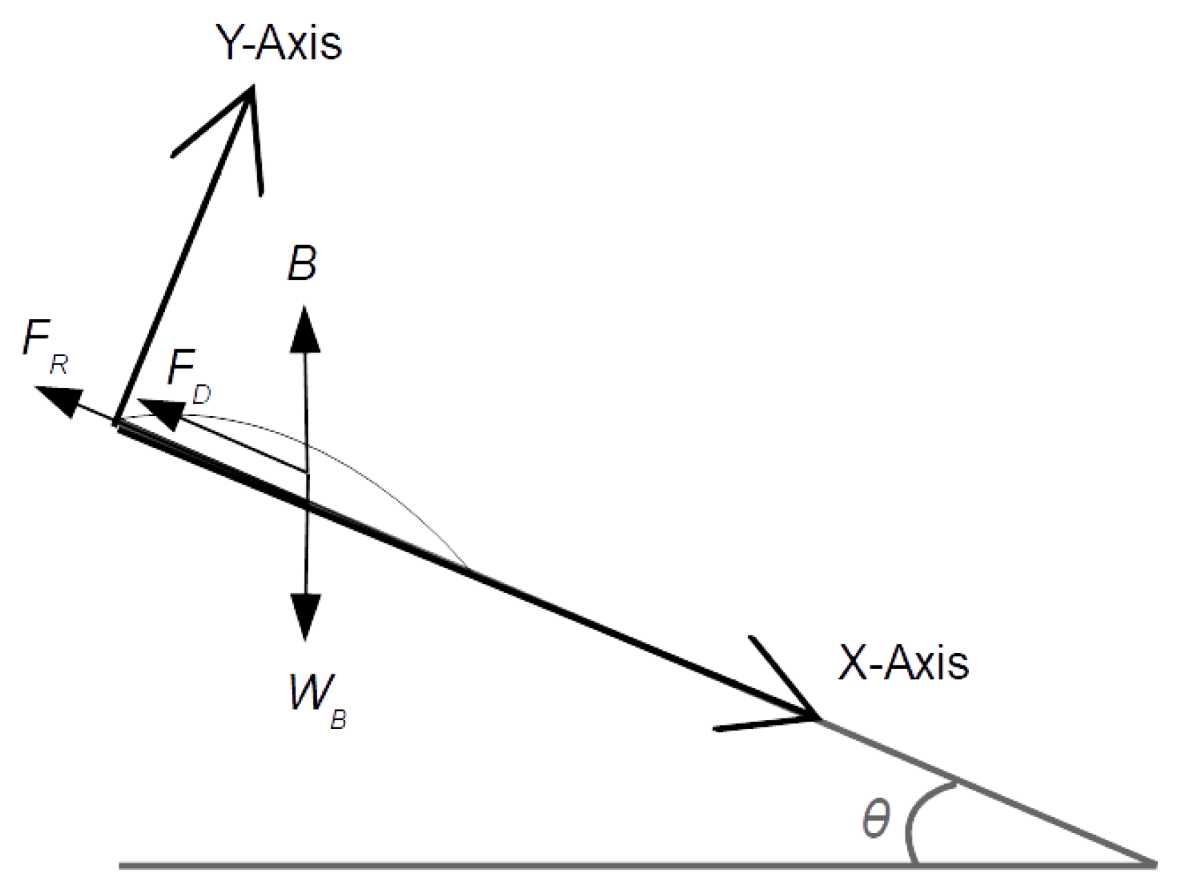
Figure A1 shows a free body diagram for the sliding motion of the landslide down the incline. Considering Newton’s second law , where m is the landslide mass and a is the landslide acceleration, and the X-axis on the slope (Figure A1), then the acceleration of the landslide can be expressed as .
Figure A1.
Free body diagram for landslide motion.

The force balance is
where W is the landslide weight, B is the buoyancy force, is the drag force, is the frictional force, is the slope angle. Re-arranging Equation (A1) gives:
The drag force depends on the landslide velocity v to the second power , where is the density of water, b is the landslide length and w is the landslide width. To facilitate further operations, the term representing the drag force is simplified to , where D represents the coefficients multiplying the velocity in the drag force expression, and . The terms on the right hand side of Equation (A2) are constant and can be grouped as . Grilli et al. [33] neglected the friction force to obtain his equation of motion for the submarine landslide. In the present study, as the materials employed to construct the slope have a very low friction coefficient (PTFE), the friction force is also neglected. Therefore, the term , and the re-arranged second order differential equation is of the form:
Using the substitution then gives:
Note that the apostrophe indicates derivative. This is . Equation (A4) may be rewritten as
By integrating Equation (A6), if , a particular solution can be obtained. The solution to Equation (A6) is:
For , , and therefore the . Now z is isolated as follows:
With the logarithm property , , Equation (A8) may be rewritten as:
Re-arranging the expression in Equation (A9) we obtain:
Note than , and therefore Equation (A10) may be re-arranged as:
Note that Equation (A11) represents the landslide velocity at each instant in time. The integration of Equation (A11) gives the landslide position at each instant of time:
Note that . Furthermore, , therefore and , which makes .
References
- Okal, E.A. Seismic parameters controlling far-field tsunami amplitudes: A review. Nat. Hazards 1988, 1, 67–96. [Google Scholar] [CrossRef]
- Kajiura, K. Tsunami source, energy and directivity of wave radiation. Bull. Earthq. Res. Inst. 1970, 48, 835–869. [Google Scholar]
- Fine, I.V.; Rabinovich, A.B.; Bornhold, B.D.; Thomson, R.E.; Kulikov, E.A. The Grand Banks landslide-generated tsunami of November 18, 1929: Preliminary analysis and numerical modeling. Mar. Geol. 2005, 215, 45–57. [Google Scholar] [CrossRef]
- Kawata, Y.; Benson, B.C.; Borrero, J.C.; Borrero, J.L.; Davies, H.L.; Lange, W.P.; Imamura, F.; Letz, H.; Nott, J.; Synolakis, C.E. Tsunami in Papua New Guinea was as intense as first thought. Eos Trans. Am. Geophys. Union 1999, 80, 101–105. [Google Scholar] [CrossRef]
- Tappin, D.R.; Watts, P.; McMurtry, G.M.; Matsumoto, T. Offshore evidence on the source of the 1998 Papua New Guinea tsunami: A sediment slump. In Proceedings of the International Tsunami Symposium, Seattle, WA, USA, 7–10 August 2001; Volume 175, pp. 381–388. [Google Scholar]
- Synolakis, C.E.; Bardet, J.P.; Borrero, J.C.; Davies, H.L.; Okal, E.A.; Silver, E.A.; Sweet, S.; Tappin, D.R. The slump origin of the 1998 Papua New Guinea Tsunami. Proc. R. Soc. Math. Phys. Eng. Sci. 2002, 458, 763–789. [Google Scholar] [CrossRef]
- Heinrich, P.; Guibourg, S.; Roche, R. Numerical modeling of the 1960 Chilean tsunami. Impact on French Polynesia. Phys. Chem. Earth 1996, 21, 19–25. [Google Scholar] [CrossRef]
- Stein, R.S. The role of stress transfer in earthquake occurrence. Nature 1999, 402, 605–609. [Google Scholar] [CrossRef]
- Todorovska, M.I.; Trifunac, M.D. Generation of tsunamis by a slowly spreading uplift of the sea floor. Soil Dyn. Earthq. Eng. 2001, 21, 151–167. [Google Scholar] [CrossRef]
- Kowalik, Z.; Knight, W.; Logan, T.; Whitmore, P. The tsunami of 26 December, 2004: Numerical modeling and energy considerations. Pure Appl. Geophys. 2007, 164, 379–393. [Google Scholar] [CrossRef]
- Hammack, J.L. A note on tsunamis: Their generation and propagation in an ocean of uniform depth. J. Fluid Mech. 1973, 60, 769–799. [Google Scholar] [CrossRef]
- Iwasaki, S. Experimental study of a tsunami generated by a horizontal motion of a sloping bottom. Bull. Earthq. Res. Inst. 1982, 57, 239–262. [Google Scholar]
- Jamin, T.; Gordillo, L.; Ruiz-Chavarria, G.; Berhanu, M.; Falcon, E. Experiments on generation of surface waves by an underwater moving bottom. Proc. R. Soc. Math. Phys. Eng. Sci. 2015, 471. [Google Scholar] [CrossRef]
- Heller, V.; Hager, W.H. Impulse product parameter in landslide generated impulse waves. J. Waterw. Port Coast. Ocean. Eng. 2010, 136, 145–155. [Google Scholar] [CrossRef]
- Heller, V.; Spinneken, J. Improved landslide-tsunami prediction: Effects of block model parameters and slide model. J. Geophys. Res. Ocean. 2013, 118, 1489–1507. [Google Scholar] [CrossRef]
- Heller, V.; Bruggemann, M.; Spinneken, J.; Rogers, B.D. Composite modelling of subaerial landslide–tsunamis in different water body geometries and novel insight into slide and wave kinematics. Coast. Eng. 2016, 109, 20–41. [Google Scholar] [CrossRef]
- Evers, F.M.; Hager, W. Generation and spatial propagation of landslide generated impulse waves. Coast. Eng. Proc. 2017, 1, 13. [Google Scholar] [CrossRef]
- Assier-Rzadkieaicz, S.; Heinrich, P.; Sabatier, P.C.; Savoye, B.; Bourillet, J.F. Numerical modelling of a landslide-generated tsunami: The 1979 Nice event. Pure Appl. Geophys. 2000, 157, 1707–1727. [Google Scholar] [CrossRef]
- Tinti, S.; Pagnoni, G.; Zaniboni, F. The landslides and tsunamis of the 30th of December 2002 in Stromboli analysed through numerical simulations. Bull. Volcanol. 2006, 68, 462–479. [Google Scholar] [CrossRef]
- Heinrich, P.; Piatanesi, A.; Hébert, H. Numerical modelling of tsunami generation and propagation from submarine slumps: The 1998 Papua New Guinea event. Geophys. J. Int. 2001, 145, 97–111. [Google Scholar] [CrossRef]
- Lynett, P.; Liu, P.L.F. A numerical study of submarine-landslide-generated waves and run-up. Proc. R. Soc. Math. Phys. Eng. Sci. 2002, 458, 2885–2910. [Google Scholar] [CrossRef]
- Bondevik, S.; Løvholt, F.; Harbitz, C.; Mangerud, J.; Dawson, A.; Svendsen, J.I. The Storegga Slide tsunami—Comparing field observations with numerical simulations. In Ormen Lange—An Integrated Study for Safe Field Development in the Storegga Submarine Area; Elsevier: New York, NY, USA, 2005; pp. 195–208. [Google Scholar]
- Watts, P. Tsunami features of solid block underwater landslides. J. Waterw. Port Coast. Ocean. Eng. 2000, 2, 144–152. [Google Scholar] [CrossRef]
- Sue, L.P. Modelling of Tsunami Generated by Submarine Landslides. Ph.D. Thesis, University of Canterbury, Christchurch, New Zealand, 2007. [Google Scholar]
- Van Nieuwkoop, J.C.C. Experimental and Numerical Modelling of Tsunami Waves Generated by Landslides. Master’s Thesis, Delft University of Technology, Delft, The Netherlands, 2007. [Google Scholar]
- Wiegel, R.L. Laboratory studies of gravity waves generated by the movement of a submerged body. Eos Trans. Am. Geophys. Union 1955, 36, 759–774. [Google Scholar] [CrossRef]
- Watts, P.; Grilli, S.T. Underwater landslide shape, motion, deformation, and tsunami generation. Int. Offshore Polar Eng. Conf. 2003, 5, 364–371. [Google Scholar]
- Heller, V.; Hager, W.H. Wave types of landslide generated impulse waves. Ocean. Eng. 2011, 38, 630–640. [Google Scholar] [CrossRef]
- Mohammed, F.; Fritz, H.M. Physical modeling of tsunamis generated by three-dimensional deformable granular landslides. J. Geophys. Res. Ocean. 2012, 118, 3221. [Google Scholar] [CrossRef]
- Hammack, J.L. Tsunamis—A Model of Their Generation and Propagation. Ph.D. Thesis, California Institute of Technology, Pasadena, CA, USA, 1972. [Google Scholar]
- Philip, W.; Fumihiko, I.; Aaron, B.; Grilli, S.T. Benchmark cases for tsunamis generated by underwater landslides. In Proceedings of the Fourth International Symposium on Ocean Wave Measurement and Analysis, San Francisco, CA, USA, 2–6 September 2001. [Google Scholar] [CrossRef]
- Perez del Postigo, N.; Raby, A.; Whittaker, C.; Boulton, S.J. Tsunami generation by combined fault rupture and landsliding. In Proceedings of the 7th International Conference on the Application of Physical Modelling in Coastal and Port Engineering and Science (Coastlab18), Santander, Spain, 22–26 May 2018; pp. 1–10. [Google Scholar]
- Grilli, S.T.; Vogelmann, S.; Watts, P. Development of a 3D numerical wave tank for modeling tsunami generation by underwater landslides. Eng. Anal. Bound. Elem. 2002, 26, 301–313. [Google Scholar] [CrossRef]
- Whittaker, C.; Nokes, R.; Davidson, M. Tsunami forcing by a low Froude number landslide. Environ. Fluid Mech. 2015, 15, 1215–1239. [Google Scholar] [CrossRef]
- Wana, R.; Perez, N.; Hughes, J.; Graham, D.; Raby, A.; Whittaker, C. Smoothed Particle Hydrodynamics (SPH) modelling of tsunami waves generated by a fault rupture. In Proceedings of the ASME 2007 26th International Conference on Offshore Mechanics and Arctic Engineering, San Diego, CA, USA, 10–15 June 2019. [Google Scholar]
- Heller, V.; Hager, W.H.; Minor, H.E. Scale effects in subaerial landslide generated impulse waves. Exp. Fluids 2008, 44, 691–703. [Google Scholar] [CrossRef]
Figure 1.
Sketch of the 20 m two dimensional flume of the Coast Laboratory (University of Plymouth). The yellow dashed lines mark the area where the test rig was placed. (a) Plan view. (b) Cross-section.
Figure 1.
Sketch of the 20 m two dimensional flume of the Coast Laboratory (University of Plymouth). The yellow dashed lines mark the area where the test rig was placed. (a) Plan view. (b) Cross-section.

Figure 2.
Schematic diagram (not to scale) of the test rig showing the fault rupture (uplift plate) and landslide model. WG indicates resistance wave gauges used to measure the surface elevation changes. The dashed red lines show the camera field of view.
Figure 2.
Schematic diagram (not to scale) of the test rig showing the fault rupture (uplift plate) and landslide model. WG indicates resistance wave gauges used to measure the surface elevation changes. The dashed red lines show the camera field of view.

Figure 3.
Photograph showing the fault rupture model.

Figure 4.
Cross-sections sketch of landslide models: (a) ML2, (b) ML2+, and (c) ML3 and ML3B (same dimensions, divided in slices (Figure 5)).
Figure 4.
Cross-sections sketch of landslide models: (a) ML2, (b) ML2+, and (c) ML3 and ML3B (same dimensions, divided in slices (Figure 5)).

Figure 5.
(a) ML3 landslide model geometry and dimensions. (b) Top view of ML3. Light grey slices are made of solid stainless steel machined bars. Black slices are made of aluminium machined bars.
Figure 5.
(a) ML3 landslide model geometry and dimensions. (b) Top view of ML3. Light grey slices are made of solid stainless steel machined bars. Black slices are made of aluminium machined bars.

Figure 6.
(a) Plate displacement () time history, comparing experimental data with a fitted half-sine curve as in Hammack [30]. (b) Plate displacement () time history for the different test scenarios: Horizontal Uplift (HU), Inclined Uplift (IU) and Inclined Uplift with Moving Landslide (IU-ML).
Figure 6.
(a) Plate displacement () time history, comparing experimental data with a fitted half-sine curve as in Hammack [30]. (b) Plate displacement () time history for the different test scenarios: Horizontal Uplift (HU), Inclined Uplift (IU) and Inclined Uplift with Moving Landslide (IU-ML).

Figure 7.
Observed data compared to theoretical approximations for landslide models (a) without and, (b) with an uplift of 10 mm, and (c–f) with an uplift of 60 mm in 370 mm water depth.
Figure 7.
Observed data compared to theoretical approximations for landslide models (a) without and, (b) with an uplift of 10 mm, and (c–f) with an uplift of 60 mm in 370 mm water depth.

Figure 8.
Surface elevation time histories for an inclined uplift test of 60 mm in 370 mm water depth.
Figure 8.
Surface elevation time histories for an inclined uplift test of 60 mm in 370 mm water depth.

Figure 9.
Relative crest and trough amplitudes () at WG2 as a function of displacement scales for IU only. Note that the squares represent the relative wave height.
Figure 9.
Relative crest and trough amplitudes () at WG2 as a function of displacement scales for IU only. Note that the squares represent the relative wave height.

Figure 10.
Dimensionless surface elevations as a function of dimensionless time at WG1 (blue) and WG2 (red) for an inclined uplift-only (IU).
Figure 10.
Dimensionless surface elevations as a function of dimensionless time at WG1 (blue) and WG2 (red) for an inclined uplift-only (IU).

Figure 11.
Variation of relative wave amplitude with the time size ratio at WG2 () for a half-sine motion (IU only).
Figure 11.
Variation of relative wave amplitude with the time size ratio at WG2 () for a half-sine motion (IU only).

Figure 12.
Surface elevation time histories for an landslide only test in 370 mm water depth. The dashed line represents the constant wave celerity.
Figure 12.
Surface elevation time histories for an landslide only test in 370 mm water depth. The dashed line represents the constant wave celerity.

Figure 13.
Normalised wave height measured at WG1 for different landslide relative density for cases with an uplift of 60 mm and 370 mm water depth.
Figure 13.
Normalised wave height measured at WG1 for different landslide relative density for cases with an uplift of 60 mm and 370 mm water depth.

Figure 14.
Surface elevation time histories for an inclined uplift of 60 mm and landslide model ML3 (solid lines), or ML3B (dashed lines) in 370 mm water depth.
Figure 14.
Surface elevation time histories for an inclined uplift of 60 mm and landslide model ML3 (solid lines), or ML3B (dashed lines) in 370 mm water depth.

Figure 15.
Stacked plots showing the setup with the surface elevation time histories for uplift-only tests (grey) and uplift followed by landslide ML3 for a 60 mm uplift and 370 mm water depth. The displacement time histories for the fault rupture are shown as the plate lifts up between s and s.
Figure 15.
Stacked plots showing the setup with the surface elevation time histories for uplift-only tests (grey) and uplift followed by landslide ML3 for a 60 mm uplift and 370 mm water depth. The displacement time histories for the fault rupture are shown as the plate lifts up between s and s.


Table 1.
WG locations WG1-WG13 in meters.
| WG1 | WG2 | WG3 | WG4 | WG5 | WG6 | WG7 | WG8 | WG9 | WG10 | WG11 | WG12 | WG13 | |
|---|---|---|---|---|---|---|---|---|---|---|---|---|---|
| (m) | 0 | 0.64 | 0.87 | 1.25 | 1.657 | 2.657 | 2.907 | 3.157 | 3.457 | 3.757 | 4.047 | 4.357 | 4.657 |
Table 2.
Inclined uplift-only (IU) non-dimensional parameters.
| 0.77 | 0.08 | 1.2 | 6.63 |
| 0.67 | 0.16 | 1.2 | 6.75 |
| 0.62 | 0.24 | 1.2 | 10.16 |
| 0.71 | 0.06 | 1.0 | 7.69 |
| 0.62 | 0.13 | 1.0 | 9.30 |
| 0.59 | 0.20 | 1.0 | 7.38 |
| 0.43 | 0.19 | 0.94 | 0.09 |
| 0.58 | 0.03 | 0.81 | 2.54 |
| 0.64 | 0.16 | 0.81 | 2.54 |
Table 3.
Landslide models parameters for cases including a preceding uplift of 60 mm in 370 mm water depth.
Table 3.
Landslide models parameters for cases including a preceding uplift of 60 mm in 370 mm water depth.
| Model | Mass (kg) | (m/s) | (m) | (s) | Reynolds Number | Froude Number | |||
|---|---|---|---|---|---|---|---|---|---|
| ML2 | 8.7 | 1.09 | 0.40 | 0.36 | 3.22 | 0.7 | 0.15 | 3.23 | 0.64 |
| ML2+ | 10.6 | 1.35 | 0.45 | 0.34 | 3.93 | 0.7 | 0.15 | 4.04 | 0.78 |
| ML3 | 20.5 | 1.26 | 0.53 | 0.42 | 4.22 | 0.75 | 0.15 | 3.79 | 0.74 |
| ML3B | 20.5 | 1.16 | 0.45 | 0.39 | 4.22 | 0.75 | 0.15 | 3.49 | 0.68 |
© 2019 by the authors. Licensee MDPI, Basel, Switzerland. This article is an open access article distributed under the terms and conditions of the Creative Commons Attribution (CC BY) license (http://creativecommons.org/licenses/by/4.0/).
Share and Cite
MDPI and ACS Style
Perez del Postigo Prieto, N.; Raby, A.; Whittaker, C.; Boulton, S.J. Parametric Study of Tsunamis Generated by Earthquakes and Landslides. J. Mar. Sci. Eng. 2019, 7, 154. https://doi.org/10.3390/jmse7050154
AMA Style
Perez del Postigo Prieto N, Raby A, Whittaker C, Boulton SJ. Parametric Study of Tsunamis Generated by Earthquakes and Landslides. Journal of Marine Science and Engineering. 2019; 7(5):154. https://doi.org/10.3390/jmse7050154
Chicago/Turabian StylePerez del Postigo Prieto, Natalia, Alison Raby, Colin Whittaker, and Sarah J. Boulton. 2019. "Parametric Study of Tsunamis Generated by Earthquakes and Landslides" Journal of Marine Science and Engineering 7, no. 5: 154. https://doi.org/10.3390/jmse7050154
Note that from the first issue of 2016, this journal uses article numbers instead of page numbers. See further details here.