This distribution includes a set of tcsh scripts, relying on various subscripts (tcsh, awk and perl) and executables in order to perform specific tasks. This User guide assumes basic knowledge of Linux, it will not go into detailed explanations concerning fundamentals such as environment, paths, etc.
2.2. User Guide: Understanding and Using the libsvm Parameter Configurator
The
libsvm parameter configurator is run by invoking, at command line, the pilot script dedicated to the specific deployment scheme supported by your hardware:
$GACONF/pilot_<scheme>.csh data_dir=<directory containing input
data> workdir=<intended location of results> [option=value...] >&
logfile.msg
where
<scheme> is either of the above-mentioned
local, torque, slurm, bsub. The script does not attempt to check whether it is actually run on a machine supporting the envisaged protocol, calling
pilot_slurm.csh on a plain workstation will result in explicit errors, while calling
pilot_local.csh on the front-end of a slurm cluster will charge this machine with machine learning jobs, much to the disarray of other users and the ire of the system manager.
2.2.1. Preparing the Input Data Directory
The minimalistic input of a machine learning procedure is a property-descriptor matrix of the training set instances. However, one of the main goals of the present procedure is to select the best suited set of descriptors, out of a set of predefined possibilities. Therefore, several property-descriptor matrices (one per candidate descriptor space) must be provided. As a consequence, it was decided to regroup all the required files into a directory, and pass the directory name to the script, which then will detect relevant files therein, following naming conventions. An example of input directory,
D1-datadir, is provided with the distribution. It is good practice to keep a copy of the list of training set items in the data directory, even though this will not be explicitly used. In
D1-datadir, this is entitled
ref.smi_act_info. It is a list of SMILES strings (column #1) of 272 ligands for which experimental affinity constants (
, column #2) with respect to the D1 dopamine receptor were extracted from the ChEMBL database [
8], forming the training set of a D1 affinity prediction model.
Several alternative schemes to encode the molecular information under numeric form were considered,
i.e., these molecules were encoded as position vector in several DS. These DS include pharmacophore (PH)- and atom-symbol (SY) labeled sequences (seq) and circular fragment counts (tree,aab), as well as fuzzy pharmacophore triplets [
9,
10]. For each DS, a descriptor file encoding one molecule per line (in the order of the reference list) is provided:
FPT1.svm, seqPH37.svm, seqSY37.svm, aabPH02.svm, treeSY03.svm, treePH03.svm in .svm format. Naming of these descriptor files should consist of an appropriate DS label (a name of letters, numbers and underscores,
no spaces, no dots, unequivocally reminding you how the descriptors were generated), followed by the
.svm extension. For example, if you have three equally trustworthy/relevant commercial pieces of soft, each offering to calculate a different descriptor vector for the molecules, let each generate its descriptors and store them as
Soft1.svm, Soft2.svm, Soft3.svm in the data directory. Let us generically refer to these files as
DS.svm, each standing for a descriptor space option. These should be plain Unix text files, following the SVM format convention,
i.e., representing each instance (molecule) on a line, as:
SomeID 1:Value_Of_Descriptor_Element_1 2:Value_Of_Descriptor_Element_2
... n:Value_Of_Descriptor_Element_n
where the values of vector element
refer, of course, to the current instance described by the current line. The strength of this way to render the vector
is that elements equal to zero may be omitted, so that in terms of total line lengths the explicit citing of the element number ahead of the value is more than compensated for by the omission of numerous zeros in very sparse vectors. If your software does not support writing of .svm files, it is always possible to convert a classical tabular file to .svm format, using:
awk ’{printf “%s”,$1;for (i=2;i<=NF;i++) {if ($i!=0) printf
“%d:%.3f”,i-1,$i};print “}” tabular_file_with_first_ID_column.txt
> DS_from_tabular.svm
where you may tune the output precision of descriptors (here %.3f). Note: there are no title/header lines in .svm files. If the tabular file does contain one, make sure to add an
NR>1 clause to the above
awk line.
By default, .svm files do not contain the modeled property as the first field on the line, as expected from a property-descriptor matrix. Since several .svm files, each representing another DS, and presumably generated with another piece of soft, that may or may not allow the injection of the modeled property parameter into the first column, our software tools allow .svm files with first columns of arbitrary content to be imported as such into the data directory. The training set property values need to be specified separately, in a file having either the extension .SVMreg, for continuous properties to be modeled by regression, or SVMclass, for classification challenges. You may have both types of files, but only one file of a given type per data directory (their name is irrelevant, only the extension matters). For example, in D1-datadir, the file ref.SVMreg is a single-column file of associated D1 affinity values (matching the order of molecules in descriptor files). The alternative ref.SVMclass represents a two-class classification scheme, distinguishing “actives” of from “inactives”. The provided scripts will properly merge property data with corresponding descriptors from .svm files during the process of cross-validated model building. Cross-validation is an automated protocol, the user needs not to provide a split of the files into training and test sets: just upload the global descriptor files to the data directory.
In addition, our package allows on-the-fly external predictions and validation of the models. This is useful in as far as, during the search stage of the optimal parameters, models generated according to a current parameter set are evaluated, then discarded, in order not to fill the disks with bulky model files that seemed promising at the very beginning of the evolutionary process, but were long since outperformed by later generations of parameter choices. Do not panic: the model files corresponding to user-picked parameter configurations may always be recreated and kept for off-line use. However, if descriptor files (or property-descriptor matrices) of external test sets are added to the data directory, models of fitness exceeding a user-defined threshold will be challenged to predict properties for the external instances before deletion. The predictions, of course, will be kept and reported to the user, but never used in parameter scheme selection, the latter being strictly piloted by the cross-validated fitness score. Since the models may be based on either of the initially provided DS.svm, all the corresponding descriptor sets must also be provided for each of the considered external test sets. In order to avoid confusion with training files, external set descriptors must be labeled as ExternalSetName.DS.psvm. Even if only one external set is considered, the three-part dot-separated syntax must be followed (therefore, no dots within ExternalSetName or DS, please). For example, check the external prediction files in D1-datadir. They correspond to an external set of dopamine D5-receptor inhibitors, encoded by the same descriptor types chosen for training: D5.FPT1.psvm, D5.seqPH37.psvm, ... Different termination notwithstanding, .psvm files are in the same .svm format. Whatever the first column of these files may contain, our tool will attempt to establish a correlation between the predicted property and this first column (forcibly interpreted as numeric data). If the user actually provided the experimental property values, then external validation statistics are automatically generated. Otherwise, if these experimental values are not known, this is a genuine prediction exercise, then the user should focus on the returned prediction values. Senseless external validation statistics scores may be reported if your first column may be interpreted as a number, just ignore. In the sample data provided here, the first column reports affinity constants for the D5 receptor, whereas the predicted property will be the D1 affinity. This is thus not an actual external validation challenge, but an attempt to generate computed D1 affinities for D5 ligands.
To wrap up, the input data directory must/may contain the following files:
A list of training items (optional)
A one-column property file with extensions .SVMreg (regression modeling of continuous variables) or SVMclass (classification modeling) respectively (compulsory)
Descriptor files, in .svm format, one per considered DS, numerically encoding one training instance per line, ordered like in the property file (at least one DS.svm required). The contents of their first column is irrelevant, as the property column will be inserted instead.
Optional external prediction files, for each considered external set, all the associated descriptors must be provided as ExternalSetName.DS.psvm files. The user has the option of inserting experimental properties to be automatically correlated with predictions in the first column of these .psvm files
2.2.2. Adding Decoys: The Decoy Directory
In chemoinformatics, it is sometimes good practice to increase the diversity of a con-generic training set (based on a common scaffold) by adding very different molecules. Otherwise, machine learning may fail to see the point that the common scaffold is essential for activity and learn the “anti-pharmacophore”, features that render some of these scaffold-based analogues less active than others. Therefore, when confronted to external predictions outside of the scaffold-based families, such models will predict all compounds not containing this anti-pharmacophore (including cosmic vacuum, matching the above condition) to be active. It makes sense to teach models that outside the scaffold-based family activity will be lost. This may be achieved by adding presumed diverse inactives to the training set. However, there is no experimental (in)activity measure for these, empirically, a value smaller than the measured activity of the less active genuine training set compound is considered. This assumption may, however, distort model quality assessment. Therefore, in this approach we propose an optimal compromise scenario in which, if so desired by the user, the training set may be augmented by a number of decoy instances equal to half of the actual training set size. At each XV attempt, after training set reshuffling, a (every time different) random subset of decoys from a user-defined decoy repository will be added. The SVM model fitting will account for these decoys, labeled as inactives. However, the model quality assessment will ignore the decoy compounds, for which no robust experimental property is known: it will focus on the actual training compounds only. Therefore, the user should not manually complete the training set compounds in the data directory with decoy molecules. An extra directory, to be communicated to the pilot script using the decoy_dir = <path of decoy repository> command line option, should be set up, containing DS.svm files of an arbitrary large number of decoy compounds. Again, all the DS candidates added to the data directory must be represented in the decoy directory. The software will therefrom extract random subsets of size comparable to the actual training set, automatically inject a low activity value into the first column, and join these to the training instances, creating a momentarily expanded training set.
In case of doubt concerning the utility of decoys in the learning process, the user is encouraged to run two simulations in parallel—one employing decoys, the other not (this is the default behavior unless decoy_dir= <path to decoy repository> is specified). Unless decoy addition strongly downgrades model fitness scores, models employing decoys should be preferred because they have an intrinsically larger applicability domain, being confronted with a much larger chemical subspace at the fitting stage.
2.2.3. Command-Line Launch of the libsvm Parameter Configurator: The Options and Their Meaning
The following is an overview of the most useful options that can be passed to the pilot script, followed by associated explanations of underlying processes, if relevant:
workdir = <intended location of results> is always mandatory, for both new simulations (for which the working directory must not already exist, but will be created) and simulation restarts, in which the working directory already exists, containing preprocessed input files and so-far generated results.
cont = yes must be specified in order to restart a simulation, based on an existing working directory, in which data preprocessing is completed. Unless this flag is set (default is new run), specifying an existing working directory will result in an error.
data_dir = <directory containing input data> is mandatory for each new simulation, for it refers to the repository of basic input information, as described above. Unless cont = yes, failure to specify the input repository will result in failure.
decoy_dir = <path of decoy repository> as described in the previous subsection is mandatory only for new starts (if cont = yes, preprocessed copies of decoy descriptors are assumed to already reside in the working directory).
mode = SVMclass toggles the pilot to run in classification mode. Default is mode = SVMreg, i.e., libsvm ϵ-regression. Note: the extension of the property data file in the input data directory must strictly match the mode option value (it is advised not to mistype “SVMclass”).
prune = yes is an option concerning the descriptor preprocessing stage, which will be described in this paragraph. This preprocessing is the main job of $GACONF/svmPreProc.pl, operating within $GACONF/prepWorkDir.csh, called by the pilot script. It may perform various operations on the brute DS.svm. By default, training set descriptors from the input directory are scanned for columns of near-constant or constant values. These are discarded if the standard deviation of vector element i over all training set instances is lower than 2% of the interval (near-constant), or if (constant). Then, training set descriptors are Min/Max-scaled (for each descriptor column i, is mapped to 1.0, while maps to 0). This is exactly what the libsvm-own svm-scale would do; now, it is achieved on-the-fly, within the larger preprocessing scheme envisage here. Training set descriptors are the ones used to fix the reference minimum and maximum, further used to scale all other terms (external set .psvm files and/or decoy .svm files). These reference extremes are stored in .pri files in the working directory, for further use. In this process, descriptor elements (“columns”) are sorted with respect to their standard deviations and renumbered. If, furthermore, the prune = yes option has been invoked, a (potentially time-consuming) search for pairwise correlated descriptor columns (at will be performed, and one member of each concerned pair will be discarded. However, it is not a priori granted that either Min/Max scaling or pruning of correlated columns will automatically lead to better models. Therefore, scaling and pruning are considered as degrees of freedom of the GA; the final model fitness is the one to decide whether scaled, pruned, scaled and pruned or plain original descriptor values are the best choice to feed into the machine learning process. At preprocessing stage, these four different versions (scaled, pruned, scaled and pruned or plain original) are generated, in the working directory, for each of the .svm and .psvm files in input or decoy folders. If pruning is chosen, but for a given DS the number of cross-correlated terms is very low (less than 15% of columns could be discarded in the process), then pruning is tacitly ignored; the two “pruned” versions are deleted because they would likely behave similarly to their parent files. For each of the processed descriptor files, now featuring property values in the first column, as required by svm-train, the mean values of descriptor vector dot products, respectively Euclidean distances are calculated and stored in the working directory (file extensions .EDprops). For large training sets ( instances), these means are not taken over all the pairs of descriptor vectors, but are calculated on hand of a random subset of 500 instances only.
IMPORTANT! The actual descriptor files used for model building, and expected as input for model prediction, are, due to preprocessing, significantly different from the original
DS.svm generated by yourself in the input folder. Therefore, any attempt to use generated models in a stand-alone context, for property prediction, must take into account that any input descriptors must first be reformatted in the same way in which an external test .psvm file is being preprocessed. Calling the final model on brute descriptor files will only produce noise. All the information required for preprocessing is contained in .pri files. Suppose, for example, that Darwinian evolution in
libsvm parameter space showed that the so-far best modeling strategy is to use the pruned and scaled version of DS.svm. In that case, in order to predict properties of external instances described in
ExternalDS.svm, one would first need to call:
$GACONF/svmPreProc.pl ExternalDS.svm selfile = DS_pruned.pri
scale=yes output=ReadyToUseExternalDS.svm
where the required
DS_pruned.pri can be found in the working directory. If original (not scaled) descriptors are to be used, drop the
scale=yes directive. If pruning was not envisaged (or shown not to be a good idea, according to the undergone evolutionary process), use the
DS.pri selection file instead. The output .svm is now ready to used for prediction by the generated models.
-
wait = yes instructs the pilot script to generate the new working directory and preprocess input data, as described above, and then stop rather than launching the GA. The GA simulation may be launched later, using the cont = yes option.
-
maxconfigs = <maximal number of parameter configurations to be explored> by default, it is set to 3000. It defines the amount of effort to be invested in this search of the optimal parameter set, and should take into account the number of considered descriptor spaces impacting on the total volume of searchable problem space. However, not being able to guess the correct maxconfigs values is not a big problem. If the initial estimate seems to be too high, no need to wait for the seemingly endless job to complete: one may always trigger a clean stop of the procedure by creating a file (even an empty one is fine) named stop_now in the working directory. If the estimate was too low, one may always apply for more number crunching by restarting the pilot with options workdir = <already active working directory> cont = yes maxconfigs = <more than before>
-
nnodes = <number of “nodes" on which to deploy simultaneous slave jobs> is a possibly misleading name for a context-dependent parameter. For the slurm and LSF contexts, this refers indeed to the number of multi-CPU machines (nodes) required for parallel parameterization quality assessments. Under the torque batch system and on local workstations, it actually stands for the number of CPU cores dedicated to this task. Therefore, the nnodes default value is context-dependent: 10 for slurm and LSF/bsub, 30 for torque and equal to the actual number of available cores on local workstations.
-
lo = <“leave-out” XV multiplicity> is an integer parameters greater or equal to two, encoding the number of folds into which to split the training set for XV. By default, lo = 3, meaning that 1/3 of the set is iteratively kept out for predictions by a model fitted on the remaining 2/3 of training items. Higher lo values make for easier XV, as a larger part of data is part of the momentary training set, producing a model having “seen” more examples and therefore more likely to be able to properly predict the few remaining 1/lo test examples. Furthermore, since lo obviously gives the number of model fitting jobs needed per XV cycle, higher values translate to proportionally higher CPU efforts. If your data sets are small, so that 2/3 of it would likely not contain enough information to support predicting the left-out 1/3, you may increase lo up to 5. Do not go past that limit; you are only deluding yourself by making XV too easy a challenge and consume more electricity, atop that.
-
ntrials = <number of repeated XV attempts, based on randomized regrouping of kept and left-out subsets> dictates how many times (12, by default) the leave-1/lo-out procedure has to be repeated. It matches the formal parameter M used in Introduction in order to define the model fitness score. The larger ntrials, the more robust the fitness score (the better the guarantee that this was not some lucky XV accident due to a peculiarly favorable regrouping of kept vs. left-out instances.) However, the more time-consuming the simulation will be, as the total number of fitted local models during XV equals ntrials × lo. A possible escape from this dilemma of quick vs. rigorous XV is to perform a first run over a large number (maxconfigs) of parameterization attempts, but using a low ntrials XV repeat rate. Next, select the few tens to hundreds of best-performing parameter configurations visited so far, and use them (see option use_chromo below) to rebuild and re-estimate the corresponding models, now at a high XV repeat rate.
-
use_chromo = <file of valid parameter configuration chromosomes> is an option forcing the scripts to create and assess models at the parameter configurations from the input file, rather than using the GA to propose novel parameter setup schemes. These valid parameter configuration chromosomes have supposedly emerged during a previous simulation; therefore, the use_chromo option implicitly assumes cont = yes, i.e., an existing working directory with preprocessed descriptors. As will be detailed below, the GA-driven search of valid parameter configurations creates, in the working directory, two result files: done_so_far, reporting every so-far assessed parameter combination and the associated model fitness criteria, and best_pop, a list of the most diverse setups among the so-far most successful ones.
There are many more options available, which will not be detailed here because their default values rarely need to be tampered with. Geeks are encouraged to check them out, in comment-adorned files ending in
*pars provided in
$GACONFIG. There are common parameters (
common.pars), deployment-specific parameters in
*.oppars files, and model-specific (
i.e., regressions-specific
vs. classification-specific) parameters
SVMreg.pars, SVMclass.pars. The latter concern two model quality cutoffs
minlevel: only models better than this, in terms of fitness scores, will be submitted to external prediction challenges.
fit_no_go represents the minimal performance at fitting stage, for every local model built during the XV process. If (by default) a regression model fitting attempt fails to exceed a fit value (or a classification model fails to discriminate at better BA), then hope to see this model succeed in terms of XV is low. In order to save time, the current parameterization attempt is aborted (the parameter choice is obviously wrong), and time is saved by reporting a fictitious, very low fitness score associated to the current parameter set.
Default choices for regression models refer to correlation coefficients, and are straightforward to interpret. However, thresholds for classification problems depend on the number of classes. Therefore, defaults in SVMclass.pars correspond not to absolute balanced accuracy levels, but to fractions of non-random BA value range (parameter value 1.0 maps to a BA cutoff value of 1, while parameter value zero maps to the baseline BA value, equaling the reciprocal of the class number).
2.2.4. Defining the Parameter Phase Space
As already mentioned, the model parameter space to be explored features both categorical and continuous variables. The former include DS and libsvm kernel type selection, the latter cover ϵ (for SVMreg, i.e., ϵ-regression mode only), cost and values. In general, as well as in this case, GAs typically treat continuous variables like a user precision-dependent series of discrete values, within a user-defined range. The GA problem space is defined in two mode-dependent setup files in $GACONF: SVMreg.rng and SVMclass.rng, respectively. They feature one line for each of the considered problem space parameters, except for the possible choices of DS, which are not available by default. After the preprocessing stage, when standardized .svm files were created in the working directory, the script will make a list of all the available DS options, and write it out as the first line of a local copy (within the working directory) of the <mode>.rng file. Then it will concatenate the default $GACONF/<mode>.rng to the latter. This local copy is the one piloting the GA simulation, and may be adjusted whenever the defaults from $GACONF/<mode>.rng seem inappropriate. To do so, first invoke the pilot script with the data repository, a new working directory name, desired mode and option wait = yes. This will create the working directory, uploading all files and generating the local <mode>.rng file, then stop. Edit this local file, then re-invoke the pilot on the working directory, with option cont = yes.
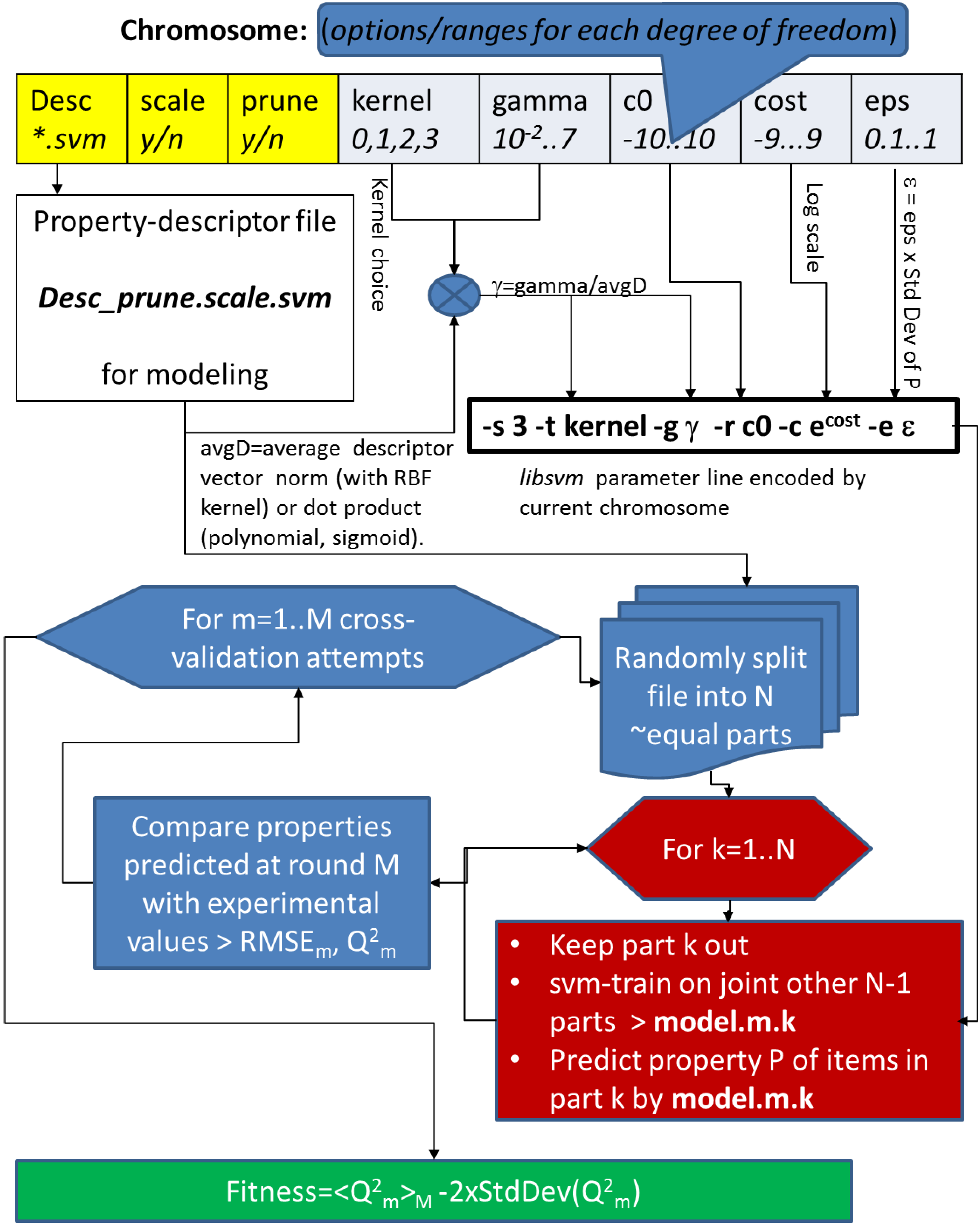
The syntax of .rng files is straightforward. Column one designs the name of the degree of freedom defined on the current line. If this degree of freedom is categorical, the remaining fields on the line enumerate the values it may take. For example, line #1 is a list of descriptor spaces (including their optimally generated “pruned” versions) found in the working directory. The parameter “scale” chooses whether those descriptors should be used in their original form, or after Min/Max scaling (in clear, if scale is “orig”, then DS.orig.svm will be used instead of DS.scaled.svm). The “kernel” parameter picks the kernel type to be used with libsvm. Albeit a numeric code is used to define it on the svm-train command line (0—linear, 1—3rd order polynomial, 2—Radial Basis Function, 3—Sigmoid), on the .rng file line, the options were prefixed by “k” in order to let the soft handle this as a categoric option. The “ignore-remaining” keyword on the kernel line is a directive to the GA algorithm to ignore the further options and if the linear kernel choice k0 is selected. This is required for population redundancy control: two chromosomes encoding identical choices for all parameters except and do stand for genuinely different parameterization schemes, leading to models of different quality, unless the kernel choice is set to linear, which is not sensitive to and choices, leading to exactly the same modeling outcome. All .rng file lines having a numeric entry in column #2 are by default considered to encode continuous (discretized) variables. Such lines must obligatorily have 6 fields (besides #-marked comments): variable name, absolute minimal value, preferred minimal value, preferred maximum, absolute maximum and, last, output format definition implicitly controlling its precision. The distinction between absolute and preferred ranges is made in order to allow the user to focus on a narrowest range assumed to contain the targeted optimal value, all while leaving an open option for the exploration of larger spaces: upon random initialization or mutation of the variable, in 80% of cases the value will be drawn within the “preferred” boundaries, in 20% of cases within the “absolute” boundaries. The brute real value is then converted into a discrete option according to the associated format definition in the last column; it is converted to a string representation using sprintf(“<format representation>”, value), thus rounded up to as many decimal digits as mentioned in the decimal part of its format specifier. For example, the cost parameter spanning a range of width 18, with a precision of 0.1 may globally adopt 180 different values. Modifying the default “4.1” format specifier to “4.2” triggers a 10-fold increase of the phase space volume to be explored, in order to allow for a finer scan of cost.
2.2.5. The Genetic Algorithm
A chromosome will be rendered as a concatenation of the options picked for every parameter, in the order listed in the .rng file. They are generated on-the-fly, during the initialization phase of slave jobs, and not in a centralized manner. When the pilot submits a slave job, it does not impose the parameter configuration to be assessed by the slave, but expects the slave to generate such a configuration, based on the past history of explored configurations, and assess its goodness. In other words, this GA is asynchronous. Each so-far completed slave job will report the chromosome it has assessed, associated to its fitness score, by concatenation to the end of the done_so_far file in the working directory. The pilot script, periodically waking up from sleep to check the machine work load, will also verify whether new entries were meanwhile added to done_so_far. If so, it will update the population of so-far best, non redundant results in the working directory file best_pop, by sorting done_so_far by its fitness score, then discarding all chromosomes that are very similar to slightly fitter essays and cutting the list off at fitness levels of 70% of the best-so-far encountered fitness score (this “Darwinian selection” is the job of awk script $GACONF/chromdiv.awk).
A new slave job will propose a novel parameter configuration by generating offspring of these “elite” chromosomes in best_pop. In order to avoid reassessing an already seen, but not necessarily very fit, configuration, it will also read the entire done_so_far file, in order to verify that the intended configuration is not already in there. If so, genetic operators are again invoked, until a novel configuration emerges. However, neither best_pop nor done_so_far do not yet include configurations that are currently under evaluation on remote nodes. The asynchronous character of the GA does not allow absolute guarantees that it will be a perfectly self-avoiding search, albeit measures have been taken in this sense.
Upon lecture of best_pop and done_so_far, the parameter selector of the slave job (awk script $GACONF/make_childrenX.awk) may randomly decide (with predefined probability) to perform a “cross-over” between two randomly picked partners from best_pop, a “mutation” of a randomly picked single parent, or a “spontaneous generation” (random initialization, ignoring the “ancestors” in best_pop). Of course, if best_pop does not contain at least two individuals, the cross-over option is not available, and if best_pop is empty, at the beginning of the simulation, then the mutation option is unavailable as well: initially, all parameter configurations will be issued by “spontaneous generation”.
2.2.6. Slave Processes: Startup, Learning Steps, Output Files and Their Interpretation
Slave jobs run in temporary directories on the local file system of the nodes. A temporary directory is being assigned an unambiguous attempt ID, appended to its default name “attempt”. If the slave job successfully completes, this attempt folder will be, after cleaning of temporary files, copied back to the working directory. $GACONF also contains a sample working directory D1-workdir, displaying typical results obtained from regression-based learning from D1-datadir; you may browse through it in order to get acquainted with output files. The attempt ID associated to every chromosome is also reported in the result file done_so_far. Inspect $GACONF/D1-workdir/done_so_far. Every line thereof is formally divided by an equal sign in two sub-domains. The former encodes the actual chromosome (field #1 stands for chosen DS, #2 for the descriptor scaling choice, ...). Fields at right of the “=” report output data: attempt ID, fitting score and, as last field on line, the XV fitness score, for regression, for classification problems as defined in Introduction. The fitting score is calculated, for completeness, as the “mean-minus-two-sigma” of fitted correlation coefficients and fitted balanced accuracy. Please do not allow yourself to be confused by “fitting” (referring to statistics of the svm-train model fitting process, and concerning the instances used to build the model), and Darwinian “fitness” (defined on the basis of XV results). The fitting score is never used in the Darwinian selection process; it merely serves to inform the user about the loss of accuracy between fitted and predicted/cross-validated property values.
IMPORTANT! Since every slave job will try to append its result line to done_so_far as soon as it has completed calculations, chance may have different jobs on different nodes, each “seeing” the working directory on a NFS-mounted partition, attempt to simultaneously write to done_so_far. This may occasionally lead to corrupted lines, not matching the description above. Ignore them.
Yet, before results are copied back to the working directory, the actual work must be performed. This begins by generating a chromosome, unless the use_chromo option instructs the job to apply an externally imposed setup. After the chromosome is generated and stored in the current attempt folder, it first must be interpreted. On one hand, the chromosome contains descriptor selection information. The property-descriptor matrix matching the name reported in the first field of the chromosome, and more precisely its scaled or non-scaled version, as indicated by the second field, will be the one copied to the attempt folder, for further processing. The remaining chromosome elements must be translated into the actual libsvm command line options. In this sense, the actual ϵ value for regression is calculated by multiplying the epsilon parameter in the chromosome by the standard deviation of the training property values. In this way, ϵ, representing 10 to 100% of the natural deviation of the property, implicitly has the proper order of magnitude and proper units. Likewise, the chromosome gamma parameter will be converted to the actual value, dividing by the mean vector dot product (for kernel choices k1 or k3), or by the mean Euclidean distance (kernel choice k2), respectively. Since the cost parameter is tricky to estimate, even in terms of magnitude orders, the chromosome features a log-scale cost parameter, to be converted into the actual cost by taking the exponential thereof. This, and also the stripping off of the “k” prefix in the kernel choice parameter, are also performed at the chromosome interpretation stage, mode-dependently carried out by dedicated “decoder” awk scripts chromo2SVMreg.awk and chromo2SVMclass.awk, respectively. At the end, the tool creates, within the attempt folder, the explicit option line required to pilot svm-train according to the content of the chromosome. This option line is stored in a one-line file svm.pars; check out, for example, $GACONF/D1-workdir/attempt.11118/svm.pars, the option set that produced the fittest models so-far.
A singled-out property-descriptor matrix and a command-line option set for svm-train are the necessary and sufficient prerequisites to start XV. For each of the ntrials requested XV attempts, the order of lines in the property-descriptor matrix is randomly changes. The reordered matrix is then split into the requested lo folds. XV is explicit, and is not using the own facility of svm-train. Iteratively, svm-train is used to learn a local model on the basis of all but the left-out fold. If adding of decoys is desired, random decoy descriptor lines (of the same type, and having undergone the same scaling strategy as training set descriptors) are added to make up 50% of the local learning set size (the lo-1 folds in use). These will differ at each successive XV attempt, if the pool of decoys out of which they are drawn is much larger than the required half of training set size).
These local models are stored, and used to predict the entire training set, in which, however, the identities of local “training” and locally left-out (“test”) instances are known. These predictions are separately reported into “train” and “test” files. The former report, for each instance, fitted property values by local models having used the instance for training. The latter report predicted property values by local models not having used it for training.
Quality of fit is checked on-the-fly, and failure to exceed a predefined fitting quality criterion triggers a premature exit of the slave job, with a fictitious low fitness score associated to the current chromosome; see the fit_no_go option. In such a case, the attempt subdirectory is deleted, and a new slave job is launched instead to the defunct one.
Results in the attempt subdirectories of D1-workdir correspond to the default 12 times repeated leave-1/3-out XV schemes. This means that local models are generated. For each D1 ligand, there are exactly 12 of these local models that were not aware of that structure when they were fitted, and 24 others that did benefit from its structure-property information upon building.
Files final_train.pred.gz in attempt subdirectories (provided as compressed .gz) report, for each instance, the 24 “fitted” affinity values returned by models having used it for fitting (it is a 26-column file, in which column #1 reports current numbering and #2 contains the experimental affinity value). Reciprocally, the 14-column files final_test.pred.gz report the 12 prediction results stemming from models not encountering instances at fitting stage. Furthermore, consens_train.pred.gz and consens_test.pred.gz are “condensed” versions of the previous, in which the multiple predictions per line have been condensed to their mean (column #2) and standard deviations (column #3), column #1 being the experimental property.
Eventually, the stat file found in each attempt subdirectory provides detailed statistics about fitting and prediction errors in terms of root-mean-squared error, maximal error and determination coefficients. In a classification process, correctly classified fractions and balanced accuracies are reported. Lines labeled “local_train” compare every fitted value column from final_train, to the experimental data, whilst “local_test” represent local model-specific XV results. By extracting all the lines “local_test:r_squared”, actually representing the XV coefficients of every local model, and calculating the mean and standard deviations of these values, one may recalculate the fitness score of this attempt. The stat file lines labeled “test” and “train” compare the consensus means as reported in the consens_*.pred files to the experiment. Note: the determination coefficient “r_squared” between the mean of predictions and experiment tends to exceed the mean of local determination coefficients, reporting individual performances of local models. This is the “consensus” effect, not exploited in fitness score calculations that rely on the latter mean of individual coefficients, penalized by twice their standard deviations.
Last but not least, this model building exercise had included an external prediction set of D5 ligands, for which the current models were required to return a prediction of their D1 affinities. External prediction is enabled as soon as model fitness exceeds the user-defined threshold minlevel. This was the case for the best model corresponding to $GACONF/D1-workdir/attempt.11118/. External prediction file names are a concatenation of external set name (“D5”), the locally used DS (“treePH03_pruned”), the descriptor scaling status (“scaled”) and the extension “.pred”. As all these external items are, by definition, “external” to all the local models (no checking is performed in order to detect potential overlaps with the training set), the 38-column external prediction file will report the current numbering (column #1), the data reported in the first field of the .psvm files in column #2 (here, the experimental D5 values), followed by 36 columns of individual predictions of the modeled property (the D1 affinity values), by each of the local models. Since the external prediction set .psvm files had been endowed with numeric data in the first field of each line, the present tool assumes these to be corresponding experimental property values, to be compared to the predictions. Therefore, it will take the consensus of the 36 individual D1 affinity predictions for each item, and compare them to the experimental field. The results of external prediction challenge statistics are reported in the extval file of the attempt subdirectory. First, the strictest comparison consists in calculating the RMSE between experimental and predicted data, and the determination coefficient; these results are labeled “Det” in the extval report. However, external prediction exercises may be challenging, and sometimes useful even if the direct predicted-experimental error is large. For example, predicted values may not quantitatively match experiment, but happen to be all offset by a common value or, in the weakest case, nevertheless follow some linear trend, albeit of arbitrary slope and intercept. In order to test either of these hypotheses, extval also reports statistics for (a) the predicted vs. experimental regression line at fixed slope of 1.0, but with free intercept, labeled “FreeInt”, and (b) the unconstrained, optimal linear predicted-experimental correlation that may be established, labeled “Corr”.
In this peculiar case, extval results seem unlikely to make any sense, because the tool mistakenly takes the property data associated to external compounds (D5 affinities) for experimental D1 affinities, to be confronted with their predicted alter-egos. Surprise, even the strict Determination statistics are robustly positive on the fact that predicted D1 values quantitatively match experimental D5 values. This is due to the very close biological relatedness of the two targets, which do happen to share a lot of ligands. Indeed, 25% of the instances of the D5 external set were also reported ligands of D1, and, as such, part of the model training set. Yet, 3 out of 4 D5 ligands were genuinely new. This notwithstanding, their predicted D1 affinities came close to observed D5 values: a quite meaningful result confirming the extrapolative prediction abilities of the herein built model.
At this point, local SVM models and other temporary files are deleted, the chromosome associated to it attempt ID, fitting and fitness scores is being appended to done_so_far, and the attempt subfolder now containing only setup information and results is moved from its temporary location on the cluster back to the working directory (with exception of the workstation-based implementation, when temporary and final attempt subdirectory location are identical). The slave job successfully exits.
2.2.7. Reconstruction and Off-Package Use of Optimally Parameterized libsvm Models
As soon as the number of processed attempts reaches maxconfigs, the pilot script stops rescheduling new slave jobs. Ongoing slave processes are allowed to complete; therefore, the final number of lines in d one_so_far may slightly exceed maxconfigs. Before exiting, the pilot will also clean the working directories, by deleting all the attempt sub-folders corresponding to the less successful parameterization schemes, which did not pass the selection hurdle and are not listed in best_pop. A trace of their statistical parameters is saved in a directory called “losers”.
The winning attempt sub-folders contain all the fitted and cross-validated/predicted property tables and statistics reports, but not the battery of local SVM models that served to generate them. These were not kept, because they may be quite bulky files which may not be allowed to accumulate in large numbers on the disk (at the end of the run, before being able to decide which attempts can be safely discarded, there should have been maxconfigs × lo ntrials of them). However, they, or, actually, equivalent (recall that local model files are tributary to the random regrouping of kept vs. left-out instances at each XV step), model files can be rebuilt (and kept) by rerunning the pilot script with the use_chromo option pointing to a file with chromosomes encoding the desired parameterization scheme(s). If use_chromo points to a multi-line file, the rebuilding process may be parallelized: as the slave jobs proceed, new attempt sub-folders (now each containing lo ntrials libsvm model files) will appear in the working directory (but not necessarily in the listing order of use_chromo).
IMPORTANT! The file of preferred setup chromosomes should only contain the parameter fields, but not the chromosome evaluation information. Therefore, you cannot use
best_pop per se, or
‘head -top‘ of
best_pop as
use_chromo file, unless you first remove the right-most fields, starting at the “equal” separator:
head -top best_pop| sed ’s/=.*//’ > my_favorite_chromosomes.lst
$GACONF/pilot_<scheme>.csh workdir=<working directory used for GA
run> use_chromo=my_favorite_chromosomes.lst
Randomness at learning/left-out splitting stages may likely cause the fitness score upon refitting to (slightly) differ from the initial one (on the basis of which the setup was considered interesting). If the difference is significant, it means that the XV strategy was not robust enough; i.e., was not repeated sufficiently often (increase ntrials).
Local model files can now be used for consensus predictions, and the degree of divergence of their prediction for an external instance may serve as prediction confidence score [
7]. Remember that
svm-predict using those model files should be called on preprocessed descriptor files, as outlined in the Command-Line Launch subsection.
Alternatively, you may rebuild your libsvm models manually, using the svm-train parameter command line written out in successful attempt sub-folders. In this case, you may tentatively rebuild the models on your brute descriptor files, or on svm-scale-preprocessed descriptor files, unless the successful recipe requires pruning.


