Local Patch Vectors Encoded by Fisher Vectors for Image Classification

Abstract

The objective of this work is image classification, whose purpose is to group images into corresponding semantic categories. Four contributions are made as follows: (i) For computational simplicity and efficiency, we directly adopt raw image patch vectors as local descriptors encoded by Fisher vector (FV) subsequently; (ii) For obtaining representative local features within the FV encoding framework, we compare and analyze three typical sampling strategies: random sampling, saliency-based sampling and dense sampling; (iii) In order to embed both global and local spatial information into local features, we construct an improved spatial geometry structure which shows good performance; (iv) For reducing the storage and CPU costs of high dimensional vectors, we adopt a new feature selection method based on supervised mutual information (MI), which chooses features by an importance sorting algorithm. We report experimental results on dataset STL-10. It shows very promising performance with this simple and efficient framework compared to conventional methods.

1. Introduction

In recent years, image classification has been an active and important research topic in the field of computer vision and machine learning applications, e.g., image and video retrieval [1], biometrics [2], web content analysis [3] and video surveillance [4], etc. A standard pipeline to describe an image for image classification, is to extract a set of local descriptors, encode them into a high dimensional vector and pool them into an image-level signature. The feature extraction part is commonly accomplished by a wide spectrum of different local or global descriptors, like the well-known SIFT [5], SURF [6], HOG [7], LBP [8] and the recently proposed LIOP [9] and KAZE [10]. Although these hand-crafted features lead to reasonable results in various applications, they are only suitable for a particular data type or research domain and would result in dismal performance for other unknown usages [11]. Besides, designing a local descriptor is based on expert knowledge and experience. The cost of running an image detector per category is quite high [12]. Recently, there is a growing consensus that it is an alternative approach to utilize deep learning methods to obtain machine-learned features for image classification. Convolutional neural networks (CNN) is the most widely-used approach of deep learning methods. Due to the computational resources massively improved by GPU implementations and distributed computing clusters, deep CNNs have achieved remarkably high performance by surpassing the hand-crafted features on many visual recognition tasks [13]. In practice, there are some CNN models (e.g., Zeiler and Fergus [14] and Gao et al. [15]) popularly used as the deep feature extractor in image related tasks. In [15], the authors further happily combines the extracted CNN features and FV. Their work is based on the pre-trained CNN released by [16] (i.e., VGG Net-D). The number of parameters for this configuration is 138 M (here ‘M’ denotes million). Besides, training this architecture took 2–3 weeks depending on a system equipped with four NVIDIA Titan Black GPUs. Chandrasekhar et al. [17] combine CNN descriptors with FV for image instance retrieval. In [17], they consider four different pre-trained CNN models: OxfordNet, AlexNet, PlacesNet and HybridNet, with 138 M, 60 M, 60 M and 60 M parameters respectively. Although these promising results are presented in these publications to demonstrate the potential benefits of the deep CNNs, these models require numerous parameters to be tuned via iterative operations through layers; therefore, their computational cost is immense. Besides, learning such deep CNN networks useful for image classification critically depends on some ad hoc tricks. In recent years, the computational cost has become a central issue in object detection/image classification [12]. Most existing image classification methods use computationally expensive feature extraction, which is a very limiting factor considering the huge amount of data to be processed.

Aggregation of local features has been widely used to realize the task of classification or retrieval of 2D images. Our work is based on the FV feature encoding approach. The basic conception of this work is that a set of local image patches are sampled using several methods (e.g., randomly, densely, or using a key-point detector) and then each independent patch is evaluated to a vector of visual descriptor. The sampler is a critical part, which should focus attention on the image regions that are the most informative for classification. Within the Bag of Words (BOW) framework, Jurie and Triggs in [18] and Nowak et al. [19] show that sampling many different patches using either a regular dense grid [18] or a random strategy [19] works better than using interest points [20]. Hu et al. [21] divide the existing sampling methods into two types: random sampling and saliency-based sampling, and embed them in the BOW framework for scene classification of high-resolution remote sensing images. Although these authors investigate and quantitatively compare different sampling strategies in detail in their work, it is still not clear which sampling strategy is suitable for natural images under FV framework.

In this paper, instead of working towards more complex models, we focus on the local descriptors and their FV encoding. We will adopt raw image patches as local descriptors directly, which is simple, yet, is sufficiently efficient for image classification. Here, the term “efficient” refers to the relatively lower cost and complexity of applying raw image patches as local descriptors. It will reduce the complexity of the process of feature extraction and improve computing efficiency. For patch sampling strategy, we refer to the three methods as sparse sampling, dense sampling and saliency-guided sampling, and we investigate the effects of three different methods. Building on these advances, this paper proposes to combine FV with raw image patch vectors adapted to the representation of images, and to use the resultant representation to describe images. In order to embed both global and local spatial information into local features, we refine an existing spatial geometry structure which shows good performance. Finally, we address high dimensionality using a feature selection method called supervised MI based importance sorting algorithm; this was proposed by [22].

The paper is organized as follows: After introducing the proposed approach in Section 2, Section 3 shows the overall image classification framework and Section 4 gives the details of experiments and compares them with relevant literature. Section 5 elaborates on the conclusion of the study with a summary.

2. Description of the Proposed Approach

2.1. Constructing Local Patch Vectors

We now give the implementation details of constructing local patch vectors by extracting image patches. Patch sampling consists of selecting a compact but representative sub set of images. Given an image, we may use different sampling methods (e.g., saliency-based sampling, or random strategies) to select a set of local image patches, which can form a representative and informative subset of the image. The comparative studies [19,21,23] are devoted to these different sampling methods, which have a great influence on the results. Hence, this step is also the first and key part of our work.

We first extract large quantities of small patches in training images. Note that each patch has dimension r-by-r and has c channels (for natural images, there are only R, G, B channels), so each r-by-r patch can be represented as a vector in ${ℝ}^n$ of pixel intensity values, with n = r·r·c. For concreteness, the raw training image patch vectors can be denoted as ${\{x^{\left(i\right)}\in {ℝ}^n\}}_{i=1,\dots ,N}$, where N is the number of patches. So, our base representation of an image is as a set of local patch vectors. Before running a learning algorithm on our input data $x^{\left(i\right)}$, it is useful to pre-process these image patch vectors. That is, for each dimension of $x^{\left(i\right)}$, we subtract out the mean of its corresponding dimension and divide by the standard deviation. A small value is added to the variance before division to avoid dividing by zero.

We also considered zero component analysis (ZCA) whitening in this stage. In preliminary experiments (results not shown), we found that not using ZCA was more effective, and we did not use it in all of our experiments. The local patch vectors are Principal Component Analysis (PCA)-projected to reduce their dimensionality and to de-correlate their coefficients. PCA is usually applied to the SIFT features or fully connected layer activations, since it is empirically shown to improve the overall recognition performance. As the FV size scales linearly with feature dimension, using PCA can decrease the storage requirements and speed up the FV computation. De-correlating the data can make the data better fit the diagonal covariance assumption for Gaussian components. Finally, these vectors are power and L2-normalized to improve Fisher vector representation. In the above process, patch sampling strategies are most worth noting.

Patch sampling strategies The idea of representing images as collections of independent local patches has proved its worth for image classification or object recognition, but raises the issue of which patches to choose [19]. We investigate this question mainly by comparing three patch sampling strategies. Random: local patches are selected randomly in the spatial domain of the image. This means that every patch has the same probability to be sampled to represent the image content; all the patches are regarded to be equal. Dense: local patches are sampled evenly across the image on a dense grid with certain pixel spacing. This sampling strategy (processing every pixel of the image) captures the most information, but it is also computation and memory intensive, with much of the computation being spent on processing relatively featureless (and hence possibly uninformative) regions [19]. Saliency-based: Ideally, the sampler should focus attention on the image regions that are the most informative for classification [19]. This sampling strategy is inspired by attention mechanisms in the human visual system. Recently, selective attention models have drawn a lot of research attention [24,25]. The idea in selective attention is that not all parts of an image give us information. If we attend only to the relevant parts, we can recognize the image more quickly while using less resources [24]. An image’s visual saliency map can be used as a weighting function to indicate the importance of a local region to the human visual system [26]. In our work, we adopt the idea in [27] to obtain a visual saliency map, which has been proved to be effective, simple, and can generate excellent results in most cases. An image from the STL-10 dataset and its corresponding visual saliency map are illustrated in Figure 1.

Here the image’s visual saliency maps are used as masks to guide sampling: the brighter the region, the more likely it is to be sampled from the image. With respect to sampling patches, [21] sorts the values in a response map of every image in descending order and selects the first s proportion as the sampled points. Afterward, the patches centered on the sampled points are chosen as the representative set. In this paper, we adopt a more reasonable and preferable method proposed by [26]. Because the points of the visual saliency play a tiny role in human perception of the image quality, we choose the patches of which the mean visual saliency is not so small. Subsequently, given an image, we randomly sample N patches of which the mean visual saliency is larger than a threshold.

2.2. The Fisher Vector

In this section, we introduce the FV framework for image classification. Supposing that we are given an image, let $M=\{m_t,t=1,\dots N\}$ be the set of N local descriptors that are already extracted from it. The key idea of FV [28] is to model the generation process of local descriptors M by a probability density function $p(·;\theta )$ with parameters θ. The gradient (i.e., ${\nabla }_{\theta }\log p\left(M\right|\theta )$) of the log-likelihood with respect to the parameters of the model can describe how that parameter contributes to the generation process of M [29]. We usually model the probability density function by a Gaussian mixture model (GMM) using Maximum Likelihood (ML) estimation. Besides, $\theta =\{{\pi }_1{,\mu }_1{,\sigma }_1{,\dots \pi }_K{,\mu }_K{,\sigma }_K\}$ are the model parameters denoting the mixture weights, means, and diagonal covariance matrices of GMM, and K is the number of Gaussian components. After obtaining the GMM, image representations are computed using FV, which has been demonstrated to outperform the BoW model by a wide margin [30] and is a powerful method for aggregating local descriptors.

Let $G_{\mu ,k}^M$ and $G_{\sigma ,k}^M$ be the gradients with respect to ${\mu }_k$ and ${\sigma }_k$ of the component k. They can be computed using the following derivations:

$$G_{\mu ,k}^M=\frac{1}{N\sqrt{{\pi }_i}}{\displaystyle \sum _{t=1}^N{\gamma }_t(k)}\left(\frac{m_t-{\mu }_k}{{\sigma }_k}\right)$$

(1)

$$G_{\sigma ,k}^M=\frac{1}{N\sqrt{2{\pi }_i}}{\displaystyle \sum _{t=1}^N{\gamma }_t(k)}[\frac{{(m_t-{\mu }_k)}^2}{{\sigma }_k{}^2}-1]$$

(2)

where ${\gamma }_t\left(k\right)$ is the weight of local feature $m_t$ for the k-th Gaussian:

$${\gamma }_t(k)=\frac{{\pi }_k{\mu }_k(m_t)}{{\displaystyle {\sum }_{j=1}^K{\pi }_j{\mu }_j(m_t)}}$$

(3)

The final fisher vector is the concatenation of all $G_{\mu ,k}^M$ and $G_{\sigma ,k}^M$, which is a 2Kd-dimensional super vector, and d is the dimension of local feature m_t. In practice, the m_t in FV is usually not a raw local feature vector. Dimension reduction techniques are often first applied to the raw local features. Furthermore, PCA is usually used, because PCA has been proved beneficial for the success of FV [30].

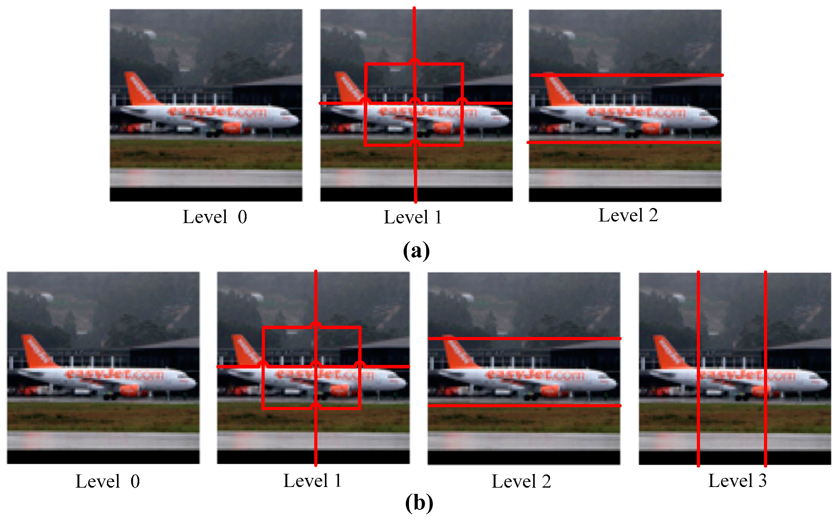
2.3. Incorporating Spatial Information

For successfully applying the important spatial information into FV image representation, we propose a new spatial pyramid matching structure. The main spatial pyramid approach (repeatedly sub-dividing the image into increasingly finer sub-regions by doubling the number of divisions on each axis direction) usually improves recognition by integrating correspondence results in these regions. It is straightforward to build a new one for our method. As shown in Figure 2a, the spatial regions are obtained by dividing the image in 1 × 1, 3 × 1 (three horizontal stripes), and 2 × 2 (four quadrants) grids pulsing a center block, for a total of 9 regions. We compute one encoding for each spatial region and then stack the results. Note that each spatial region is normalized individually prior to stacking.

In our experiment, we have also developed another spatial pyramid structure, which is depicted in Figure 2b. We add three vertical stripes in level 4 based on the former. Such structure does not improve the performance on the STL-10 dataset, but leads to increased memory consumption and computation time. Furthermore, it increases the dimension and storage of the final feature representation.

The reason for this could be that too finely subdivided levels resulting in individual bins yield too few matches when in a larger spatial structure level. This is also one of the limits of the spatial pyramid structure.

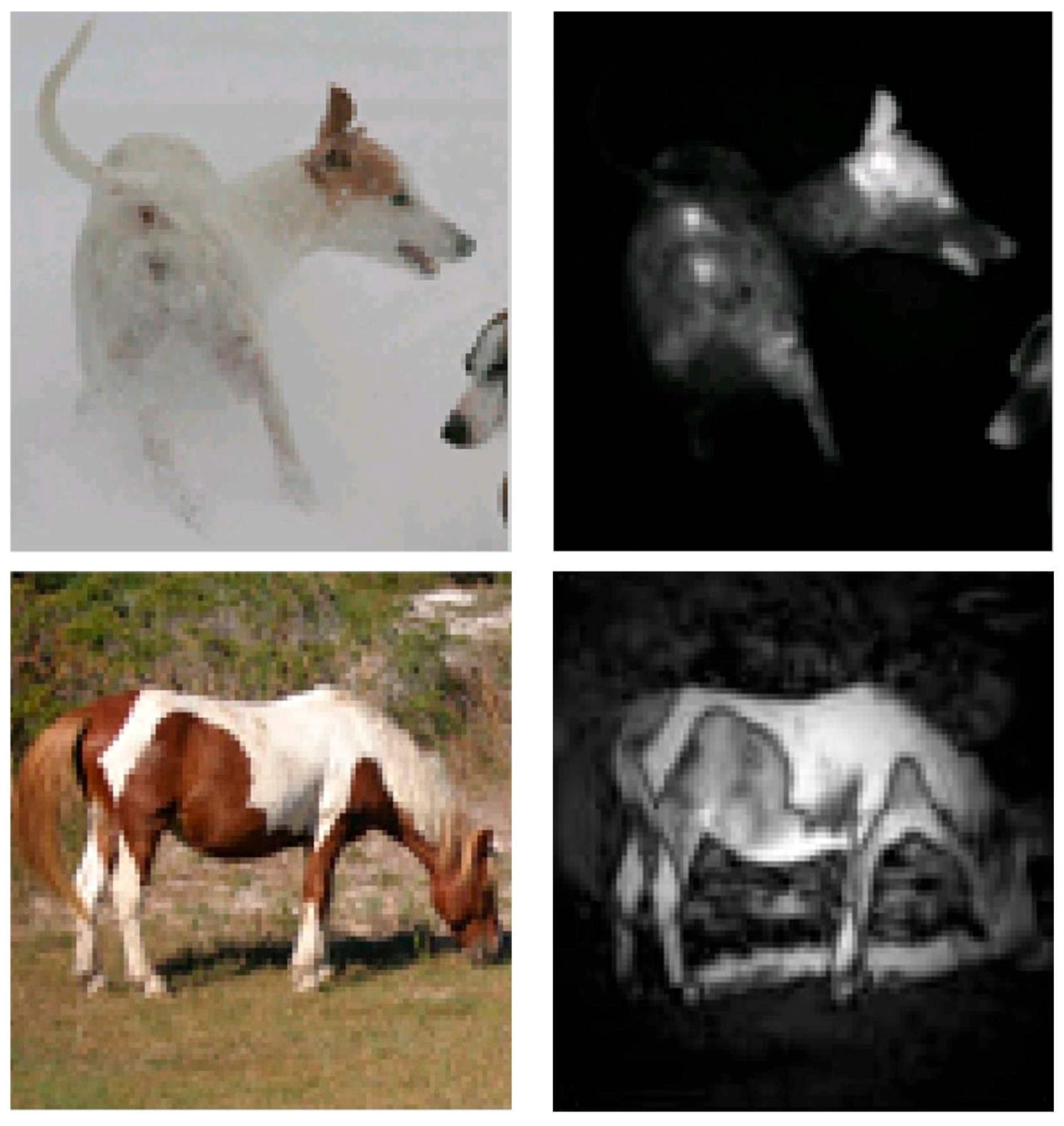
2.4. Feature Selection Based on MI

As previously discussed, the FV suffers from a disadvantage with respect to the BoW: while the latter is typically quite sparse, the FV is almost dense. This will lead to serious challenges for both feature vector storage and the subsequent classifier learning for image classification task. For this problem, feature compression has been proposed as a remedy, by compressing high dimensional feature vectors into feasible lengths. In [31], the authors divided these feature compression methods into three categories. The first category of these methods is Product Quantization (PQ) [12,32], which is a widely used feature compression method. The second are hashing based [33], which transform a real-valued feature vector into a shorter binary string. The last category transforms long vectors into shorter ones by using dimension reduction techniques. The authors [31] also proved that strong multi-collinearity may not exist among feature dimensions, which limits feature compression’s effectiveness and renders feature selection a better choice. Thus, we adopt a supervised mutual information (MI) based importance sorting algorithm to choose features, which is proposed in [31]. Specifically, we denote image labels as y, which we use to estimate how useful a single dimension is. We label the i-th dimension FV values as x_:i, and the mutual information as I(x_:i,y). The MI value is our importance score for each dimension, and can be computed as:

$$I\left(x_{\text{:}i},y\right)=H\left(y\right)+H\left(x_{\text{:}i}\right)-{H(x}_{\text{:}i},y)$$

(4)

where H is the entropy of a random variable. We just need to compute ${H(x}_{\text{:}i})-{H(x}_{\text{:}i},y)$ because y remains unchanged for different i. In [31], the authors use quantized discrete variables to compute entropy instead of estimating its probability distribution function by kernel density estimation. They also find that the 1-BIT quantization is better than 4-BINS and 8-BINS. We absorb this important observation in our work and use 1-bit quantization which quantizes a real number x into 2 discrete bins. The first bin (x ≥ 0) is stored as a value 1 in the bit, and the second bin (x < 0) is stored as a value 0.

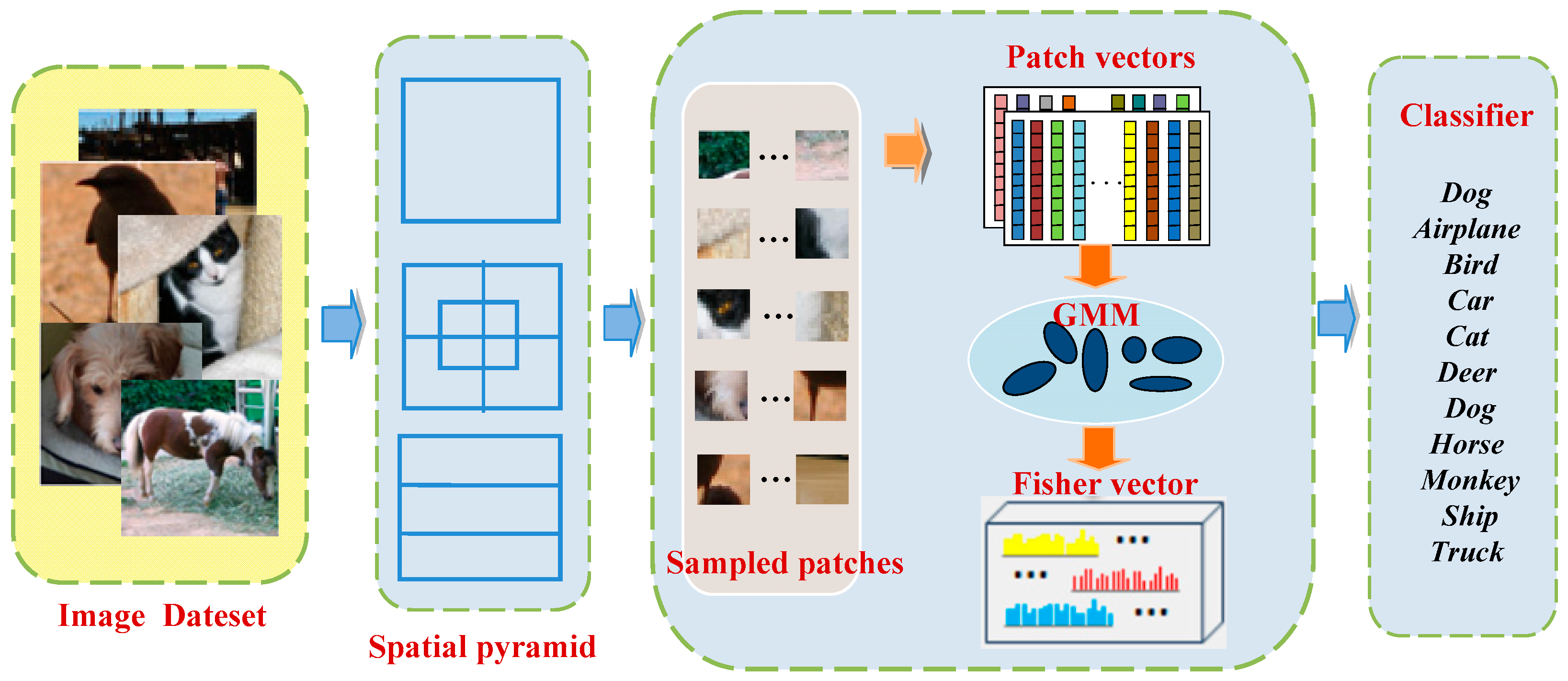
3. Image Classification Framework

The image classification flowchart based on our proposed method is depicted in Figure 3. To summarize, the whole image classification process can be mainly divided into five separate parts. These parts are, respectively:

• Extract patches. With the images as the input, the outputs of this step are image patches. This process is implemented via sampling local areas of images. Here we use three sampling manners (e.g., dense sampling using fixed grids, random sampling, and saliency-based sampling) to select a compact but representative subset of images. This step is the core part of our work.
• Represent patches. Given image patches, the outputs of this step are their feature vectors. We represent each image patch as a vector of pixel intensity values, and then pre-process these image patch vectors, subsequently, PCA is usually applied to these local patch vectors.
• Generate centroids. The inputs of this step are local image patch vectors extracted from all train images and the outputs are centroids. In our work, the centroids are generated by applying GMM over these local vectors. All centroids compose a discriminative codebook which can be used for feature encoding.
• Encode futures. In this step, the set of local feature descriptors are quantized with learned codebook of 64–512 centroids. For these features quantized to each centroid, we can aggregate first and second order residual statistics. Last, the final FV representation is obtained by concatenating the residual statistics from each centroid.
• Classification. This last step assigns a semantic class label to each image. This step usually relies on some trained classifier (e.g., SVM and soft-max). FV vectors are usually very high dimensional, especially in the case of employing the spatial pyramid structure. There exist many off-the-shelf SVM solvers, such as SVM^perf [34], or LibSVM/LIBLINEAR [35]. Limited by our main memory size, these are not feasible for such huge training features. Hence, in our work, we use the soft-max classifier for this discriminative stage.

4. Experiments

The purpose of this section is to evaluate the performance of our proposed complete classification pipeline. We first give the details of our implementation and baselines and then proceed to present and discuss the results on the STL-10 dataset. For the classification stage, soft-max classifier is used. Our experiments use the VLFeat [36] open source library to implement FV algorithms.

4.1. STL-10 Dataset

The STL-10 dataset is a natural image set for developing deep learning and unsupervised feature learning algorithms. It contains 10 classes: (1) airplane; (2) car; (3) bird; (4) cat; (5) dog; (6) deer; (7) horse; (8) monkey; (9) ship; and (10) truck with a resolution of 96 × 96. Figure 4 shows a few example images representing different classes that are included in this dataset. Each class has 500 training images and 800 testing images. The primary challenge is due to the smaller number of labeled training examples (100 per class for each training fold). We follow the standard setting in [37]: (1) train on each fold of 1000 examples and test on the full set of 8000 images; (2) report the average accuracy over the 10 folds and the standard deviation. An additional 100,000 unlabeled images are provided for unsupervised learning, which we do not use in our experiments, which is consistent with [37].

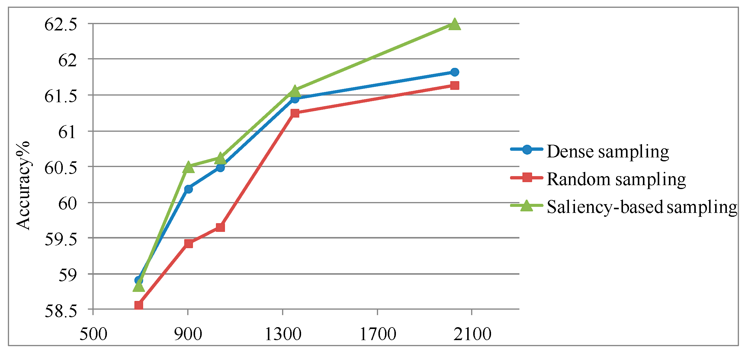
4.1.1. Evaluating the Sampling Performance

Patch sampling is the first and key procedure which has a great influence on the results. In this section, we focus on the effects of different sampling strategies mentioned above so as to find a suitable sampling strategy for the object classification of STL-10. For doing so, we fix the other procedures of the pipeline shown in Figure 3 but vary the sampling method, and measure the sampling performances by using the classification accuracy. This section also describes the default settings for our experimental studies. Besides, we discuss the impact of patch density and patch numbers on classification performance. With our implementation, we employ the SPR at pyramid level 0 (full image i.e., 1 × 1) for selecting a suitable sampling strategy. At this point, one of 10 folds samples are selected to train and the full set of 8000 images are for testing. At this pyramid level, the patch size tested is r = 8. For dense sampling, the patches are spaced by p pixels and q pixels on a regular grid in the direction of horizontal axis and vertical axis respectively. We can obtain the different numbers of sample patches by changing the values of [p, q] in pairs. According to the image resolution of STL-10, [p, q] are equipped as [3, 4], [3, 3], [2, 4], [3, 2] and [2, 2], respectively. Corresponding to these pairs, the numbers of patches sampled are as follows: 690, 900, 1035, 1350 and 2025. For fair comparison, we select the same number of patches based on saliency-based sampling and random sampling.

Supposing that we are given an image, the pixels of each patch are column reordered to form a vector in a r·r·c = 8 × 8 × 3 dimensional feature space. All of these vectors are packed into the columns of a matrix T motioned in Section 2.2. Then, for each m_t inside T, we perform the PCA. The threshold of PCA is chosen such that 99% energy is retained. After applying the L₂ vector normalization, we train a GMM with 256 centroids in all the experiments (unless stated otherwise). By default, for the FV computation, we only compute the gradients with respect to the mean and standard deviation parameters (but not the mixture weight parameters). In addition, the final FV $f_{\theta }\left(M\right)$ is improved by the power-normalization with the factor of 0.5, then followed by the L₂ vector normalization.

Figure 5 shows the results using different sampling methods. The horizontal axis indicates the numbers of sampled patches, and the vertical axis is classification accuracy with different sampling numbers. As shown in Figure 5, all the curves share the same properties: they are increasing in the general trend. This implies that the three sampling methods will give similar results when the information contained in the sampled patches is close to some extent. However, saliency-based sampling obviously outperforms others, except at 690. The next highest is dense sampling, which provides a very large number of feature patches. We can also learn from the results that, as the sampled numbers become larger, the differences between saliency-based sampling and the other two methods is even greater. This conclusion is different from [19,21], which come to the consistent conclusion that: random sampling is the best choice to improve the classification performance in high-resolution remote sensing imagery and natural images. In their conclusion, saliency-based sampling cannot compete with random sampling. We conclude that this is mainly due to the fact that key-point detectors are regarded as saliency-based sampling measures in their literature. In our work, we adopt the mean visual saliency of patches as a measure, which is more reasonable. In addition, it is clear that one of the main parameters governing classification accuracy is the number of patches used. Theoretically, the more patches that we sample from the images, the more accurate our method will be, but we find approximately 2000 patches are enough to catch sufficient information at pyramid level 0.

4.1.2. Main Results

According to the inference of Section 4.1.1, we apply the saliency sampling strategy to pyramid level 1, 2 again. We adopt the structure of pyramid level 1, 2 to divide saliency maps of the dataset. Please note that we compute one GMM for each spatial region and then the results of different blocks are concatenated to form the final representation. We extract 1500 and 2000 patches for every block of level 1 and 2 respectively. The same FV calculation process in Section 4.1.1 is also used for spatial regions of level 1 and 2. FV vectors are usually very high dimensional, e.g., when the number of centroids of GMM is set to 256, the total number of dimensions in FV is approximately 241,125 dimensions in this paper. Such high-dimensional features cause enormous memory storage and CPU time requirements. We apply the MI-based feature selection [31], which is much more effective than compression methods. The feature selection results with different selection ratios (c = 90%, 80%, 70%, 60%) are shown in

Table 1. Accuracy [%] of different selection ratios on 10 training folds. The rows labeled as “None” are the accuracy of the unselected feature. When a different selection ratio is compared with the baselines, a ↑ or ↓ sign indicates that the results of this selection ratio is better than or worse than the baseline; a = sign indicates that the results of this selection ratio is equal to the baseline. c means the selection ratio.

	Fold 1	Fold 2	Fold 3	Fold 4	Fold 5	Fold 6	Fold 7	Fold 8	Fold 9	Fold 10	Average Accuracy
None	67.94	68.03	66.78	67.39	66.86	67.06	67.09	65.56	67.79	67.41	67.19 ± 0.72
c = 90%	67.94=	68.19↑	66.65↓	67.55↑	66.65↓	66.94↓	66.94↓	65.78↑	67.88↑	67.30↓	67.18 ± 0.74
c = 80%	67.85↓	68.08↑	66.59↓	67.44↑	66.65↓	66.98↓	66.73↓	65.73↑	67.63↓	67.35↓	67.10 ± 0.71
c = 70%	67.76↓	67.88↓	66.43↓	67.39=	66.56↓	67.14↑	66.49↓	65.50↓	67.71↓	67.23↓	67.01 ± 0.75
c = 60%	67.56↓	67.43↓	65.99↓	67.35↓	66.59↓	66.89↓	66.38↓	65.59↑	67.54↓	67↓	66.83 ± 0.68

. For some folds of STL-10 (e.g., fold 9 and fold 10), the MI-based feature selection strategy can improve the baseline accuracy, although they only use 60% to 90% of the original feature dimensions in the baseline. The reason for this is that, many dimensions in the FV representation around these folds are noise and removing them will even improve classification accuracy. For overall average accuracy, choosing the selection ratio from 60% to 90%, the recognition accuracy degradation is also minuscule and gradual. This feature selection method that we used can improve the image classification performance required and reduce the computational cost for learning the classifier.

We also compared our proposed method with some off-the-shelf image classification methods that have reported recognition accuracy on the STL-10 dataset. We do not list the results of supervised methods on STL-10 (the best of which currently exceed 70% accuracy). As can be seen in

Table 2. Comparison of test accuracy mean ± std% on all folds of STL-10.

Method	Accuracy
Convolutional K-means Network [38] (2011)	60.1 ± 1.0
SCDAE 2 layer [39] (2017)	60.5 ± 0.9
Slowness on videos [40] (2012)	61.0
Sparse feature learning [41] (2014)	61.10 ± 0.58
View-Invariant K-means [42] (2013)	63.7
HMP [43] (2013)	64.5 ± 1
Stacked what-where AE [44] (2016)	74.33
Examplar CNN [45] (2014)	75.4 ± 0.3
Ours (c = 70%)	67.01 ± 0.75

, our results can be compared to and exceed the performance of many unsupervised algorithms on this dataset. More importantly, our method has no more meta-parameters that need to be tuned, compared with other algorithms (e.g., the meta-parameters required by [38] are weight decay, sparseness constant, sparsity penalty).

Here, we also discuss the classification rate of different spatial levels. The direct comparison is shown in

Table 3. Test accuracy mean ± std% over different spatial level.

Level	Level 0	Level 0–1	Level 0–2
Mean Accuracy	60.69 ± 0.7	66.53 ± 0.5	67.01 ± 0.75

. We can see that a substantial increase in performance can be obtained with the spatial level increase. To summarize, our method achieves satisfactory performance with few parameters tuning on STL-10 at a low computational cost.

5. Conclusions

This paper presents a simple image classification model, which directly adopts raw image patch vectors as local descriptors encoded by FV subsequently. This model appropriately compares and analyzes three typical sampling strategies: random sampling, saliency-based sampling and dense sampling. The final representation of each image is embedded spatial information, by constructing an improved spatial geometry structure. Finally, we adopt a MI-based feature selection method to choose features by importance sorting algorithm.

Experimental results show that our method based on local patch vectors and FV outperforms several unsupervised approaches on the STL-10 dataset. Besides, it is easy to implement. It has nearly no parameters to tune, and evaluates extremely fast. Meanwhile, it has the merits of low time and space complexities compared with previous unsupervised works.

References

1. Vailaya, A.; Figueiredo, M.A.T.; Jain, A.K.; Zhang, H.J. Image classification for content-based indexing. IEEE Trans. Image Process. 2001, 10, 117–130. [Google Scholar] [CrossRef] [PubMed]
2. Jain, A.K.; Ross, A.; Prabhakar, S. An introduction to biometric recognition. IEEE Trans. Circuits Syst. Video Technol. 2004, 14, 4–20. [Google Scholar] [CrossRef]
3. Kosala, R.; Blockeel, H. Web mining research: A survey. ACM Sigkdd Explor. Newsl. 2000, 2, 1–15. [Google Scholar] [CrossRef] [Green Version]
4. Collins, R.T.; Lipton, A.J.; Kanade, T.; Fujiyoshi, H.; Duggins, D.; Tsin, Y.; Tolliver, D.; Enomoto, N.; Hasegawa, O.; Burt, P. A System for Video Surveillance and Monitoring; VSAM Final Report; The Robotics Institute, Carnegie Mellon University: Pittsburgh, PA, USA, 2000; pp. 1–68. [Google Scholar]
5. Lowe, D.G. Distinctive image features from scale-invariant keypoints. Int. J. Comput. Vis. 2004, 60, 91–110. [Google Scholar] [CrossRef]
6. Bay, H.; Tuytelaars, T.; Gool, L.V. SURF: Speeded Up Robust Features. Comput. Vis. Image Underst. 2006, 110, 404–417. [Google Scholar]
7. Dalal, N.; Triggs, B. Histograms of oriented gradients for human detection. In Proceedings of the IEEE Computer Society Conference on Computer Vision and Pattern Recognition, San Diego, CA, USA, 21–23 September 2005; pp. 886–893. [Google Scholar]
8. Ahonen, T.; Hadid, A.; Pietikäinen, M. Face Recognition with Local Binary Patterns. In Proceedings of the European Conference on Computer Vision, Prague, Czech Republic, 11–14 May 2004; pp. 469–481. [Google Scholar]
9. Wang, Z.; Fan, B.; Wu, F. Local Intensity Order Pattern for feature description. In Proceedings of the International Conference on Computer Vision, Barcelona, Spain, 6–13 November 2011; pp. 603–610. [Google Scholar]
10. Alcantarilla, P.F.; Bartoli, A.; Davison, A.J. KAZE Features. In Proceedings of the European Conference on Computer Vision, Florence, Italy, 7–13 October 2012; pp. 214–227. [Google Scholar]
11. Yin, H.; Jiao, X.; Chai, Y.; Fang, B. Scene classification based on single-layer SAE and SVM. Expert Syst. Appl. 2015, 42, 3368–3380. [Google Scholar] [CrossRef]
12. Sánchez, J.; Perronnin, F.; Mensink, T.; Verbeek, J. Compressed Fisher Vectors for Large-Scale Image Classification; Research Report RR-8209; HAL-Inria: Rocquencourt, France, 2013. [Google Scholar]
13. Shi, H.; Zhu, X.; Lei, Z.; Liao, S.; Li, S.Z. Learning Discriminative Features with Class Encoder. In Proceedings of the IEEE Conference on Computer Vision and Pattern Recognition Workshops, San Francisco, CA, USA, 13–18 June 2016; pp. 46–52. [Google Scholar]
14. Zeiler, M.D.; Fergus, R. Visualizing and understanding convolutional networks. In Proceedings of the European Conference on Computer Vision, Zurich, Switzerland, 6–12 September 2014; pp. 818–833. [Google Scholar]
15. Gao, B.B.; Wei, X.S.; Wu, J.; Lin, W. Deep spatial pyramid: The devil is once again in the details. arXiv, 2015; arXiv:1504.05277. [Google Scholar]
16. Simonyan, K.; Zisserman, A. Very deep convolutional networks for large-scale image recognition. arXiv, 2014; arXiv:1409.1556. [Google Scholar]
17. Chandrasekhar, V.; Lin, J.; Morère, O.; Goh, H.; Veillard, A. A practical guide to CNNs and Fisher Vectors for image instance retrieval. Signal Process. 2016, 128, 426–439. [Google Scholar] [CrossRef]
18. Jurie, F.; Triggs, B. Creating Efficient Codebooks for Visual Recognition. In Proceedings of the IEEE International Conference on Computer Vision, Beijing, China, 17–21 October 2005; pp. 604–610. [Google Scholar]
19. Nowak, E.; Jurie, F.; Triggs, B. Sampling Strategies for Bag-of-Features Image Classification. In Proceedings of the European Conference on Computer Vision, Marseille, France, 12–18 October 2008; pp. 490–503. [Google Scholar]
20. Zhang, J.; Marszałek, M.; Lazebnik, S.; Schmid, C. Local Features and Kernels for Classification of Texture and Object Categories: A Comprehensive Study. Int. J. Comput. Vis. 2007, 73, 213–238. [Google Scholar] [CrossRef]
21. Hu, J.; Xia, G.S.; Hu, F.; Sun, H. A comparative study of sampling analysis in scene classification of high-resolution remote sensing imagery. In Proceedings of the Geoscience and Remote Sensing Symposium, Milan, Italy, 13–18 July 2015; pp. 14988–15013. [Google Scholar]
22. Zhang, Y.; Wu, J.; Cai, J. Compact Representation of High-Dimensional Feature Vectors for Large-Scale Image Recognition and Retrieval. IEEE Trans. Image Process. 2016, 25, 2407. [Google Scholar] [CrossRef] [PubMed]
23. Shi, F.; Petriu, E.; Laganiere, R. Sampling Strategies for Real-Time Action Recognition. In Proceedings of the Computer Vision and Pattern Recognition, Portland, OR, USA, 25–27 June 2013; pp. 2595–2602. [Google Scholar]
24. Salah, A.A.; Alpaydin, E.; Akarun, L. A selective attention-based method for visual pattern recognition with application to handwritten digit recognition and face recognition. IEEE Trans. Pattern Anal. Mach. Intell. 2002, 24, 420–425. [Google Scholar] [CrossRef]
25. Borji, A.; Itti, L. State-of-the-Art in Visual Attention Modeling. IEEE Trans. Pattern Anal. Mach. Intell. 2012, 35, 185–207. [Google Scholar] [CrossRef] [PubMed]
26. Gu, Z.; Zhang, L.; Li, H. Learning a blind image quality index based on visual saliency guided sampling and Gabor filtering. In Proceedings of the IEEE International Conference on Image Processing, Melbourne, Australia, 15–18 September 2013; pp. 186–190. [Google Scholar]
27. Zhang, L.; Gu, Z.; Li, H. SDSP: A novel saliency detection method by combining simple priors. In Proceedings of the IEEE International Conference on Image Processing, Paris, France, 27–30 October 2014; pp. 171–175. [Google Scholar]
28. Wu, J.; Yu, Z.; Lin, W. Good practices for learning to recognize actions using FV and VLAD. IEEE Trans. Cybern. 2016, 46, 2978–2990. [Google Scholar] [CrossRef] [PubMed]
29. Ma, B.; Su, Y.; Jurie, F. Local Descriptors Encoded by Fisher Vectors for Person Re-identification. In Proceedings of the European Conference on Computer Vision, Florence, Italy, 7–13 October 2012; pp. 413–422. [Google Scholar]
30. Sánchez, J.; Perronnin, F. Image Classification with the Fisher Vector: Theory and Practice. Int. J. Comput. Vis. 2013, 105, 222–245. [Google Scholar] [CrossRef]
31. Zhang, Y.; Wu, J.; Cai, J. Compact representation for image classification: To choose or to compress? In Proceedings of the IEEE Conference on Computer Vision and Pattern Recognition, Columbus, OH, USA, 24–27 June 2014; pp. 907–914. [Google Scholar]
32. Jégou, H.; Douze, M.; Schmid, C. Product quantization for nearest neighbor search. IEEE Trans. Pattern Anal. Mach. Intell. 2011, 33, 117–128. [Google Scholar] [CrossRef] [PubMed] [Green Version]
33. Sanchez, J.; Perronnin, F. High-dimensional signature compression for large-scale image classification. In Proceedings of the IEEE Conference on Computer Vision and Pattern Recognition, Colorado Springs, CO, USA, 20–25 June 2011; pp. 1665–1672. [Google Scholar]
34. Joachims, T. Training linear SVMs in linear time. In Proceedings of the 12th ACM SIGKDD International Conference on Knowledge Discovery and Data Mining, Philadelphia, PA, USA, 20–23 August 2006; pp. 217–226. [Google Scholar]
35. Fan, R.E.; Chang, K.W.; Hsieh, C.J.; Wang, X.R.; Lin, C.J. LIBLINEAR: A library for large linear classification. J. Mach. Learn. Res. 2008, 9, 1871–1874. [Google Scholar]
36. Vedaldi, A.; Fulkerson, B. VLFeat: An open and portable library of computer vision algorithms. In Proceedings of the 18th ACM International Conference on Multimedia, Firenze, Italy, 25–29 October 2010; pp. 1469–1472. [Google Scholar]
37. Miclut, B. Committees of deep feedforward networks trained with few data. In Proceedings of the German Conference on Pattern Recognition, Münster, Germany, 2–5 September 2014; pp. 736–742. [Google Scholar]
38. Coates, A.; Ng, A.Y. Selecting receptive fields in deep networks. In Proceedings of the Advances in Neural Information Processing Systems, Granada, Spain, 12–17 December 2011; pp. 2528–2536. [Google Scholar]
39. Du, B.; Xiong, W.; Wu, J.; Zhang, L.; Zhang, L.; Tao, D. Stacked convolutional denoising auto-encoders for feature representation. IEEE Trans. Cybern. 2017, 47, 1017–1027. [Google Scholar] [CrossRef] [PubMed]
40. Zou, W.Y.; Ng, A.Y.; Zhu, S.; Yu, K. Deep learning of invariant features via simulated fixations in video. In Proceedings of the Advances in Neural Information Processing Systems, Lake Tahoe, NV, USA, 3–6 December 2012; pp. 3203–3211. [Google Scholar]
41. Romero, A.; Radeva, P.; Gatta, C. No more meta-parameter tuning in unsupervised sparse feature learning. arXiv, 2014; arXiv:1402.5766. [Google Scholar]
42. Hui, K.Y. Direct modeling of complex invariances for visual object features. In Proceedings of the International Conference on Machine Learning, Atlanta, GA, USA, 16–21 June 2013; pp. 352–360. [Google Scholar]
43. Bo, L.; Ren, X.; Fox, D. Unsupervised feature learning for RGB-D based object recognition. In Proceedings of the 13th International Symposium on Experimental Robotics; Springer: Cham, Switzerland, 2013; pp. 387–402. [Google Scholar]
44. Zhao, J.; Mathieu, M.; Goroshin, R.; Lecun, Y. Stacked What-Where Auto-encoders. In Proceedings of the International Conference on Learning Representations, San Juan, Puerto Rico, 2–4 May 2016. [Google Scholar]
45. Dosovitskiy, A.; Springenberg, J.T.; Riedmiller, M. Discriminative unsupervised feature learning with convolutional neural networks. In Proceedings of the Advances in Neural Information Processing Systems, Montreal, QC, Canada, 8–13 December 2014; pp. 766–774. [Google Scholar]
Figure 1. Two images from STL-10 dataset and its corresponding visual saliency map computed by using the saliency model proposed in [27].
Information 09 00038 g001
Figure 2. Two Spatial Pyramid Representations (SPRs). (a) An improved spatial pyramid structure we proposed. (b) Another spatial pyramid structure we developed.
Information 09 00038 g002
Figure 3. The proposed image classification framework.
Information 09 00038 g003
Figure 4. Some example images of STL-10 dataset.
Information 09 00038 g004
Figure 5. Comparisons of classification accuracy using different sampling methods at pyramid level 0 of STL-10 dataset.
Information 09 00038 g005