Analyzing the MHD Bioconvective Eyring–Powell Fluid Flow over an Upright Cone/Plate Surface in a Porous Medium with Activation Energy and Viscous Dissipation

Abstract

In the field of heat and mass transfer applications, non-Newtonian fluids are potentially considered to play a very important role. This study examines the magnetohydrodynamic (MHD) bioconvective Eyring–Powell fluid flow on a permeable cone and plate, considering the viscous dissipation (0.3 ≤ E_c ≤0.7), the uniform heat source/sink (−0.1 ≤ Q₀ ≤ 0.1), and the activation energy (−1 ≤ E₁ ≤ 1). The primary focus of this study is to examine how MHD and porosity impact heat and mass transfer in a fluid with microorganisms. A similarity transformation (ST) changes the nonlinear partial differential equations (PDEs) into ordinary differential equations (ODEs). The Keller Box (KB) finite difference method solves these equations. Our findings demonstrate that adding MHD (0.5 ≤ M ≤ 0.9) and porosity (0.3 ≤ Γ ≤ 0.7) effects improves microbial diffusion, boosting the rates of mass and heat transfer. Our comparison of our findings to prior studies shows that they are reliable.

1. Introduction

Vertical cones and plate-shaped tools are frequently utilized in a variety of industries, including the processing of chemicals, food production, metal fabrication, casting facilities, and fabrics. Industrial operations often necessitate the prompt cooling of these tools after use. Vertical cone/plate mixers are essential in the production of high quality, safe items that are used globally, such as food, medications, and personal hygiene products. Every vertical cone/plate mixer model is meticulously crafted to fulfill distinct industrial objectives. Utilizing vertical cone or plate mixers leads to a discernible enhancement in grinding efficiency, causing the surface of the mixer to warm up on the cone and plate. The heating phenomenon arises due to the rapid and thorough mixing of the mixture, which facilitates the transfer of heat across the surface of the cone and plate. In this context, we focus on a specific category of non-Newtonian fluid known as Eyring–Powell fluid. In the current study, we investigate how microorganisms affect the processes of heat and mass transfer and provide methods for reducing these impacts by using magnetohydrodynamics (MHD) and porosity.

Non-Newtonian models for heat transfer and other applications have been widely analyzed [1,2,3,4,5]. The impact of MHD is crucial for heat transfer and has numerous engineering applications. Numerous studies have looked at the heat transfer of MHD fluids, especially with respect to Newtonian and non-Newtonian fluid flow over variations in geometries [6,7,8,9,10]. In the field of fluid dynamics and heat transfer, several noteworthy studies have been conducted. Muhammet Yurusoy [11] investigated the pressure distribution of a slider bearing lubricated with Eyring–Powell fluid. Barth and Carey [12] focused on benchmark problems involving natural convection using non-Newtonian fluids. Bapuji Pullepu et al. [13] examined the heat transfer characteristics of unsteady laminar natural convection flow over an isothermal vertical cone. In addition to their previous work, the researchers extended their investigation to analyze the phenomenon of unsteady laminar free convection from a vertical cone subjected to a uniform surface heat flux. Their objective was to gain a clearer understanding of the complex dynamics involved in heat transfer within this specific configuration [14]. Manisha Patel and Timol [15] conducted a numerical study on the laminar incompressible flow of a non-Newtonian fluid past a vertical wedge, with a specific emphasis on satisfying asymptotic boundary conditions. Additionally, they investigated the stress–strain relationship for viscoelastic non-Newtonian fluids through numerical analysis [16]. Raju et al. [17] addressed magnetohydrodynamic (MHD) nanofluid flow over a moving vertical plate. Macharla Jayachandra Babu et al. [18] explored the effects of thermophoresis and Brownian motion on the boundary layer flow of an MHD Eyring–Powell nanofluid over a permeable cone, considering buoyancy forces and suction/injection effects. Koriko et al. [19] analyzed the intricate interplay of thermal stratification, nonlinear thermal radiation, and quartic autocatalytic chemical reaction effects on the flow of a three-dimensional Eyring–Powell alumina–water nanofluid. Khan et al. [20] investigated the steady three-dimensional MHD flow of an Eyring–Powell nanofluid, considering convective and nanoparticles mass flux conditions as well as thermal radiation effects. Imad Khan et al. [21] investigated the boundary layer flow of an Eyring–Powell nanofluid over a plate and cone, considering chemically reactive species. Rehman et al. [22] and Simon et al. [23] employed the Lie symmetry integrative process to analyze the boundary layer flow of non-Newtonian fluid towards a flat porous surface, incorporating heat and concentration transfer along with free stream momentum. Waqas et al. [24] employed the Cattaneo–Christov model to non-Newtonian fluid. Navid Balazadeh et al. [25] explored heat and mass transfer in an unsteady two-dimensional squeezing flow of a non-Newtonian MHD radiative Eyring–Powell fluid, accounting for heat generation/absorption, thermal radiation, and Joule heating. Layek et al. [26] investigated the effects of various factors on unsteady non-Newtonian fluid flow over a widening sheet, while Sami Ullah Khan et al. [27] examined the influence of heat exposure, MHD, and poroelasticity on the movement of a non-Newtonian water-based nanofluid in different regions. Gaffar et al. [28] studied the flow and heat transfer of an Eyring–Powell micropolar fluid boundary layer over an upright non-isothermal cone. Khan et al. [29] analyzed the flow of a bioconvective nanofluid with temperature-dependent viscosity and surface pressure using a perpendicular plate. Oke [30] investigated the flow of an electrically conductive modified Eyring–Powell fluid utilizing a spinning surface and thermal radiation. Dania Qaiser [31] and her colleagues investigated the two-dimensional mixed convection stagnation point flow of nanofluid across a shrinking sheet. Xia et al. [32] focused on the effects of activation energy on bioconvective MHD non-Newtonian fluid flow on stretchable cylinders, providing insights into non-Newtonian fluid dynamics in biological contexts. Fatunmbi et al. [33] examined non-Newtonian fluid flow models for permeable Riga surfaces, incorporating thermal radiation and MHD effects. Habib et al. [34] explored the bioconvective fluid flow of three different non-Newtonian fluids on stretchable surfaces, considering the activation energy and dual diffusion. Baranovskii [35] studied the optimal boundary control of the Boussinesq approximation for polymeric fluids. The state functions for this problem are temperature and flow velocity, whereas the control function is the heat flux through a specified portion of the flow domain boundary. Farooq et al. [36] investigated nanofluid flows with different stress conditions using blood and magnesium nanoparticles on stretchable surfaces. El-Dabe and Mostapha [37] analyzed peristaltic blood flow with MHD and dual diffusion using the homotopy perturbation analytical method. Basha et al. [38] studied non-Newtonian fluid flow on circular cylinders, considering the effects of MHD. Khan et al. [39] examined the non-Newtonian fluid flow bioconvective model, incorporating MHD and Cattaneo–Christov heat flux conditions. Raghunath et al. [40] investigated natural convective fluid flow on vertical surfaces, taking into account thermal radiation effects. Bhattacharyya et al. [41] analyzed peristaltic blood flow with the Joule heating effect and MHD. Pasha et al. [42] numerically solved hybrid nanofluid flows on slippery surfaces using the finite element method. Shevchuk [43] investigated an analytical solution for the convective heat transfer in conical gaps with either a rotating cone or disc. Baranovskii [44] examined exact solutions for non-isothermal flows of second-grade fluid between parallel plates. These studies contribute to the understanding of fluid dynamics, heat transfer, and nanofluid behavior, enhancing our knowledge of these phenomena. Nisha and Poulomi [45] investigated Hall currents and the ion slip effect on Sisko nanofluid flow featuring chemical reaction over a porous medium applying a statistical approach.

Eyring–Powell fluid bioconvection flow on a vertical cone/plate surface has not yet been explored for mass and heat transfer dynamics. We consider several crucial elements that impact behavior, such as MHD, porous media, viscous dissipation, uniform heat source/sink, and activation energy effects.

To make our research easy to understand, we have split the remaining part of the paper into sections. In Section 2, we explain the governing equations, including their boundary conditions, and present them in non-dimensional forms. In Section 3, we solve the non-dimensional equations using the Keller Box finite difference numeric scheme. In Section 4, we visually depict our model and provide tables containing critical physical parameters. Finally, Section 5 offers a comprehensive and detailed conclusion for this model.

2. Mathematical Model

The objective of our research is to analyze the flow characteristics of a two-dimensional, steady, and incompressible non-Newtonian fluid over the surface of a vertical cone/plate. We investigate the effects of MHD, viscous dissipation, uniform heat source/sink, and activation energy on the flow. The y-axis is perpendicular to the surface of the cone/plate, whereas the x-axis lies along the surface of the cone/plate. The variables u and v represent the components of velocity on the x-axis and y-axis, respectively. The cone is defined by its radius, denoted as r, and its half-angle, represented as $\omega$. The surfaces of the cone and plate are assumed to have constant temperature $T_w$, concentrations $C_w$, and microorganisms $N_w$. The porous medium is modeled based on the Darcy model. It is assumed that the porous medium and fluid are in local thermal equilibrium. The ambient temperature, concentration, and microorganism far from the cone and plate surface, $T_{\infty }$, $C_{\infty }$, and $N_{\infty }$, are assumed to be uniform and $T_w>T_{\infty }$, $C_w>C_{\infty }$, and $N_w>N_{\infty }$. The extra stress tensor for the Eyring–Powell fluid is given by [40,42]

$${\tau }_{ij}=\mu \frac{\partial u_i}{\partial x_j}+\frac{1}{\beta }arcsinh\left(\frac{1}{d}\frac{\partial u_i}{\partial x_j}\right)$$

where $\mu$ represents the dynamic viscosity and $\beta$ and d are the characteristics of the Eyring–Powell fluid. Assuming,

$$arcsinh\left(\frac{1}{d}\frac{\partial u_i}{\partial x_j}\right)=\frac{1}{d}\frac{\partial u_i}{\partial x_j}-\frac{1}{6}{\left(\frac{1}{d}\frac{\partial u_i}{\partial x_j}\right)}^3,\left|\frac{1}{d}\frac{\partial u_i}{\partial x_j}\right|\ll 1$$

We analyze the continuity, velocity, energy, concentration, and density equations of microorganisms, derived using the Boussinesq approximation, as depicted in Figure 1. These equations provide a comprehensive framework for understanding the complex interaction of factors governing the system.

Equation of Continuity

$$\begin{array}{c}\hfill \frac{\partial \left(r^{a}u\right)}{\partial x}+\frac{\partial \left(r^{a}v\right)}{\partial y}=0\end{array}$$

(1)

Equation of Momentum

$$\begin{array}{c}\hfill \begin{array}{cc}\hfill \left(\rho \right)\left(u\frac{\partial u}{\partial x}+v\frac{\partial u}{\partial y}\right)& =\left(\mu +\frac{1}{\beta d}-\frac{1}{2\beta d^3}{\left(\frac{\partial u}{\partial y}\right)}^2\right)\left(\frac{{\partial }^{2}u}{\partial y^2}\right)-\frac{\mu }{k_1}·u\hfill \\ & +\left(\gamma \left(\rho {\beta }_N\right)\Delta \rho \left(N-N_{\infty }\right)\right)gcos\omega -{\sigma }_1{\left(B\right)}^{2}u\hfill \\ & +\left(\left(\rho {\beta }_T\right)\left(T-T_{\infty }\right)+\left(\rho {\beta }_C\right)\left(C-C_{\infty }\right)\right)gcos\omega \hfill \end{array}\end{array}$$

(2)

Equation of Energy

$$\begin{array}{c}\hfill u\frac{\partial T}{\partial x}+v\frac{\partial T}{\partial y}=\alpha \frac{{\partial }^{2}T}{\partial y^2}+\frac{\mu }{\left(\rho c_p\right)}{\left(\frac{\partial u}{\partial y}\right)}^2+\frac{Q_T}{\left(\rho c_p\right)}(T-T_{\infty })\end{array}$$

(3)

Equation of Concentration

$$\begin{array}{c}\hfill u\frac{\partial C}{\partial x}+v\frac{\partial C}{\partial y}=D_B\frac{{\partial }^{2}C}{\partial y^2}-K_r^2(C-C_{\infty }){(T/T_{\infty })}^{n}Exp\left[\frac{-E_a}{\kappa T}\right]\end{array}$$

(4)

Equation of Microorganism Density

$$\begin{array}{c}\hfill u\frac{\partial N}{\partial x}+v\frac{\partial N}{\partial y}=D_n\frac{{\partial }^{2}N}{\partial y^2}-\frac{b{W}_c}{{(C}_w-C_{\infty })}\frac{\partial }{\partial y}\left(N\frac{\partial C}{\partial y}\right)\end{array}$$

(5)

The boundary conditions are

$$\begin{array}{c}\hfill \begin{array}{cc}& Aty=0;T=T_w,C=C_w,N=N_w,u=0,v=0.\hfill \\ & Asy\to \infty ;T\to T_{\infty },C\to C_{\infty },N\to N_{\infty },u\to 0.\hfill \end{array}\end{array}$$

(6)

When $a=0$, it denotes a vertical plate, and when $a\ne 0$, it denotes a vertical cone. The corresponding similarity transformations (ST) can be used to convert the governing nonlinear PDE’s (1)–(6) into a set of nonlinear ODE’s.

$$\begin{array}{c}u=\frac{\nu }{x}{\left(Gr\right)}^{1/4}·f^{\prime }\left(\xi \right),r=xsin\omega ,Gr=\frac{g{\beta }_T(T_w-T_{\infty })x^3}{{\nu }^2},\chi \left(\xi \right)=\frac{N-N_{\infty }}{N_w-N_{\infty }},\xi =\frac{y}{x}{\left(Gr\right)}^{1/4},\\ \theta \left(\xi \right)=\frac{T-T_{\infty }}{T_w-T_{\infty }},\phi \left(\xi \right)=\frac{C-C_{\infty }}{C_w-C_{\infty }},\mathsf{\Psi }=\nu r{\left(Gr\right)}^{1/4}·f\left(\xi \right),v=\left[\xi ·f^{\prime }\left(\xi \right)-7f\left(\xi \right)\right]\frac{\nu }{4x}{\left(Gr\right)}^{1/2}.\end{array}$$

(7)

The non-dimensional forms of the velocity, thermal, concentration, and microbial density equations are shown below using similarity transformation (ST).

$$\begin{array}{c}\hfill \begin{array}{c}\hfill \left(1+K-K{N}_1{\left(f^{″}\right)}^2\right)f^{‴}-\mathsf{\Gamma }\left(1+K-\frac{K{N}_1}{3}{\left(f^{″}\right)}^2\right)f^{\prime }-\left(\left(\frac{1}{2}\right){f^{\prime }}^2-\left(\frac{7}{4}\right)f{f}^{″}\right)\\ \hfill +\left(\theta +N_r\phi +R_b\chi \right)cos\omega -M{f}^{\prime }=0\end{array}\end{array}$$

(8)

$$\begin{array}{c}\hfill {\theta }^{″}+P_r\left(\frac{7}{4}\right)f{\theta }^{\prime }+P_r\left(1+K-\frac{K{N}_1}{3}{\left(f^{″}\right)}^2\right)E_c{\left(f^{″}\right)}^2+P_r{Q}_0\theta =0\end{array}$$

(9)

$$\begin{array}{c}\hfill {\phi }^{″}+S_c\left(\frac{7}{4}\right)f{\phi }^{\prime }-S_c{K}_0\phi {({\delta }_1\theta +1)}^{n}Exp\left[\frac{-E_1}{1+{\delta }_1\theta }\right]=0\end{array}$$

(10)

$$\begin{array}{c}\hfill {\chi }^{″}\left(L_b\right)-\left({\chi }^{\prime }{\phi }^{\prime }+\left(\chi +\sigma \right){\phi }^{″}\right)P_e{L}_b+\left(\frac{7}{4}\right)f{\chi }^{\prime }=0\end{array}$$

(11)

The non-dimensional boundary conditions are

$$\begin{array}{c}\hfill \begin{array}{c}\hfill f=0,\frac{df}{d\xi }=0,\theta =1,\phi =1,\chi =1at\xi =0\\ \hfill \frac{df}{d\xi }=0,\theta =0,\phi =0,\chi =0at\xi \to \infty \end{array}\end{array}$$

(12)

where, $R_b=\frac{{\beta }_N(N_w-N_{\infty })\Delta \rho \gamma }{{\beta }_T(T_w-T_{\infty })}$, $K=\left(\frac{1}{\mu \mathrm{d}\beta }\right)$, $N_1=\frac{{\nu }^2{\left(\mathit{Gr}\right)}^{\frac{3}{2}}}{2d^2{x}^4}$, $N_r=\frac{{\beta }_C(C_w-C_{\infty })}{{\beta }_T(T_w-T_{\infty })}$, $S_c=\frac{\nu }{D_B}$, $Pr=\frac{\nu }{\alpha }$, $L_b=\frac{\nu }{D_n}$, $\mathsf{\Gamma }=\frac{{\left(Gr\right)}^{-1/2}{x}^2}{k_1}$, $E_c=\frac{{\nu }^{2}Gr}{{\left(c_p\right)}_f{x}^2(T_w-T_{\infty })}$, $M=\frac{{\sigma }_1·B^2{\left(Gr\right)}^{-1/2}{x}^2}{\mu }$, $P_e=\frac{b{W}_c}{D_n}$, $\sigma =\frac{N_{\infty }}{N_w-N_{\infty }}$, $Q_0=\frac{x^{2}G{r}^{-1/2}}{\left(c_p\right)\mu }{Q}_T$, $K_0=\frac{K_r^{2}G{r}^{-1/2}{x}^2}{\nu }$, ${\delta }_1=\frac{T_w-T_{\infty }}{T_{\infty }}$, $E_1=\frac{-E_a}{\kappa T_{\infty }}$.

The local Nusselt value ($N_u$), local skin friction value ($C_f$), local Sherwood value ($S_h$), and local microbial density value ($N_n$) are all provided below in their non-dimensional versions.

$$\begin{array}{c}\hfill \begin{array}{cc}& {\left(Gr\right)}^{1/4}{C}_f=-\frac{K{N}_1}{3}{\left(f^{″}\left(0\right)\right)}^3)+(G_1+K)f^{″}\left(0\right),{\left(Gr\right)}^{-1/4}{N}_u=-{\theta }^{\prime }\left(0\right),\hfill \\ & {\left(Gr\right)}^{-1/4}{N}_n=-{\chi }^{\prime }\left(0\right),{\left(Gr\right)}^{-1/4}{S}_h=-{\phi }^{\prime }\left(0\right).\hfill \end{array}\end{array}$$

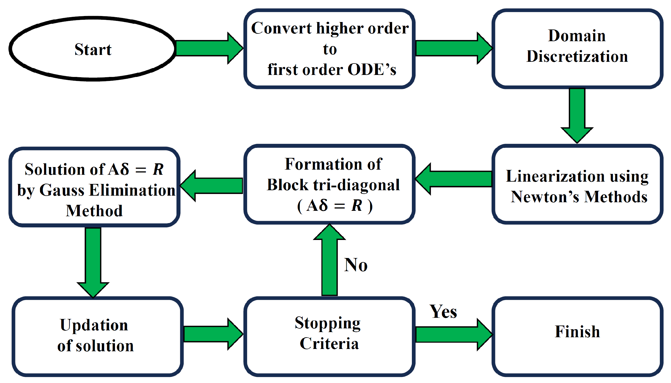
3. Computational Solution

The Keller Box technique is a highly effective finite difference method employed to solve parabolic problems, particularly those that contain systems of nonlinear coupled ordinary differential equations (ODEs). By following the procedures, the higher-order nonlinear problem can be resolved.

• In the beginning, the nonlinear coupled ordinary differential equation system (8)–(12) is converted into a system of coupled first-order ODEs.
• Next, these equations are discretized utilizing an appropriate finite difference scheme.
• Newton’s method is utilized throughout the discretization procedure to achieve equation linearization.
• The block tri-diagonal matrices are then constructed utilizing the system of linear equations.
• Finally, the tri-diagonal matrices are solved using the Gauss elimination method [28,38].

The choice of initial guesses gives the problem a better convergence and minimum error. Here, the following initial guesses are taken:

$$\begin{array}{c}\hfill \frac{d{f}_0}{d\xi }=1-e^{-\xi },{\theta }_0=e^{-\xi },{\phi }_0=e^{-\xi },{\chi }_0=e^{-\xi }.\end{array}$$

The step size $h_j=0.005$ appears to provide acceptable accuracy in this method, and we adhered to the 10⁻⁶ error tolerance in all cases to obtain a better result. The values presented in

Table 1. Validation with previous results and keeping $R_b=P_e=N_1=M=0$, $\mathsf{\Gamma }=E_1=K_0=L_b=Q_0=E_c=0$.

	Lin [2]		Current Work
${\mathit{P}}_{\mathit{r}}$	${\mathit{C}}_{\mathit{f}}$	$-\frac{\mathit{d}\mathit{\theta }}{\mathit{d}\mathit{\xi }}\left(\mathbf{0}\right)$	${\mathit{C}}_{\mathit{f}}$	$-\frac{\mathit{d}\mathit{\theta }}{\mathit{d}\mathit{\xi }}\left(\mathbf{0}\right)$
0.72	0.898300	1.523690	0.937134	1.570613
1	0.784465	1.391746	0.832299	1.439581
2	0.652528	1.162097	0.700363	1.209932
4	0.463073	0.980958	0.510909	1.028794
6	0.396883	0.891957	0.444721	0.939794
8	0.355639	0.834979	0.403477	0.882817
10	0.326555	0.793885	0.374394	0.841724
100	0.133715	0.483722	0.181555	0.531562

for each parameter adjustment exhibit a high degree of concordance, indicating that the validation of the methodology has been effectively executed. The outcomes validate our Keller Box approach based on finite differences. Figure 2 shows the flowchart for the Keller Box method for better understanding.

4. Result and Findings

This model graphically depicts a bioconvective fluid flow’s heat and mass transfer. All of the parameter values in this model were chosen in the ways shown below. $S_c=2$, $N_r=0.5$, $L_b=0.5$, $P_e=0.3$, $\sigma =0.4$, $R_b=0.5$, $K_r=0.4$, $E_1=1$, $K=0.4$, $N_1=2$, $\mathsf{\Gamma }=1$, $M=1$, $E_c=0.3$, $Q_0=-0.1$, $P_r=6.8$. All the values remain the same unless explicitly stated. In all of the figures, the first part of the graph represents the vertical cone (where $\omega \ne 0$), and the second part of the graph represents the vertical plate (where $\omega =0$).

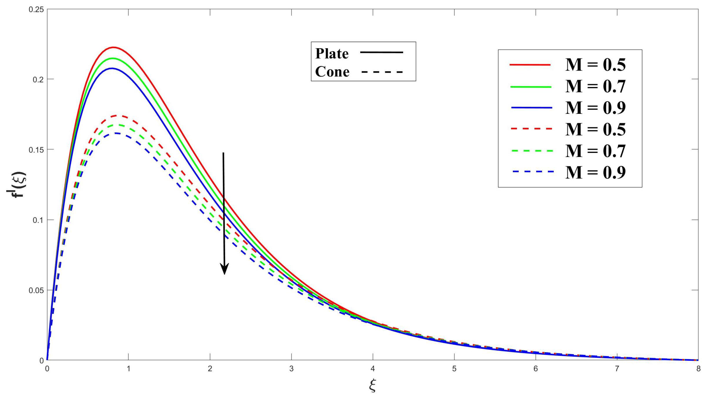
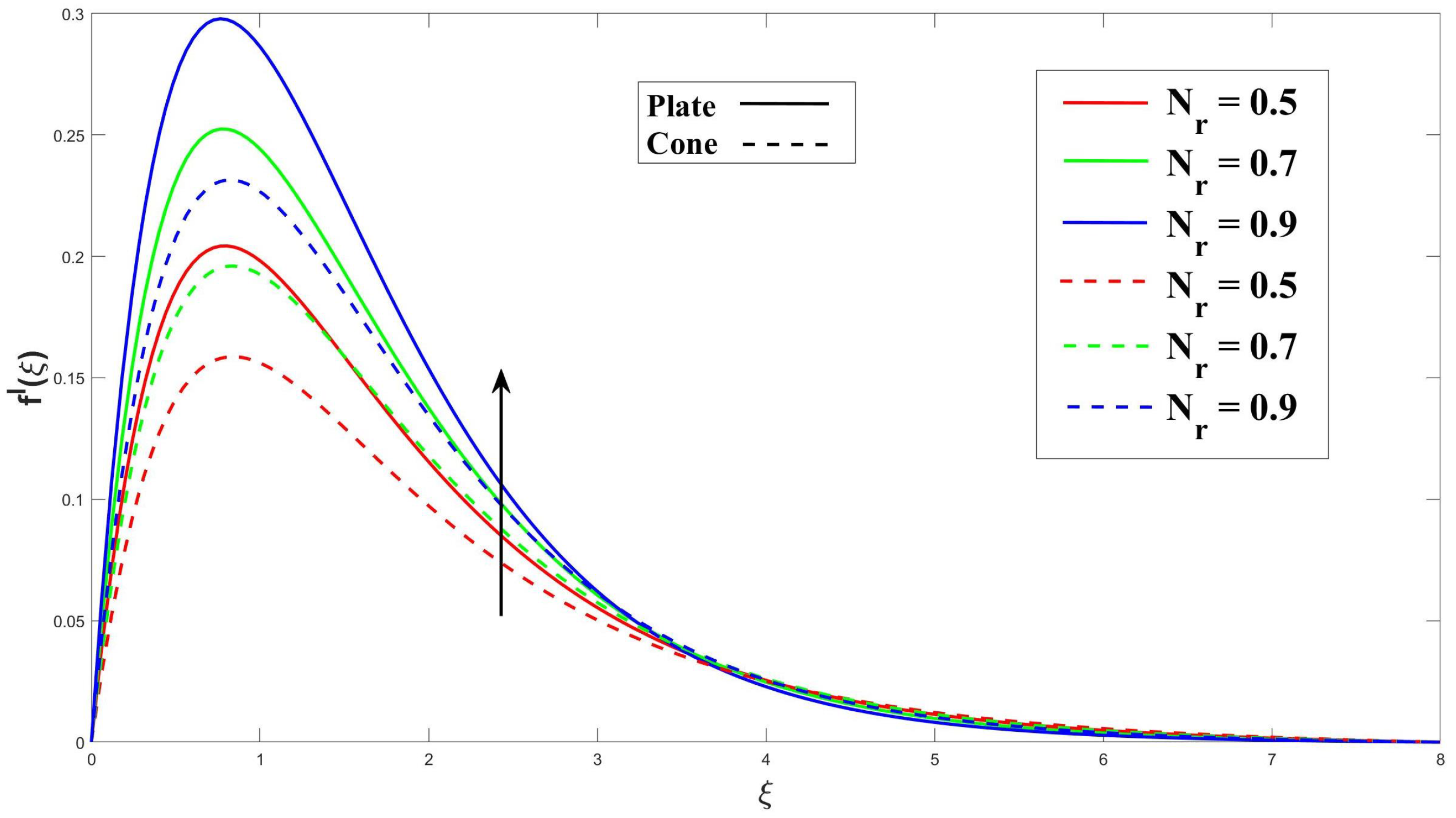
4.1. Velocity Profile

The data presented in Figure 3 illustrate a clear relationship between the Eyring–Powell fluid parameter (K) and the velocity profile. Specifically, as the value of K increases, there is a noticeable decrease in the velocity profile. As a result of the effect of the frictional drag force, this drop is more pronounced on a horizontal surface in a cone. The cone has a stronger impact on the fluid flow velocity than the upright plate. Figure 4 clearly demonstrates that an increase in the magnetohydrodynamic (MHD) parameter leads to a significant reduction in the velocity profile for both the cone and plate surfaces. As a result of Lorentz’s force, related to the fluid flow paths, being perpendicular to the fluid flow path, it contributes to this reduction. Therefore, the plate and cone have an increase in the thickness of the velocity boundary layer. Figure 5 illustrates that a higher porosity parameter ($\mathsf{\Gamma }$) leads to a thicker momentum boundary layer. The porosity of the cone or plate surface modifies the drag force exerted on it. Surfaces with higher porosity allow fluid to pass through, thereby reducing the drag compared to surfaces that divert the fluid around them. Furthermore, Figure 6 and Figure 7 illustrate that an increase in the buoyancy parameter ($N_r$) and the Rayleigh number ($R_b$) lead to a noticeable amplification of the velocity profiles for both the plate and cone surfaces. The buoyancy ratio factor represents a fluid flow’s buoyancy-to-viscous-force ratio. The fluid’s efficiency to transfer momentum is improved by increasing this parameter, which raises the velocity profile.

It is noticeable from

Table 2. The local Nusselt number ($-{\theta }^{\prime }\left(0\right)$) and skin friction ($C_f$).

								${\mathit{C}}_{\mathit{f}}$		$-\frac{\mathit{d}\mathit{\theta }}{\mathit{d}\mathit{\xi }}\left(0\right)$
$\mathit{K}$	$\mathit{M}$	$\mathsf{\Gamma }$	${\mathit{E}}_{\mathit{c}}$	${\mathit{Q}}_{\mathbf{0}}$	${\mathit{N}}_{\mathit{r}}$	${\mathit{R}}_{\mathit{b}}$	${\mathit{P}}_{\mathit{r}}$	$\mathit{\omega }=\mathbf{0}$	$\mathit{\omega }\ne \mathbf{0}$	$\mathit{\omega }=\mathbf{0}$	$\mathit{\omega }\ne \mathbf{0}$
0.3	1	1	0.3	-0.1	0.5	0.5	6.8	0.8276611	0.6264303	0.7739583	0.7403775
0.5								0.8470072	0.6437625	0.7457247	0.7115269
0.7								0.8696108	0.6609366	0.7206157	0.6863384
	0.5							0.8470072	0.6437628	0.7457247	0.7115263
	0.7							0.8696108	0.6609369	0.7206157	0.6863379
	0.9							0.8925743	0.6771554	0.6982958	0.6641069
		0.3						0.8968186	0.6879259	0.7850504	0.7688138
		0.5						0.8749441	0.6681376	0.7827928	0.7607958
		0.7						0.8548882	0.6502805	0.7796985	0.7526417
			0.3					0.8256691	0.6241277	0.7720337	0.7373497
			0.6					0.833363	0.6280245	0.5775666	0.6255623
			0.9					0.8413745	0.6320319	0.3736041	0.5103081
				−0.1				0.7913353	0.5908076	1.0579258	1.0455024
				0				0.810632	0.6096124	0.7892907	0.7541461
				0.1				0.8346166	0.6345497	0.4739704	0.3980173
					0.5			0.8127954	0.6117887	0.7601186	0.7219011
					1			0.9791096	0.7483265	0.7676565	0.7561591
					1.5			1.1181125	0.8755358	0.7502905	0.7703388
						0.5		0.8127954	0.6117887	0.7601186	0.7219011
						1		0.9772917	0.7473042	0.7676901	0.7558917
						1.5		1.114516	0.8730627	0.7512737	0.7700876
							6.8	0.8127954	0.6117887	0.7601186	0.7219011
							7.8	0.8052942	0.6057737	0.7906545	0.7544055
							8.8	0.7987378	0.6004823	0.8176548	0.7837094

that raising the Eyring–Powell fluid parameter (K), the MHD (M) factor, and the permeability parameter ($\mathsf{\Gamma }$), the skin friction ($C_f$) number over the cone and plate surfaces increases. The local skin friction ($C_f$) is further increased by raising the Rayleigh parameter ($R_b$) and the buoyancy parameter ($N_r$).

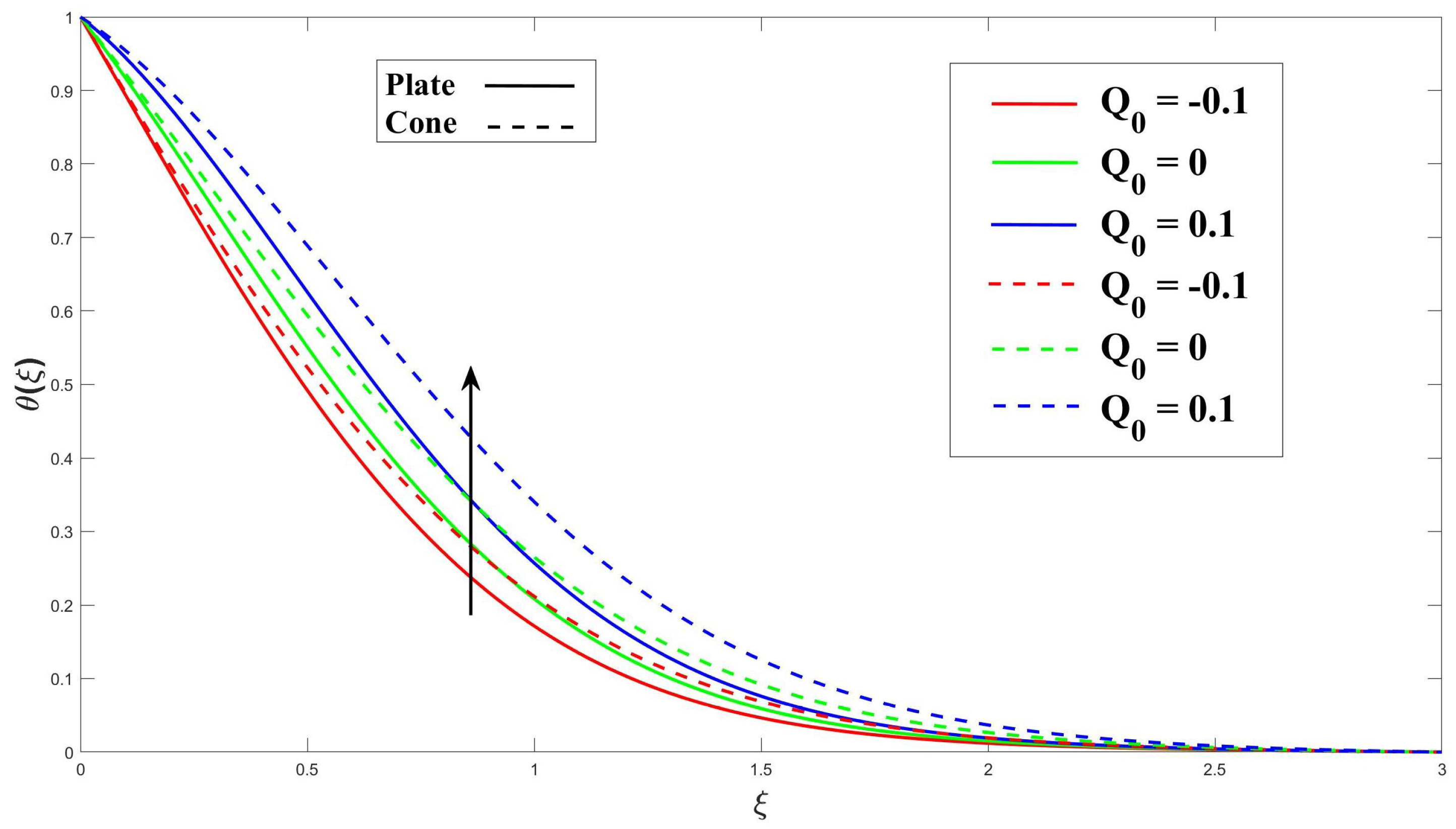
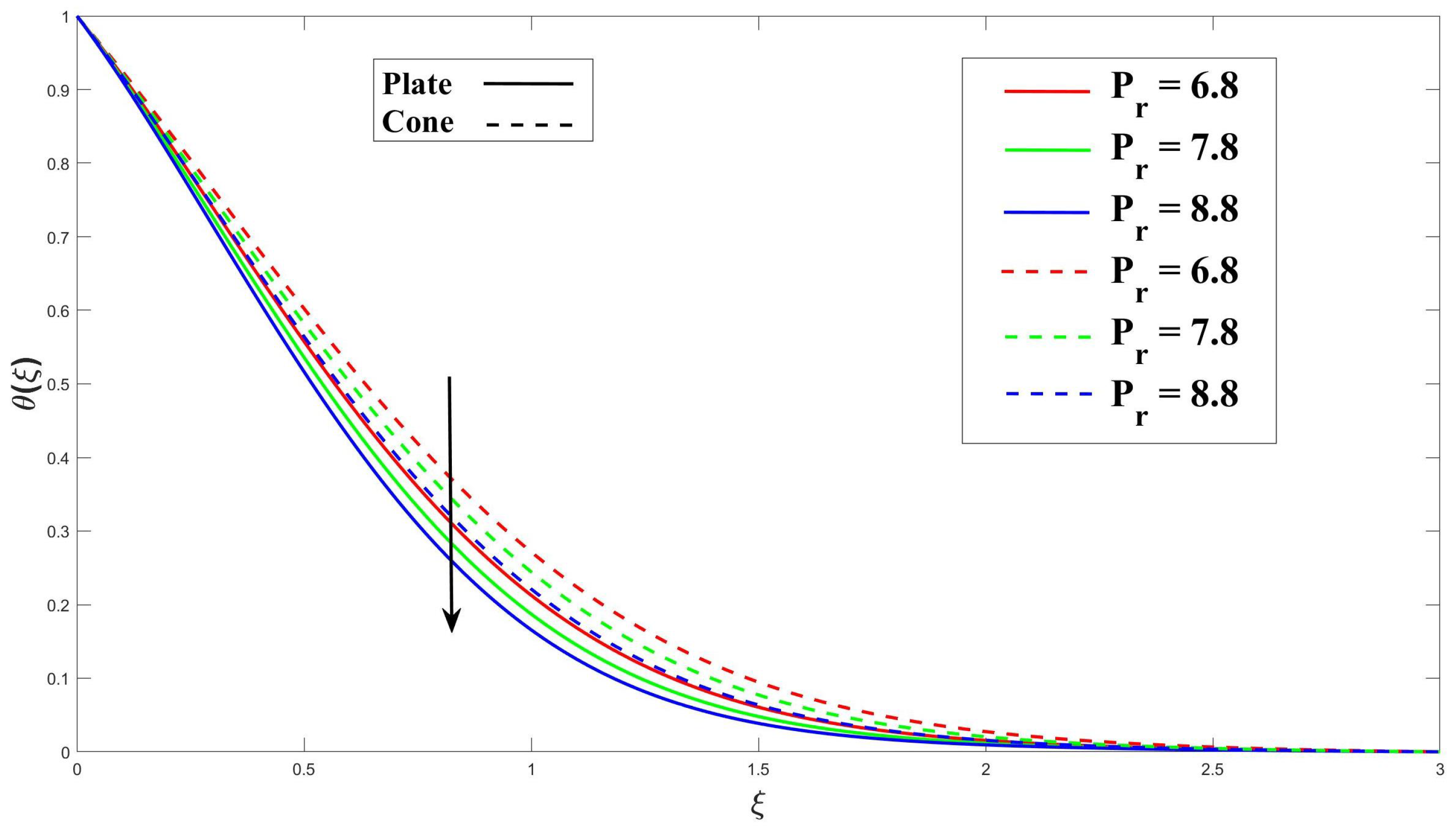
4.2. Temperature Profile

Figure 8 highlights the significance of the Eyring–Powell fluid parameter (K) in the model, demonstrating that increasing this parameter enhances heat transfer. Additionally, the cone surface exhibits a smaller thermal boundary layer (TBL) thickness compared to the vertical plate, leading to a higher heat transfer rate. Figure 9 shows explicitly how increasing the MHD (M) factor enhances heat transfer. The interactions between the magnetic field and the moving charged particles in the electrically conducting fluid are responsible for this improvement. The resulting Lorentz force affects the fluid’s velocity and direction, ultimately enhancing heat transfer. In Figure 10, the primary impact of the porosity ($\mathsf{\Gamma }$) on heat transfer is the increased surface area available for heat exchange. The solid matrix of the porous medium provides a larger surface area for the fluid to come into contact with, promoting higher heat transfer rates. This characteristic is particularly advantageous in applications requiring efficient heat transfer, such as heat exchangers or catalytic reactors. Figure 11 shows that as the Eckert number ($E_c$) increases, the viscous dissipation within the fluid becomes more pronounced. This dissipation converts some of the fluid’s kinetic energy into thermal energy, resulting in increased heating within the boundary layer. Consequently, more heat is dissipated near the cone and plate surfaces, leading to a decrease in the thickness of the thermal boundary layer (TBL). In Figure 12, the presence of a uniform heat source or sink affects the temperature distribution near the boundary surface. A higher heat source/sink parameter ($Q_0$) indicates a stronger heat generation or absorption within the non-Newtonian fluid, and causes a stronger temperature gradient near the boundary and a thicker thermal boundary layer (TBL). The Prandtl number ($P_r$) and its depiction of the relationship between thermal and momentum diffusivity in the fluid flow are shown in Figure 13. The TBL thickness contributes to its large value as the $P_r$ grows.

Superior heat transfer performance of the cone surface compared to the plate surface can be attributed to the differences in fluid flow behavior. When a fluid flows over a flat plate, it tends to slow down and accumulate near the surface, resulting in a thicker thermal boundary layer and a lower rate of heat transfer. On the other hand, when a fluid flows over a curved surface, like a cone, it is forced to speed up and conform to the surface’s curvature. This leads to a thinner thermal boundary layer and a higher rate of heat transfer.

Referring to Table 2, as we increase the Eyring–Powell fluid parameter (K), Eckert number ($E_c$), heat source/sink parameter ($Q_0$), MHD (M) parameter, or the porosity ($\mathsf{\Gamma }$) parameter, $-{\theta }^{\prime }\left(0\right)$ decreases for both the surfaces. Also, a higher Prandtl ($P_r$) number leads to a higher $-{\theta }^{\prime }\left(0\right)$.

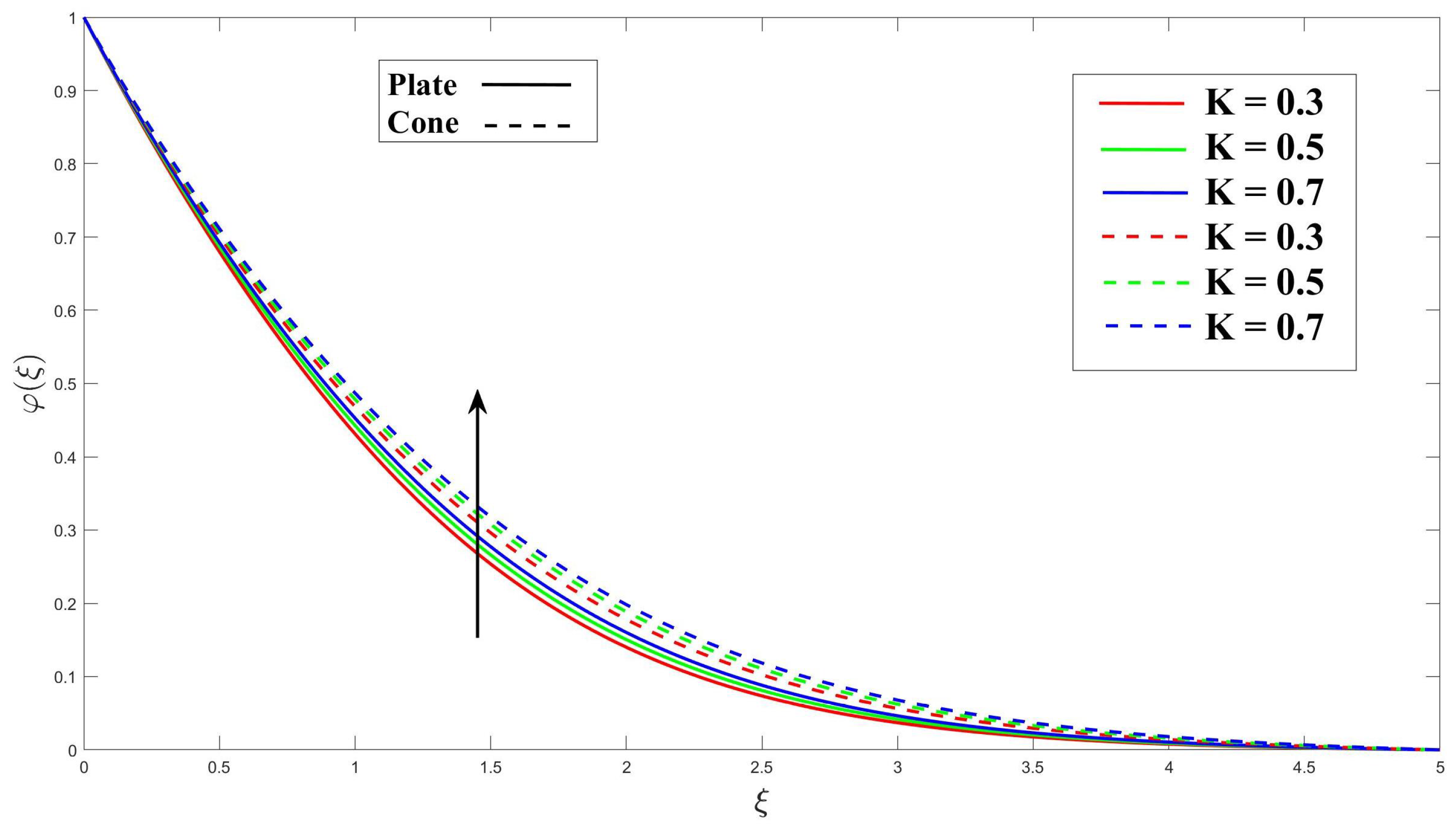
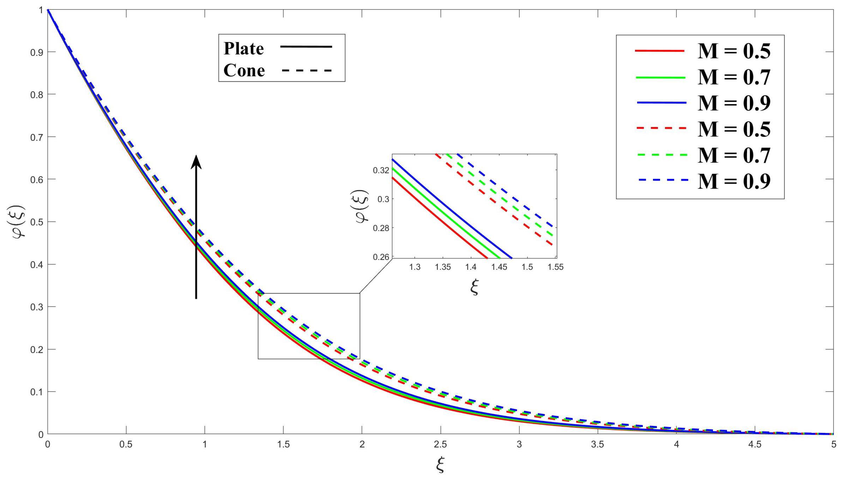
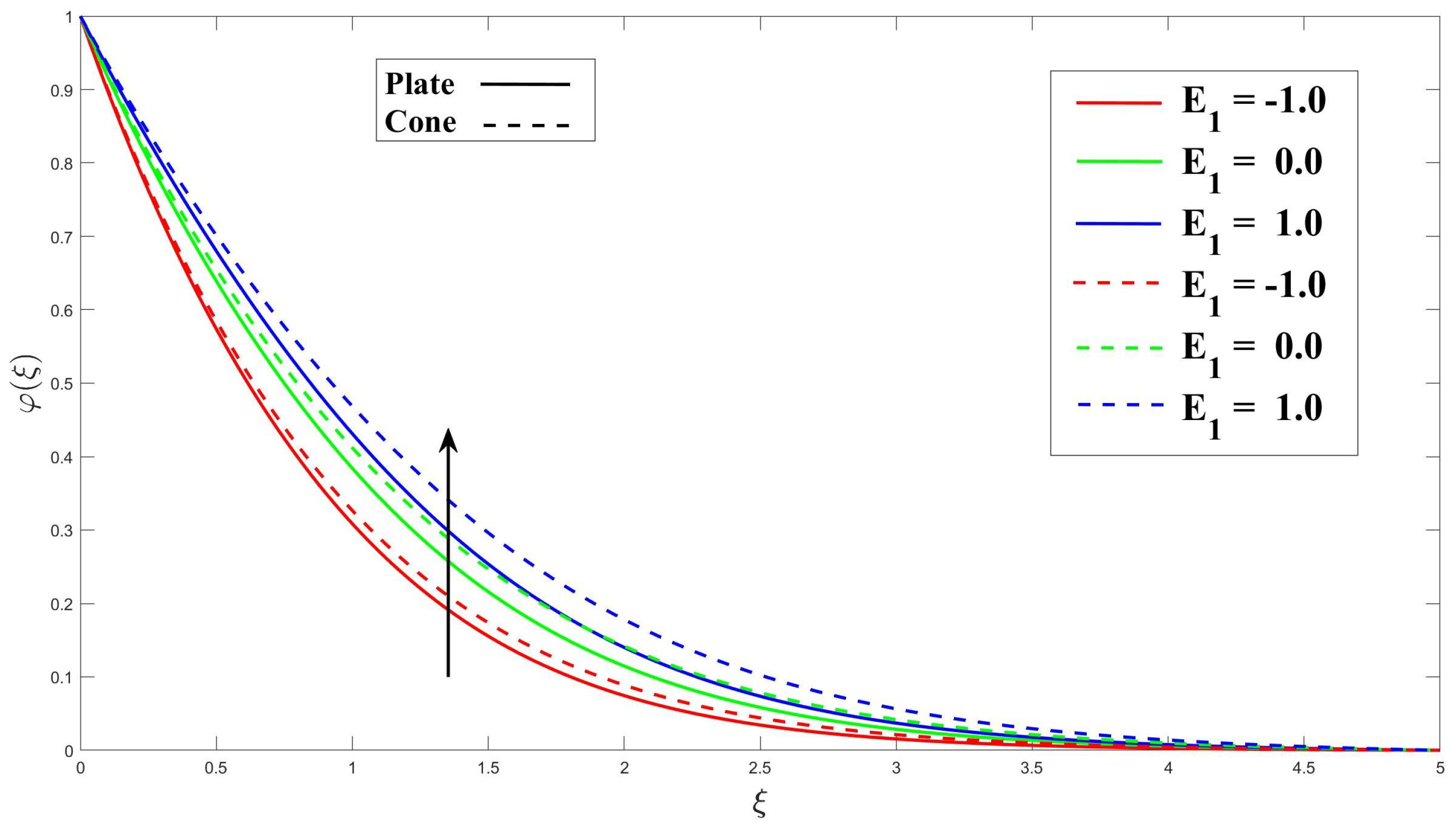
4.3. Concentration Profile

In Figure 14, increase in the Eyring–Powell fluid parameter (K) results in an increased rate of concentration diffusion. This effect can be attributed to the increase in the stress tensor, which enhances fluid mixing and dispersion. As a result, the concentration profiles are affected. Moving on to Figure 15, the application of magnetohydrodynamics (MHD) and an increase in the MHD parameter (M) are shown to influence the thickness of the concentration boundary layer (CBL). Applying MHD has the potential to improve fluid mixing, thereby enhancing the mass transfer process. Figure 16 explains the impact of porosity and increasing the porosity parameter ($\mathsf{\Gamma }$) on the thickness of the concentration boundary layer (CBL). The porosity parameter ($\mathsf{\Gamma }$) can enhance fluid mixing, leading to an improved mass transfer process. In Figure 17, increasing the chemical reaction parameter ($K_0$) in the fluid flow results in more significant chemical reactions. Consequently, the concentration boundary layer (CBL) thickness increases to accommodate the changing concentration distribution near the boundary surface. The activation energy is the minimum energy required for a chemical reaction to occur. Figure 18 shows that as the activation energy parameter ($E_1$) increases, the barrier for the reaction becomes more significant. As a result, fewer reactive species possess enough energy to overcome this barrier and participate in the reaction. As a result of these changes, the observed effect is a decrease in the reaction rate and the formation of a thinner CBL. Figure 19 illustrates that the CBL thickness obtains its higher level as the Schmidt number ($S_c$) rises.

Upon looking at Figure 14, Figure 15, Figure 16, Figure 17, Figure 18 and Figure 19, we can observe that the cone and plate surfaces have different shapes. The cone’s shape changes along its surface, while the plate’s surface stays the same. This difference in shape affects how the fluid moves over them and leads to variations in how the substance is distributed. Specifically, the fluid near the cone’s surface has a higher concentration than near the plate’s surface. This happens because the particles close to the cone’s surface have a shorter distance to cover the same area compared to particles near the plate’s surface. As a result, there are faster flows and more noticeable differences in concentration near the cone’s surface. Additionally, the curved shape of the cone delays the separation of the flow from the surface compared to the flat plate. This delay contributes to the higher concentration gradient near the cone’s surface.

The convincing evidence in

Table 3. The local density of microorganisms ($-{\chi }^{\prime }\left(0\right)$) and local Sherwood number ($-{\phi }^{\prime }\left(0\right)$).

								$-\frac{\mathit{d}\mathit{\phi }}{\mathit{d}\mathit{\xi }}\left(0\right)$		$-\frac{\mathit{d}\mathit{\chi }}{\mathit{d}\mathit{\xi }}\left(0\right)$
$\mathit{K}$	$\mathit{M}$	$\mathsf{\Gamma }$	${\mathit{K}}_{\mathbf{0}}$	${\mathit{E}}_{\mathbf{1}}$	${\mathit{S}}_{\mathit{c}}$	${\mathit{L}}_{\mathit{b}}$	${\mathit{P}}_{\mathit{e}}$	$\mathit{\omega }=\mathbf{0}$	$\mathit{\omega }\ne \mathbf{0}$	$\mathit{\omega }=\mathbf{0}$	$\mathit{\omega }\ne \mathbf{0}$
0.3	1	1	0.3	1	1	0.5	0.7	0.6067597	0.5806644	0.6308123	0.5936918
0.5								0.5990076	0.5748254	0.6196365	0.5848375
0.7								0.5924407	0.5699847	0.6100861	0.5773683
	0.5							0.5990076	0.5748254	0.6196365	0.5848376
	0.7							0.5924407	0.5699848	0.6100861	0.5773683
	0.9							0.5868241	0.5659283	0.6018375	0.5709893
		0.3						0.6295077	0.5997143	0.6612226	0.6200352
		0.5						0.6220819	0.5933534	0.6513683	0.6113485
		0.7						0.6154555	0.5877915	0.6425197	0.6036701
			0.3					0.6067597	0.5806644	0.6308123	0.5936919
			0.5					0.725906	0.7091557	0.7572944	0.7271007
			0.7					0.8360051	0.8261611	0.8846352	0.8600359
				−1				1.0086156	0.9978203	1.0697198	1.0428716
				0				0.7667685	0.7507371	0.7902278	0.7599957
				1				0.6067597	0.5806644	0.6308123	0.5936919
					0.5			0.5332354	0.5212129	0.5921514	0.5620565
					1			0.6067597	0.5806644	0.6308123	0.5936919
					1.5			0.6676092	0.6315215	0.6684937	0.6246851
						0.3		0.4992610	0.494676	0.5771215	0.5497044
						0.5		0.5332354	0.5212129	0.5921514	0.5620565
						0.7		0.5644747	0.5461578	0.6075921	0.5746854
							0.5	0.6106761	0.5836606	0.536743	0.5002762
							0.7	0.6067597	0.5806644	0.6308123	0.5936919
							0.9	0.6030955	0.5778879	0.7215598	0.6838918

shows that $-{\phi }^{\prime }\left(0\right)$ decreases for both the surfaces as the Eyring–Powell (non-Newtonian) fluid (K) parameter, the magnetohydrodynamics parameter (M), the activation energy parameter ($E_1$), and the porosity parameter ($\mathsf{\Gamma }$) increase. On the other hand, with a rise in the Schmidt number ($S_c$) and the chemical reaction parameter ($K_0$), the $-{\phi }^{\prime }\left(0\right)$ value increases.

4.4. Microorganism Profile

Figure 20 and Figure 21 demonstrate the effects of applying magnetohydrodynamics (M) and porosity ($\mathsf{\Gamma }$) on fluid flow containing microorganisms. These effects enhance the diffusion rate of microorganisms and reduce the minimum boundary layer thickness for their diffusion. The interaction of the magnetic field and the flowing fluid results in the magnetohydrodynamics (M) effect. This interaction leads to the induction of electrical currents, which, in turn, promotes mixing and diffusion of microorganisms. The presence of a porous medium creates a convoluted path for fluid flow, promoting mixing and transport of microorganisms within the fluid. In Figure 22 and Figure 23, it is shown that increasing the chemical reaction parameter ($K_0$) leads to a decrease in the microorganisms’ boundary layer thickness due to more significant chemical reactions. On the other hand, increasing the activation energy parameter ($E_1$) results in a thinner boundary layer as it hinders the reaction rate within the microorganisms. Moving on to Figure 24, it is explained that in fluid flow with swimming microorganisms, rises in the Péclet number ($P_e$) enhance fluid mixing due to the motion of the microorganisms. This enhanced mixing promotes nutrient uptake, overall growth of the microorganisms, and changes in their spatial distribution within the fluid. The bioconvection’s stability and pattern creation are clearly impacted by an increase in the Lewis number ($L_b$), as seen in Figure 25. The buoyant forces that propel bioconvection are impacted by this change in the equilibrium of diffusion mechanisms, which reduces the stability of the biological convection patterns.

In Table 3, the local microorganism density number ($-{\chi }^{\prime }\left(0\right)$) exhibits distinct behavior based on the variations in the different parameters. Firstly, when the Eyring–Powell fluid parameter (K), the activation energy parameter ($E_1$), the magnetohydrodynamics (M) parameter, and the porosity parameter ($\mathsf{\Gamma }$) are increased for both the surfaces, the local microorganism density number ($-{\chi }^{\prime }\left(0\right)$) decreases. This suggests that these parameters hinder the growth or proliferation of microorganisms, resulting in a lower density within the boundary layer. On the other hand, an increase in the local microbe density number ($-{\chi }^{\prime }\left(0\right)$) is caused by a decrease in the nonlinear chemical reaction parameter ($K_0$), Péclet number ($P_e$), and Lewis number ($L_b$). These parameters, which are associated with chemical reactions and bioconvection processes, enhance the growth or transport of microorganisms, resulting in a higher density within the boundary layer.

5. Conclusions

The current study employed a non-Newtonian (Eyring–Powell) fluid simulation to analyse the heat and mass transfer characteristics of a bioconvective fluid. Understanding the flow over a permeable cone and plate was the primary objective. In order to gain a comprehensive understanding of the mechanisms underlying mass and heat transfer, we conducted an investigation into the impact of several parameters: magnetohydrodynamics (MHD), porosity, viscous dissipation, uniform heat source/sink, chemical reaction, and activation energy. The nonlinear partial differential equations (PDEs) are converted to ordinary differential equations (ODEs) via a similarity transformation (ST). Utilizing the Keller Box (KB) finite difference method, these equations are solved. By applying this methodology, we obtained outcomes that validated our findings established in previous studies.

• While increasing the MHD $\left(M\right)$ and porosity $\left(\mathsf{\Gamma }\right)$ parameter:
  • Heat transfer increased by 14.24% and 19.36%;
  • Mass transfer increased by 13.20% and 16.4%;
  • Microorganism diffusion increased by 14.67% and 15.37%.
• While increasing the Eyring–Powell fluid $\left(K\right)$ parameter:
  • Heat transfer increased by 8.47%;
  • Mass transfer increased by 8.45%.
• While increasing the Eckert number $\left(E_c\right)$ and heat source/sink $\left(Q_0\right)$ parameter:
  • Heat transfer increased by 6.32% and 15.34%.
• While decreasing the chemical reaction $\left(K_0\right)$ parameter:
  • Mass transfer increased by 16.6%;
  • Microorganism diffusion increased by 3.3%.
• While increasing the activation energy $\left(E_1\right)$ parameter:
  • Mass transfer increased by 18.2%;
  • Microorganism diffusion increased by 4.1%.

In the future, researchers may undertake further comprehensive examinations of the mass and heat transfer dynamics of Eyring–Powell (non-Newtonian) fluids that contain microorganisms in situations where conditions are unsteady.

References

1. Hansen, A.; Na, T. Similarity solutions of laminar, incompressible boundary layer equations of non-Newtonian fluids. J. Basic Eng. 1968, 90, 71–74. [Google Scholar] [CrossRef]
2. Lin, F. Laminar free convection from a vertical cone with uniform surface heat flux. Lett. Heat Mass Transf. 1976, 3, 49–58. [Google Scholar]
3. Shima, A.; Tsujino, T. The effect of polymer concentration on the bubble behaviour and impulse pressure. Chem. Eng. Sci. 1981, 36, 931–935. [Google Scholar] [CrossRef]
4. Hartnett, J.P.; Kwack, E. Prediction of friction and heat transfer for viscoelastic fluids in turbulent pipe flow. Int. J. Thermophys. 1986, 7, 53–63. [Google Scholar] [CrossRef]
5. Sirohi, V.; Timol, M.; Kalthia, N. Powell-Eyring model flow near an accelerated plate. Fluid Dyn. Res. 1987, 2, 193. [Google Scholar] [CrossRef]
6. Kumari, M.; Pop, I.; Nath, G. Mixed convection along a vertical cone. Int. Commun. Heat Mass Transf. 1989, 16, 247–255. [Google Scholar] [CrossRef]
7. Abd-el Hafiz, A.M. Steady flow in an infinite cylindrical pipe of a mixture consisting of a newtonian and a non-Newtonian phase (the case of eyring Powell model). J. Phys. Soc. Jpn. 1991, 60, 879–883. [Google Scholar] [CrossRef]
8. Kafoussias, N. MHD free convective flow through a non homogeneous porous medium over an isothermal cone surface. Mech. Res. Commun. 1992, 19, 89–99. [Google Scholar] [CrossRef]
9. Hossain, M.; Paul, S. Free convection from a vertical permeable circular cone with non-uniform surface temperature. Acta Mech. 2001, 151, 103–114. [Google Scholar] [CrossRef]
10. Eldabe, N.; Hassan, A.; Mohamed, M.A. Effect of couple stresses on the MHD of a non-Newtonian unsteady flow between two parallel porous plates. Z. Naturforschung A 2003, 58, 204–210. [Google Scholar] [CrossRef]
11. Yürüsoy, M. A Study of pressure distribution of a slider bearing lubricated with Powell-Eyring fluid. Turk. J. Eng. Environ. Sci. 2003, 27, 299–304. [Google Scholar]
12. Barth, W.L.; Carey, G.F. On a natural-convection benchmark problem in non-Newtonian fluids. Numer. Heat Transf. Part Fundam. 2006, 50, 193–216. [Google Scholar] [CrossRef]
13. Pullepu, B.; Ekambavanan, E.; Chamkha, A. Unsteady laminar natural convection from a non-isothermal vertical cone. Nonlinear Anal. Model. Control 2007, 12, 525–540. [Google Scholar] [CrossRef]
14. Pullepu, B.; Ekambavanan, K.; Chamkha, A. Unsteady laminar free convection from a vertical cone with uniform surface heat flux. Nonlinear Anal. Model. Control 2008, 13, 47–60. [Google Scholar] [CrossRef]
15. Patel, M.; Timol, M. Numerical treatment of Powell–Eyring fluid flow using method of satisfaction of asymptotic boundary conditions (MSABC). Appl. Numer. Math. 2009, 59, 2584–2592. [Google Scholar] [CrossRef]
16. Patel, M.; Timol, M. The stress-strain relationship for visco-inelastic non-Newtonian fluids. Int. J. Appl. Math. Mech. 2010, 6, 79–93. [Google Scholar]
17. Raju, C.; Jayachandrababu, M.; Sandeep, N.; Mohankrishna, P. Influence of non-uniform heat source/sink on MHD nanofluid flow over a moving vertical plate in porous medium. Int. J. Sci. Eng. Res 2015, 6, 31–42. [Google Scholar]
18. Jayachandra Babu, M.; Sandeep, N.; Raju, C.S. Heat and mass transfer in MHD Eyring-Powell nanofluid flow due to cone in porous medium. Int. J. Eng. Res. Afr. 2016, 19, 57–74. [Google Scholar] [CrossRef]
19. Koriko, O.; Animasaun, I.; Reddy, M.G.; Sandeep, N. Scrutinization of thermal stratification, nonlinear thermal radiation and quartic autocatalytic chemical reaction effects on the flow of three-dimensional Eyring-Powell alumina-water nanofluid. Multidiscip. Model. Mater. Struct. 2018, 14, 261–283. [Google Scholar] [CrossRef]
20. Khan, M.; Irfan, M.; Khan, W.; Ahmad, L. Modeling and simulation for 3D magneto Eyring–Powell nanomaterial subject to nonlinear thermal radiation and convective heating. Results Phys. 2017, 7, 1899–1906. [Google Scholar] [CrossRef]
21. Khan, I.; Khan, M.; Malik, M.Y.; Salahuddin, T. Mixed convection flow of Eyring-Powell nanofluid over a cone and plate with chemical reactive species. Results Phys. 2017, 7, 3716–3722. [Google Scholar] [CrossRef]
22. Rehman, K.U.; Saba, N.U.; Malik, M.; Malik, A.A. Encountering heat and mass transfer mechanisms simultaneously in Powell-Erying fluid through Lie symmetry approach. Case Stud. Therm. Eng. 2017, 10, 541–549. [Google Scholar] [CrossRef]
23. Simon, S.G.; Bira, B.; Zeidan, D. Optimal systems, series solutions and conservation laws for a time fractional cancer tumor model. Chaos Solitons Fractals 2023, 169, 113311. [Google Scholar] [CrossRef]
24. Waqas, M.; Khan, M.I.; Hayat, T.; Alsaedi, A.; Khan, M.I. On Cattaneo–Christov double diffusion impact for temperature-dependent conductivity of Powell–Eyring liquid. Chin. J. Phys. 2017, 55, 729–737. [Google Scholar] [CrossRef]
25. Balazadeh, N.; Sheikholeslami, M.; Ganji, D.D.; Li, Z. Semi analytical analysis for transient Eyring-Powell squeezing flow in a stretching channel due to magnetic field using DTM. J. Mol. Liq. 2018, 260, 30–36. [Google Scholar] [CrossRef]
26. Layek, G.; Mandal, B.; Bhattacharyya, K. Dufour and soret effects on unsteady heat and mass transfer for powell-eyring fluid flow over an expanding permeable sheet. J. Appl. Comput. Mech. 2020, 6, 985–998. [Google Scholar]
27. Khan, S.U.; Waqas, H.; Muhammad, T.; Imran, M.; Aly, S. Simultaneous effects of bioconvection and velocity slip in three-dimensional flow of Eyring-Powell nanofluid with Arrhenius activation energy and binary chemical reaction. Int. Commun. Heat Mass Transf. 2020, 117, 104738. [Google Scholar] [CrossRef]
28. Khan, B.M.H.; Gaffar, S.A.; Beg, O.A.; Kadir, A.; Reddy, P.R. Computation of Eyring-Powell micropolar convective boundary layer flow from an inverted non-isothermal cone: Thermal polymer coating simulation. Comput. Therm. Sci. Int. J. 2020, 12, 329–344. [Google Scholar] [CrossRef]
29. Khan, N.M.; Bacha, H.B.; Pan, K.; Saeed, T. Nonlinear Eyring–Powell bioconvective nanofluid flow over a vertical plate with temperature dependent viscosity and surface suction. Int. Commun. Heat Mass Transf. 2021, 128, 105602. [Google Scholar] [CrossRef]
30. Oke, A. Coriolis effects on MHD flow of MEP fluid over a non-uniform surface in the presence of thermal radiation. Int. Commun. Heat Mass Transf. 2021, 129, 105695. [Google Scholar] [CrossRef]
31. Qaiser, D.; Zheng, Z.; Khan, M.R. Numerical assessment of mixed convection flow of Walters-B nanofluid over a stretching surface with Newtonian heating and mass transfer. Therm. Sci. Eng. Prog. 2021, 22, 100801. [Google Scholar] [CrossRef]
32. Xia, W.F.; Haq, F.; Saleem, M.; Khan, M.I.; Khan, S.U.; Chu, Y.M. Irreversibility analysis in natural bio-convective flow of Eyring-Powell nanofluid subject to activation energy and gyrotactic microorganisms. Ain Shams Eng. J. 2021, 12, 4063–4074. [Google Scholar] [CrossRef]
33. Fatunmbi, E.O.; Adeosun, A.T.; Salawu, S.O. Irreversibility Analysis for Eyring–Powell Nanoliquid Flow Past Magnetized Riga Device with Nonlinear Thermal Radiation. Fluids 2021, 6, 416. [Google Scholar] [CrossRef]
34. Habib, U.; Abdal, S.; Siddique, I.; Ali, R. A comparative study on micropolar, Williamson, Maxwell nanofluids flow due to a stretching surface in the presence of bioconvection, double diffusion and activation energy. Int. Commun. Heat Mass Transf. 2021, 127, 105551. [Google Scholar] [CrossRef]
35. Baranovskii, E.S. Optimal boundary control of the Boussinesq approximation for polymeric fluids. J. Optim. Theory Appl. 2021, 189, 623–645. [Google Scholar] [CrossRef]
36. Farooq, M.; Anjum, A.; Rehman, S.; Malik, M. Entropy analysis in thermally stratified Powell-Eyring magnesium-blood nanofluid convection past a stretching surface. Int. Commun. Heat Mass Transf. 2022, 138, 106375. [Google Scholar] [CrossRef]
37. El-Dabe, N.; Mostapha, D.R. Hall current effects on electro-magneto-dynamic peristaltic flow of an Eyring–Powell fluid with mild stenosis through a uniform and non-uniform annulus. Indian J. Phys. 2022, 96, 2841–2853. [Google Scholar] [CrossRef]
38. Thameem Basha, H.; Reddy, S.; Prasad, V.R.; Son, K.J.; Ahammad, N.A.; Akkurt, N. Non-similar solutions and sensitivity analysis of nano-magnetic Eyring–Powell fluid flow over a circular cylinder with nonlinear convection. Waves Random Complex Media 2022. [Google Scholar] [CrossRef]
39. Khan, S.U.; Irfan, M.; Khan, M.I.; Abbasi, A.; Rahman, S.U.; Niazi, U.M.; Farooq, S. Bio-convective Darcy-Forchheimer oscillating thermal flow of Eyring-Powell nanofluid subject to exponential heat source/sink and modified Cattaneo–Christov model applications. J. Indian Chem. Soc. 2022, 99, 100399. [Google Scholar] [CrossRef]
40. Anjum, N.; Khan, W.; Hobiny, A.; Azam, M.; Waqas, M.; Irfan, M. Numerical analysis for thermal performance of modified Eyring Powell nanofluid flow subject to activation energy and bioconvection dynamic. Case Stud. Therm. Eng. 2022, 39, 102427. [Google Scholar] [CrossRef]
41. Bhattacharyya, A.; Kumar, R.; Bahadur, S.; Seth, G. Modeling and interpretation of peristaltic transport of Eyring–Powell fluid through uniform/non-uniform channel with Joule heating and wall flexibility. Chin. J. Phys. 2022, 80, 167–182. [Google Scholar] [CrossRef]
42. Pasha, A.A.; Islam, N.; Jamshed, W.; Alam, M.I.; Jameel, A.G.A.; Juhany, K.A.; Alsulami, R. Statistical analysis of viscous hybridized nanofluid flowing via Galerkin finite element technique. Int. Commun. Heat Mass Transf. 2022, 137, 106244. [Google Scholar] [CrossRef]
43. Shevchuk, I.V. An analytical solution for convective heat transfer in conical gaps with either cone or disk rotating. Phys. Fluids 2023, 35. [Google Scholar] [CrossRef]
44. Baranovskii, E.S. Exact Solutions for Non-Isothermal Flows of Second Grade Fluid between Parallel Plates. Nanomaterials 2023, 13, 1409. [Google Scholar] [CrossRef]
45. Nisha, S.S.; De, P. Hall Currents and Ion Slip Effect on Sisko Nanofluid Flow Featuring Chemical Reaction over Porous Medium-A Statistical Approach. Spec. Top. Rev. Porous Media Int. J. 2024, 15, 79–93. [Google Scholar] [CrossRef]
Figure 1. Physical model.
Computation 12 00048 g001
Figure 2. Flowchart for Keller Box method.
Computation 12 00048 g002
Figure 3. Consequence of K on momentum.
Computation 12 00048 g003
Figure 4. Consequence of M over momentum.
Computation 12 00048 g004
Figure 5. Consequence of Γ over momentum.
Computation 12 00048 g005
Figure 6. Consequence of N r on velocity.
Computation 12 00048 g006
Figure 7. Consequence of R b over momentum.
Computation 12 00048 g007
Figure 8. Consequence of K over temperature.
Computation 12 00048 g008
Figure 9. Consequence of M over thermal profile.
Computation 12 00048 g009
Figure 10. Consequence of Γ on thermal profile.
Computation 12 00048 g010
Figure 11. Consequence of E c over thermal profile.
Computation 12 00048 g011
Figure 12. Consequence of Q 0 over thermal profile.
Computation 12 00048 g012
Figure 13. Consequence of P r over thermal profile.
Computation 12 00048 g013
Figure 14. Consequence of K over concentration profile.
Computation 12 00048 g014
Figure 15. Consequence of M over concentration.
Computation 12 00048 g015
Figure 16. Consequence of Γ over concentration.
Computation 12 00048 g016
Figure 17. Consequence of K 0 over concentration.
Computation 12 00048 g017
Figure 18. Consequence of E 1 over concentration.
Computation 12 00048 g018
Figure 19. Consequence of S c over concentration.
Computation 12 00048 g019
Figure 20. Consequence of M over microorganism.
Computation 12 00048 g020
Figure 21. Consequence of Γ over microorganism.
Computation 12 00048 g021
Figure 22. Consequence of K 0 over microorganism.
Computation 12 00048 g022
Figure 23. Consequence of E 1 over microorganism.
Computation 12 00048 g023
Figure 24. Consequence of P e over microorganism.
Computation 12 00048 g024
Figure 25. Consequence of L b over microorganism.
Computation 12 00048 g025