Article

A Weighted and Epsilon-Constraint Biased-Randomized Algorithm for the Biobjective TOP with Prioritized Nodes

1
Department of Applied Mathematics, Universitat Politècnica de València, 03801 Alcoy, Spain
2
Instituto de Matemática Multidisciplinar, Universitat Politècnica de València, 46022 Valencia, Spain
3
Center for Research in Production Management and Engineering, Universitat Politècnica de València, 03801 Alcoy, Spain
4
Technological Institute of Informatics, Universitat Politècnica de València, 03801 Alcoy, Spain
*
Author to whom correspondence should be addressed.
Computation 2024, 12(4), 84; https://doi.org/10.3390/computation12040084
Submission received: 14 March 2024 / Revised: 15 April 2024 / Accepted: 17 April 2024 / Published: 20 April 2024
(This article belongs to the Special Issue 10th Anniversary of Computation—Computational Engineering)

Abstract

:
This paper addresses a multiobjective version of the Team Orienteering Problem (TOP). The TOP focuses on selecting a subset of customers for maximum rewards while considering time and fleet size constraints. This study extends the TOP by considering two objectives: maximizing total rewards from customer visits and maximizing visits to prioritized nodes. The MultiObjective TOP (MO-TOP) is formulated mathematically to concurrently tackle these objectives. A multistart biased-randomized algorithm is proposed to solve MO-TOP, integrating exploration and exploitation techniques. The algorithm employs a constructive heuristic defining biefficiency to select edges for routing plans. Through iterative exploration from various starting points, the algorithm converges to high-quality solutions. The Pareto frontier for the MO-TOP is generated using the weighted method, epsilon-constraint method, and Epsilon-Modified Method. Computational experiments validate the proposed approach’s effectiveness, illustrating its ability to generate diverse and high-quality solutions on the Pareto frontier. The algorithms demonstrate the ability to optimize rewards and prioritize node visits, offering valuable insights for real-world decision making in team orienteering applications.

1. Introduction

The TOP was introduced by Chao et al. [1] as a multivehicle extension of the Orienteering Problem (OP) described in Golden et al. [2], and it has many applications in different areas, such as smart cities, humanitarian logistics, or military logistics [3]. One of the main differences between the TOP and the popular vehicle routing problem (VRP) is that the former does not require visiting all customers due to the fixed size of the fleet of vehicles. Also, in the case of the TOP, the focus is on maximizing the total reward collected by visiting customers, while the capacity constraint is centered on the maximum travel time per route instead of on the loading characteristics of each vehicle in the fleet. Also, while in the VRP it is usually assumed that the origin and the destination depots are represented by the same node, in the case of the TOP, it is usual to assign each depot to a different node. In this paper, a variant of the classical TOP is considered by introducing two different types of nodes: prioritized nodes (PN) and nonprioritized nodes. They are represented in Figure 1 with triangles and circles, respectively.
One of the restrictions to take into account is the maximum length or duration of any route. The goal in the classical TOP is to maximize the total reward obtained when visiting a collection of nodes of the initial set using the available fleet of vehicles. The total reward is reached by the sum of the rewards of each of the routes that constitute the total solution. In general, the travel times and the rewards are deterministic variables. A wide range of examples can be considered as a deterministic TOP; hence, the existing literature for this kind of deterministic study is very extensive [4]. In addition to the introduction of prioritized nodes in the original TOP, the main contribution of this work is the proposal of a novel methodology that allows us to optimize both the rewards obtained from the nodes visited and the number of prioritized nodes visited. In order to achieve this goal, the proposed methodology combines biased-randomized heuristics with the epsilon-constraint method.
The rest of this paper is structured as follows: Section 2 provides a review of the classical TOP. Section 3 introduces a formal definition of the deterministic TOP, and then more details are given on the specific MO-TOP analyzed in this work. Section 4 describes three solution approaches that have been applied to solve the mathematical model introduced in the previous section. The computational experiments and the final results are described in Section 5. Finally, conclusions and future lines are summarized in Section 6.

2. Related Work

Vansteenwegen et al. [5] conducted an extensive review that thoroughly investigates the Orienteering Problem, including several of its variants. Their analysis shows the predominant themes in the existing literature, primarily revolving around practical applications such as technician routing, city logistics, athlete recruitment, and military logistics. These applications demand efficient problem-solving approaches. However, the review raises concerns regarding the current solving methodologies, noting their time-consuming nature, particularly when dealing with large-scale instances. While previous research on the TOP primarily leans towards deterministic versions, it fails to address the uncertainties inherent in real-world scenarios, including varying weather conditions and unexpected road obstacles. Hence, Panadero et al. [6] discuss a more realistic approach, suggesting the utilization of historical data to model random elements within the system. This can be achieved through the incorporation of best-fit probability distributions or empirical ones. Only a limited number of prior studies have ventured into stochastic versions of TOP, integrating optimization with simulation techniques [7]. The scientific literature predominantly focuses on deterministic versions of the TOP. For example, Archetti et al. [8] tackle the TOP using various algorithms, such as a generalized tabu search and a variable neighborhood search algorithm. Their experiments reveal that the latter yields superior results. Similarly, Ke et al. [9] introduce an ant colony optimization algorithm for the TOP, highlighting the advantages of combining different randomized methods to expedite the discovery of near-optimal solutions. Vansteenwegen et al. [10] propose a guided local search, emphasizing the importance of diversification procedures to enhance solutions. In a different research line, Vansteenwegen et al. [11] introduce an iterated local search meta-heuristic for the TOP with time windows, achieving solutions with a narrow average gap of 1.8 % compared with established benchmarks. Souffriau et al. [12] approach the TOP with a path relinking heuristic, resulting in promising outcomes with a tiny average gap of 0.04 % relative to benchmarks.
In a distinct context, Tricoire et al. [13] explore the multiperiod TOP, integrating a variable neighborhood search algorithm with an exact algorithm. These authors address the classic TOP and compare their solutions with benchmark results, achieving solutions with an average gap of 1.0 % . Souffriau et al. [14] tackle the TOP by combining an iterated local search framework with a greedy randomized adaptive search procedure, resulting in solutions with an average gap of 5.2 % with respect to benchmark results. Verbeeck et al. [15] explore the time-dependent OP and propose an algorithm merging ant colony optimization principles with a time-dependent local search algorithm, providing solutions with a minimal gap of 1.4 % . Meanwhile, Vidal et al. [16] focus on a vehicle routing problem closely related to the TOP, introducing a neighborhood search approach that yields solutions with an average gap of merely 0.1 % . They also emphasize the advantages of hybrid solving approaches. Paolucci et al. [17] present a hybrid problem combining a vehicle routing problem with the TOP, aiming to optimize location-allocation for maximum rewards. Their approach involves a cluster-first and route-second decomposition, enhanced by variable neighborhood search incorporating a simulated annealing acceptance rule. Estrada-Moreno et al. [18] address a biobjective TOP with a soft constraint related to driving range, employing a biased-randomized algorithm penalizing routes exceeding the range. This approach outperforms other methods for a hard-constrained TOP. Ruiz-Meza et al. [19] apply the TOP in the tourism industry, concentrating on crafting group routes to maximize traveler preferences. They propose metaheuristics for problem resolution and compare results derived from an exact method. Likewise, Sankaran et al. [20] explore the TOP with multiple depots, presenting an attention-based model for resolution. Their approach is validated through comparisons with various reconnaissance scenarios, showing the efficacy of their data generation methodology when juxtaposed against heuristics, machine learning, and exact solvers. Similarly, Panadero et al. [21] propose a simheuristic algorithm for solving a stochastic TOP and perform a set of experiments to show that their approach outperforms the standard sample average approximation method.
Other authors have conducted studies in different fields using multiobjective functions to achieve their objectives. Wattanasaeng and Ransikarbum [22] have two objectives: an economic one (associated with utility distances between plant locations) and a risk-based cost objective for locating plants within an industrial park. Mohammadi et al. [23] aim to suggest an optimal configuration for an intelligent supply chain handling multiple perishable products, employing a vendor-managed inventory strategy augmented by IoT technologies. This approach aims to overcome the hurdles typically encountered in conventional supply chains. For that reason, they have objective function total costs and delivery times. Ref. [24] introduce a biobjective mixed-integer linear model addressing the vaccine distribution chain problem. It concurrently accounts for economic and social objectives. Also, in the field of tourism and maritime supply chains, there are recent studies, as can be seen in Shojatalab et al. [25] and Elmi et al. [26], both using an epsilon-constraint approach. A myriad of challenges across diverse domains, including those previously elucidated and the one under consideration in this study, necessitate the concurrent optimization of multiple objectives or goals. In the study conducted by Banerjee et al. [27], metaheuristic algorithms exhibited their robustness and efficacy in addressing challenges associated with multiobjective optimization. Various multiobjective optimization techniques are employed, including the weighted sum approach and the epsilon-constraint technique. In the context of the wireless body area network (WBAN), Memarian et al. [28] present a reactive routing protocol for WBANs that combines a fuzzy heuristic with a metaheuristic learning model.

3. Formal Description of the MultiObjective TOP

In this section, we consider the mathematical model of the deterministic TOP and extend the model to a MultiObjective TOP. As previously stated, the goal of the MO-TOP is to find the visiting routes that maximize both the rewards obtained from each visited node and the total number of priority nodes considered, simultaneously. Obviously, the number of finding routes depends on the number of available vehicles. The presented model is based on the formulation proposed in Evers et al. [29] (please refer to the summary table of nomenclatures located at the end of this article). The network is characterized by a directed graph G = ( N , E ) , consisting of N nodes and E edge connections. N is composed of the origin depot (node 0), the destination depot (node n + 1 ), and the intermediate nodes denoted as N = { 1 , 2 , , n } , so N = { 0 , 1 , 2 , , n + 1 } . E represents the set of connection edges between these nodes and it is defined as E = { ( i , j ) / i , j N , i j } . Within this framework, we define a set D, comprising homogeneous vehicles. Each vehicle, represented as d D , embarks on its journey from the origin depot, provides services to designated intermediate nodes, and ultimately concludes its route at the destination depot.
In the deterministic formulation of the TOP, it is common to assume that the travel time for each edge is a positive constant, i.e., t i j = t j i > 0 , i , j N . Through this work, the Euclidean distance between nodes i and j is used as an estimate for this time. Notice that each vehicle sets out on its route and can only serve specific nodes due to a constraint on maximum travel time, t m a x . Moreover, each vehicle must reach the destination depot within the allocated travel time. The act of servicing the intermediate nodes during the initial pass leads to the acquisition of a reward, symbolized as u i 0 . Note that the origin and the destination depots do not yield any associated rewards. For every edge ( i , j ) E and each vehicle d D , we introduce binary variables x i j d , which take on a value of 1 if vehicle d traverses edge ( i , j ) and 0 otherwise. Additionally, we introduce the variable y i d to indicate the position of node i in the tour made by vehicle d and consider the binary variable z i , which is equal to 1 if node i is priority and 0 if it is not priority. Based on these definitions, a mathematical model of the deterministic MO-TOP is given next:
max d D ( i , j ) E u j x i j d max d D ( i , j ) E z j x i j d
s . t . d D i N x i j d 1 j N
y i d y j d + 1 ( 1 x i j d ) | N | i , j N , d D
( i , j ) E t i j x i j d t m a x d D
i N x i j d = h N x j h d d D , j N
j N x 0 j d = 1 d D
j N x j n + 1 d = 1 d D
y j d 0 j N , d D
x i j d { 0 , 1 } i , j E , d D
z j { 0 , 1 } j N
Equation (1) represents the multiobjective function aimed at maximization. Constraints (2) guarantee that each node is serviced no more than once. Constraints (3) act as a preventive measure against the formation of sub-tours. Constraints (4) stipulate that the total travel time for each vehicle must not exceed its predetermined threshold. Constraints (5) serve as a balance constraint for the flow, ensuring that any arrival at a node must be offset by a departure. Constraints (6) and (7) specify that all vehicles must initiate their journeys from the original depot (node 0), and subsequently, after traversing their routes, arrive at the destination depot (node n + 1 ). Lastly, constraints (8)–(10) show the characteristics and implications of the variables y j d , x i j d , and z j .

4. Alternative Approaches for Solving the MO-TOP

In this paper, several alternative ways to solve the MultiObjective TOP described above are introduced: the Weighted Average Method (WAM), the Ponderate Weighted Average Method (POWAM), the epsilon-constraint method (ECM), and the Epsilon-Modified Method (EMM). Their main characteristics and algorithms are described below.

4.1. The Weighted Average Method and the Ponderate Weighted Average Method

This subsection provides the general framework of the WAM (Algorithm 1) to solve the MO-TOP and the weight considered in the objective function for obtaining the POWAM. This method is extensively employed in the optimization of multiobjective functions. The objective is to discover solutions that meet various criteria, and the weighted average serves as a prevalent technique for amalgamating these criteria into a unified aggregated objective function. The fundamental concept behind the weighted average entails assigning a weight to each objective, thereby representing its relative significance in the decision-making process. Subsequently, a comprehensive score is computed for each solution by multiplying the values of the objectives by their respective weights and then summing them. The Weighted Average Method proves especially valuable when tackling optimization problems where it is unfeasible to identify a singular solution that concurrently optimizes all objectives. Instead, it empowers decision-makers to ascertain solutions that adeptly strike a balance among the diverse objectives, taking into account their preferences and constraints. As mentioned earlier, the considered objective function aims to maximize both rewards and the number of priority nodes visited. Hence, it can be represented as a biobjective function. This function is constructed through a normalized convex linear combination, as expressed in Equation (11) below:
max d D ( i , j ) A λ η u j x i j d + ( 1 η ) z j x i j d , η [ 0 , 1 ] , λ R .
The constraints have been previously described in Equations (2) to (10). Notice that the real factor λ in Equation (11) depends on the magnitude of the rewards considered in the instances. Normalizing the rewards in the biobjective function ensures that the quantities to be compared fall within a similar range, and therefore, one does not weight more than the other. In particular, for λ = 1 , the WAM is obtained, while for other values of λ , the POWAM is taken.
We initiate the solution-finding process by employing a constructive heuristic. Given the intricacies of the TOP problem, this heuristic accounts for the following factors: (i) the origin and destination nodes may not be the same; (ii) there is no strict requirement to visit all nodes; (iii) there are priority nodes which should be visited; and (iv) the construction of the routing plan takes into consideration not just time or distance savings but also the collected rewards. Hence, the heuristic starts by generating an initial ‘dummy’ solution, where each location is connected to both the origin and destination depots. Subsequently, these dummy routes undergo an iterative merging process. During this phase, the heuristic seeks to combine routes as much as possible while ensuring that the total travel time for each route remains within the defined threshold. To facilitate route merging in the original algorithm, a list of potential merging edges is created, sorted in descending order of efficiency. The efficiency associated with an edge ( i , j ) is computed as e i j = α · s i j + ( 1 α ) · ( u i + u j ) , where s i j = t i ( n + 1 ) + t 0 j t i j represents the time-based savings obtained with the merge, and u i + u j reflects the combined reward from nodes i and j. Note that in the POWAM, the efficiency was considered with already weighted data. The parameter α , falling within the range [ 0 , 1 ] , is contingent on the diversity of rewards among nodes and necessitates empirical fine-tuning. In scenarios with substantial reward diversity, α tends to approach zero, while in more homogeneous scenarios, α gravitates toward one. To determine the optimal α for each scenario, the constructive heuristic is executed 21 times, with α ranging from 0 to 1 in increments of step 0.05 during each iteration. Once this merging process is completed, an initial solution is obtained. The core idea of the WAM is to introduce a new criterion to sort the initial edges list according to efficiency values and priority nodes for each value of η [ 0 , 1 ] with increments of 0.05 . For this purpose, the biefficiency values are defined by
b i j = γ e i j + ( 1 γ ) ( z i + z j ) , γ [ 0 , 1 ] ,
where γ runs in the same way as α . The optimal α and γ are determined experimentally by choosing the ones that provide the greater value of the biobjective function. Then, the constructive heuristic is executed for each value of η . The initial solution is established when the merging process is completed. Now, by systematically examining solutions from different starting points, the algorithm converges towards a refined set of high-quality solutions using a biased-randomized algorithm [30]. In the end, a near-optimal (or at least high-quality) solution is provided. This solution returns both the rewards and the priority nodes visited on those routes. The Algorithm 1 illustrates the main steps of the WAM-based code. Notice that, for values of γ = 1 in Equation (12), the usual efficiency list in the constructive algorithm is obtained, while for η = 1 or η = 0 in Equation (11), the multiobjective function is simplified as a single-objective function. Moreover, for η = λ = 1 the multiobjective function is the usual function to maximize in the TOP. Therefore, running the new algorithm implemented here gives the same results.
Hence, the proposed algorithm aims to find a good solution for each value of η in Equation (11). To achieve this, the algorithm runs α and γ a total of 21 times from 0 to 1, generating the best solution experimentally for each combination of α and γ . This process involves sorting the biefficiency list for each combination, allowing for the exploration of different approximations to the solution during the merging process. Once a solution maximizing the objective function for each η is obtained, the algorithm proceeds (from line 13 to the end) to further improve it using a multistart biased-randomized algorithm. This improvement is achieved by temporarily changing the biefficiency list for a while (elapsed-time), ultimately returning the best solution (Best_Sol). Note that each time a solution is constructed, the algorithm identifies all possible routes that comply with the imposed restrictions starting from the dummy solution. These routes are then sorted based on the total biobjective value obtained from each one. Finally, the solution is constructed by selecting as many routes as the fleet size allows. Additionally, notice that the only distinction between the POWAM and the WAM approaches lies in the consideration of reward values, whether weighted or not, respectively.
Algorithm 1 WAM/POWAM
Input: Data
Output: Best_Sol
  1:
for  η = 0 : 0.05 : 1  do
  2:
    initialize(Best_Sol)
  3:
    for  γ = 0 : 0.05 : 1  do
  4:
         for  α = 0 : 0.05 : 1  do
  5:
             generate and sort bi-efficiency list
  6:
              S o l m e r g i n g (dummy solution)
  7:
             if Sol(bi-objective) > Best_Sol(bi-objective) then
  8:
                   B e s t _ S o l S o l , α , γ
  9:
             end if
10:
         end for
11:
     end for
12:
     while  e l a p s e d t e s t . m a x T i m e  do
13:
          New_Sol ← update(BRA,bi-efficiency list)
14:
          if New_Sol(bi-objective) > Best_Sol(bi-objective) then
15:
              Best_Sol ← New_Sol
16:
          end if
17:
     end while
18:
     return Best_Sol
19:
end for
20:
end

4.2. The Epsilon-Constraint Method

The epsilon-constraint method (ECM, Algorithm 2) is a powerful technique employed in multiobjective optimization to address decision-making problems with conflicting objectives [25,26]. In the field of optimization, the challenge lies in identifying solutions that offer a balanced trade-off among multiple objectives. The ECM facilitates the transformation of a multiobjective problem into a single-objective problem by introducing supplementary constraints. This method involves designating one objective as the primary focus and treating the remaining objectives as constraints. The term ‘epsilon’ denotes a small positive value that defines the acceptable deviation from the optimal value for the secondary objectives. In the ECM, one objective function is maximized, in this case the rewards, and the total priority nodes visited are counted and stored. Then, this initial objective function is again maximized while the other objective function, the priority nodes visited, becomes a constraint where the value counted initially must be exceeded by a certain quantity ( ε ). It should be noted that both optimization problems have been solved with the aforementioned algorithm. Despite optimizing the same single-objective function in both cases (rewards), the biefficiency list is used to construct the solutions. In order to determine the optimal α and γ related to the biefficiency list, we follow the same process explained previously. However, the solutions to both problems have not been constructed following the same criteria even though in both cases the rewards are maximized. While in the first step the biefficiency list selected is the one that generates the highest rewards, in the second step, the list that provides the highest number of priority nodes visited is taken. In the first step, the objective function is given by
max d D ( i , j ) A u j x i j d
subject to the constraints described in Equations (2) to (10). The NP value of this solution is stored, P N = d D ( i , j ) A u j z i j d . Also, in the second part, the objective function is the same, with the constraints mentioned above but adding a new one:
d D ( i , j ) A u j z i j d P N + ε ,
where ε ranges from 0 to max d D ( i , j ) A u j z i j d P N for saving computational cost.
Algorithm 2 ECM
Input: Data
Output: Best_Sol
  1:
initialize(Best_Sol_1)
  2:
for  γ = 0 : 0.05 : 1  do
  3:
     for  α = 0 : 0.05 : 1  do
  4:
          generate and sort bi-efficiency list
  5:
           S o l _ 1 m e r g i n g (dummy solution)
  6:
          if Sol_1(reward) > Best_Sol_1(reward) then
  7:
               B e s t _ S o l _ 1 S o l _ 1 , α , γ
  8:
          end if
  9:
     end for
10:
end for
11:
while  e l a p s e d t e s t . m a x T i m e  do
12:
     New_Sol_1 ← update(BRA,bi-efficiency list)
13:
     if New_Sol_1(reward) > Best_Sol_1(reward) then
14:
          Best_Sol_1 ← New_Sol_1
15:
     end if
16:
end while
17:
initialize(Best_Sol_2)
18:
for  γ = 0 : 0.05 : 1  do
19:
     for  α = 0 : 0.05 : 1  do
20:
          generate and sort bi-efficiency list
21:
           S o l _ 2 m e r g i n g (dummy solution)
22:
          if Sol_2(PN) > Best_Sol_2(PN) then
23:
               B e s t _ S o l _ 2 S o l _ 2 , α , γ
24:
          end if
25:
     end for
26:
end for
27:
while  e l a p s e d t e s t . m a x T i m e  do
28:
     New_Sol_2 ← update(BRA,bi-efficiency list)
29:
     if New_Sol_2(PN) > Best_Sol_2(PN) then
30:
          Best_Sol_2 ← New_Sol_2
31:
          maxPN ← Best_Sol_2(PN)
32:
     end if
33:
end while
34:
for  ε = 0 : 1 : m a x P N  do
35:
     initialize(Best_Sol)
36:
     for  γ = 0 : 0.05 : 1  do
37:
          for  α = 0 : 0.05 : 1  do
38:
              generate and sort bi-efficiency list
39:
               S o l _ 3 m e r g i n g (dummy solution)
40:
              if  S o l _ 3 ( P N ) > B e s t _ S o l ( P N ) & S o l _ 3 ( P N ) S o l _ 1 ( P N ) + ε  then
41:
                   Best_Sol ← Sol_3, α , γ
42:
              end if
43:
          end for
44:
     end for
45:
     while  e l a p s e d t e s t . m a x T i m e  do
46:
          New_Sol_3 ← update(BRA, biefficiency list)
47:
          if  N e w _ S o l _ 3 ( r e w a r d ) > B e s t _ S o l ( r e w a r d ) a n d N e w _ S o l _ 3 ( P N ) S o l _ 1 ( P N ) + ε  then
48:
              Best_Sol ← New_Sol_3
49:
          end if
50:
     end while
51:
     return Best_Sol
52:
end for
53:
end
The main structure is shown in Algorithm 2 and described next. In the first step (from line 2 to line 16), the constructive algorithm by Panadero et al. [31] is used to optimize the rewards of the visited nodes. Similar to the previous algorithm, it searches for the combination of α and γ whose associated biefficiency list obtains the maximum rewards on the proposed routes. From this solution, better approximations are sought using a multistart biased-randomized algorithm, where the biefficiency list is rearranged during a period (from line 17 to 33). Next, the maximum number of priority nodes that can be visited ( m a x P N ) is obtained using the same constructive algorithm (from lines 34 to 51). This value is determined to ensure that the algorithm does not perform unnecessary iterations. Finally, the best approximation to the solution is built, providing both rewards and priority node values. For each value of ε between 0 and m a x P N , solutions are obtained. The coefficients that provide the biefficiency list ensuring a higher reward for each ε are determined. Among these solutions that verify the ε constraint, the one that provides the highest reward is retained. This solution is further improved with a multistart biased-randomized algorithm, where the biefficiency list is reordered.
Two ways are developed to ensure that the epsilon-constraint is verified:
  • Epsilon-Constraint Positional Method (ECPM): The procedure to generate a solution that satisfies the new constraint where ε is involved starts by constructing a list of routes ordered by reward. Then, the list is separated into two: one auxiliary solution of the fleet size and the other with the rest of the routes. The auxiliary solution will be the solution of the problem in case it verifies the constraint. Otherwise, the one with the lowest reward is replaced by one of the rest that has a higher PN than it. Recursively, all the positions of the auxiliary solution are run through until a solution is found or the list has been completed.  
  • Epsilon-Constraint Sublists Method (ECSM): In this other implementation, once the above list of routes has been constructed, the possible sublists of fleet size are generated. Of all of them, the one with the highest reward that verifies the restriction is chosen.
The solutions given by these approaches for solving the MO-TOP lead to different results, as shown in Section 5.

4.3. The Epsilon-Modified Method

Based on the Absolute Priority (Lexicographic) Method, the Epsilon-Modified Method (EMM, Algorithm 3) described in this section is structured in two steps as independent problems. Firstly, the rewards are considered as the objective function. In the second problem, the priority nodes constitute the new objective function, and the reward achieved in the first step is added as a new constraint that we will relax when the value of epsilon increases. In the context of the multiobjective optimization problem being considered, the EMM is applied as follows: first, a single-objective constructive algorithm is applied to maximize only the rewards, while the total visited priority nodes in the provided solution are counted. Subsequently, a reformulation of the previous algorithm is applied to maximize the visited priority nodes with a new ε -constraint. The added constraint involves the reward of the new solution that must be higher than the previous reward unless by a certain quantity ε , which varies between 0 and the previous reward. As in the ECM, in the first step, the objective function is given by
max d D ( i , j ) A u j x i j d
subject to the same constraints described above. However, in the second part, the objective function is
max d D ( i , j ) A u j z i j d
adding the following constraint:
d D ( i , j ) A u j x i j d max d D ( i , j ) A u j x i j d ε ,
where ε ranges from 0 to max d D ( i , j ) A u j x i j d . In both steps of the EMM, the biefficiency list is considered with the same purpose. An optimal solution for each ε is obtained through 21 executions. Notice that, while the objective in the first part is to maximize the total reward obtained by visiting the nodes, the structure of the algorithm remains the same as in the epsilon-constraint method. The difference lies in how the solutions are obtained in the second part. For each value of ε between 0 and the maximum value of the reward calculated before with 21 iterations, the constructive algorithm is used again to maximize the number of priority nodes visited. As long as the solution obtained verifies the ε constraint, we use a multistart biased-randomized algorithm to reorder the biefficiency list, ensuring that these new solutions satisfy the added restriction. The best solution is then returned.
Algorithm 3 EMM
Input: Data
Output: Best_Sol
  1:
initialize(Best_Sol_1)
  2:
for  γ = 0 : 0.05 : 1  do
  3:
     for  α = 0 : 0.05 : 1  do
  4:
          generate and sort bi-efficiency list
  5:
           S o l _ 1 m e r g i n g (dummy solution)
  6:
          if Sol_1(reward) > Best_Sol_1(reward) then
  7:
               B e s t _ S o l _ 1 S o l _ 1 , α , γ
  8:
          end if
  9:
     end for
10:
end for
11:
while  e l a p s e d t e s t . m a x T i m e  do
12:
     New_Sol_1 ← update(BRA,bi-efficiency list)
13:
     if New_Sol_1(reward) > Best_Sol_1(reward) then
14:
          Best_Sol_1 ← New_Sol_1
15:
     end if
16:
end while
17:
for  ε = 0 : B e s t _ S o l _ 1 ( r e w a r d )  do
18:
     initialize(Best_Sol)
19:
     for  γ = 0 : 0.05 : 1  do
20:
          for  α = 0 : 0.05 : 1  do
21:
              generate and sort bi-efficiency list
22:
               S o l m e r g i n g (dummy solution)
23:
              if  S o l ( P N ) > B e s t _ S o l ( P N ) & S o l ( r e w a r d s ) S o l _ 1 ( r e w a r d ) ε  then
24:
                   Best_Sol ← Sol, α , γ
25:
              end if
26:
          end for
27:
     end for
28:
     while  e l a p s e d t e s t . m a x T i m e  do
29:
          New_Sol ← update(BRA,bi-efficiency list)
30:
          if  N e w _ S o l ( P N ) > B e s t _ S o l ( P N ) a n d N e w _ S o l ( r e w a r d ) S o l _ 1 ( r e w a r d ) ε  then
31:
              Best_Sol ← New_Sol
32:
          end if
33:
     end while
34:
     return Best_Sol
35:
end for
36:
end

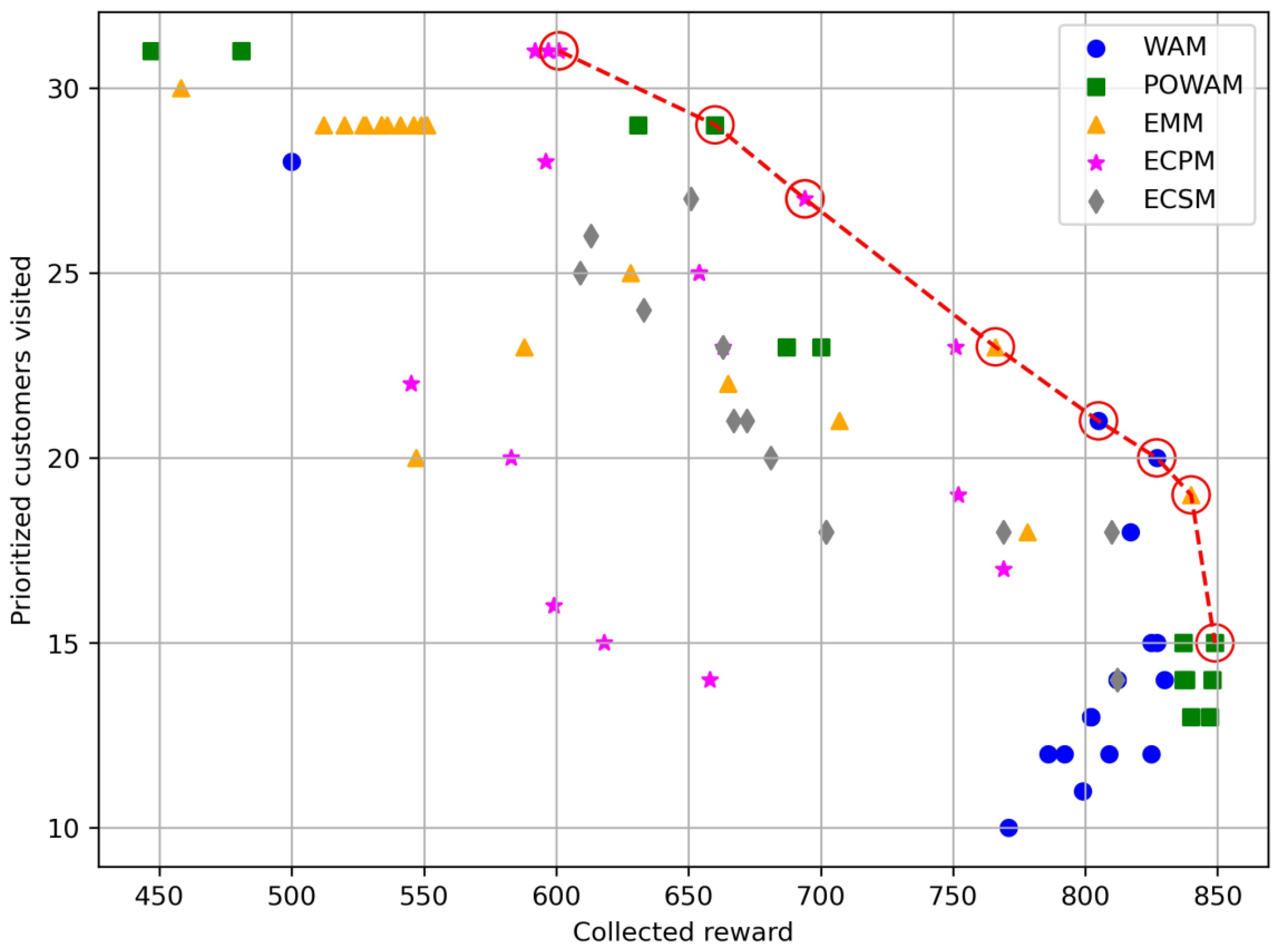
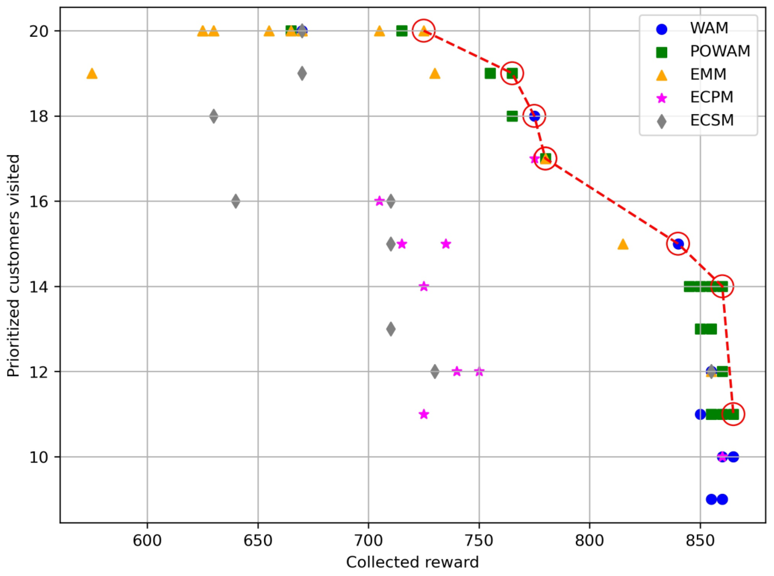
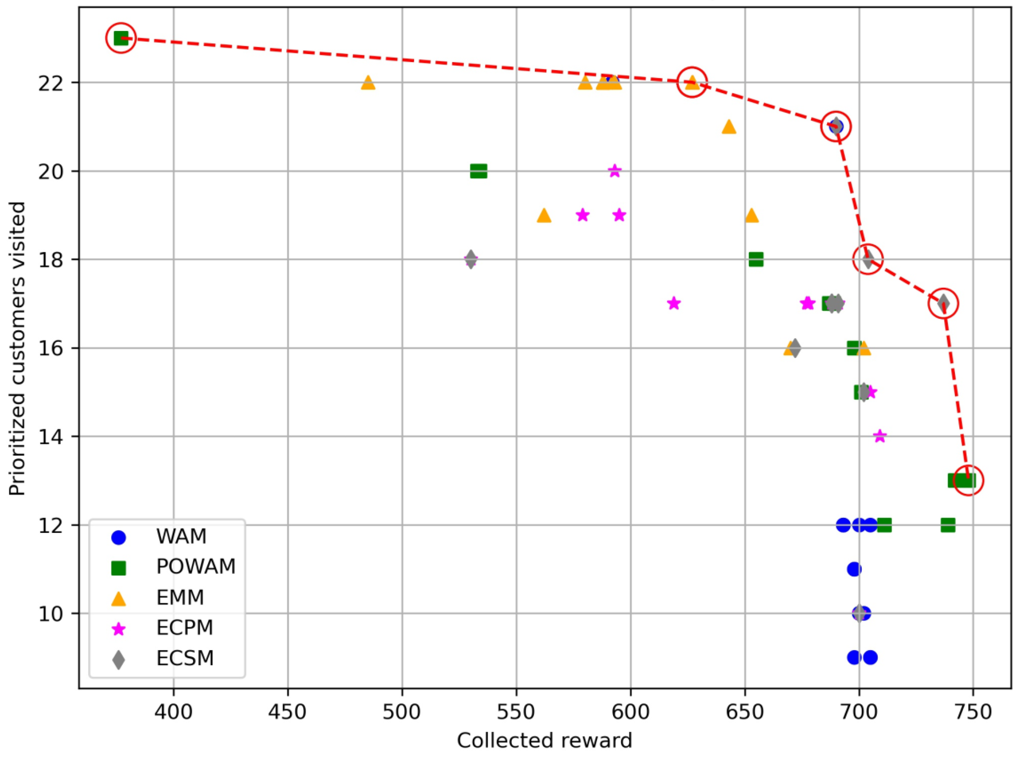
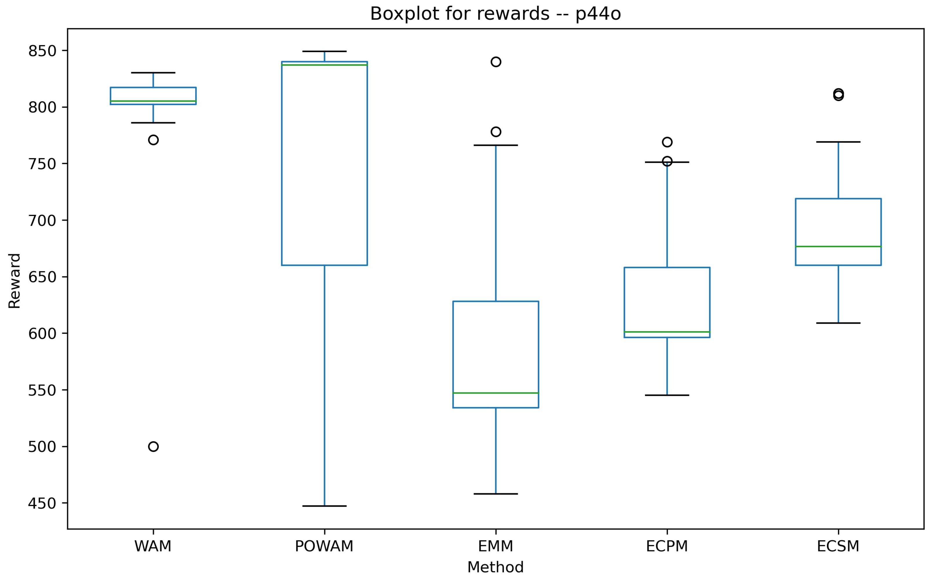
5. Computational Experiments

A comprehensive overview of the numerical instances addressed through the five previously mentioned approaches is shown in this section. The aim is to assess and compare the set of obtained solutions. All the algorithms were programmed in Python and run on a workstation with an Intel Core i 5 -11400 11th Generation and 32 GB of RAM. The maximum computational time for solving each instance is limited to 200 s. To assess the effectiveness of the proposed solution methods for the TOP, we extended to the biobjective case the widely used benchmark introduced by Chao et al. [1]. This benchmark is a standard choice in the literature for evaluating algorithms designed to address the classical version of the TOP. It is categorized into seven subsets, totaling 320 instances in total, each identified by the nomenclature p a . b . c . Here, a denotes the subset identifier, b signifies the number of vehicles, and c represents the maximum driving range. In our experiments, we choose three of the seven subsets and add a new attribute to each instance related to the priority of the node. This is performed by selecting as a ‘prioritized node’ one out of three nodes in the list of nodes. Moreover, when tackling instances that share the same network, our selection was given to those with the greatest number of available vehicles, exactly b = 4 vehicles. We exclusively considered instances possessing a ‘sufficient’ driving range, ensuring the capability to reach the farthest node in each instance. This selection strategy guarantees a diverse and representative set of scenarios for a comprehensive evaluation of the proposed solution approaches.
In a multiobjective optimization scenario, distinct, and sometimes competing, objectives must be optimized simultaneously. The primary aim is to discover a set of solutions representing Pareto optimal solutions, i.e., solutions where no single objective can be enhanced without compromising another. The solutions obtained for each instance are shown using a Pareto frontier for the different values of the coefficient η employed in the case of the POWAM and the WAM (Equation (11)), the different values of ε considered in the ECM (Equation (13)), and the EMM (Equation (14)). The abscissa axis represents the reward obtained and the ordinate axis represents the number of priority nodes visited. From the Pareto frontier, the decision-maker will be able to select the best solutions according to his/her utility function, taking into account the combination of reward values and priority nodes visited. As expected, the achieved reward decreases as more prioritized nodes are forced to be visited in the solution and vice versa. Notice that the first example, p4.4.c, has a total of 100 nodes, including the two depots, from which 33 are prioritized nodes. Similarly, the second instance, p5.4.c, has a total of 66 nodes, including depots, from which 21 are prioritized. The last instance, p7.4.c, has 102 total nodes, and 34 of them are priority nodes. For each instance, parameter c was varied in two ways, where the unique difference between cases is tmax, where tmax is the maximum time allowed by each vehicle in the fleet to complete a route.
In order to illustrate the routes traveled in each of the solutions obtained, the following graphs are presented. Specifically, for instance, for p5.4.r, we display the routes obtained with the EMM for ε = 43 and ε = 129 , corresponding to the restriction (14), in Figure 2. Additionally, routes related to the POWAM are depicted in Figure 3 for η = 0.1 and η = 0.5 in Equation (11).
The WAM and the POWAM were executed with λ 0.1 , 1 , corresponding to the normalized (POWAM) and not-normalized (WAM) biobjective functions, respectively. One of the purposes of reward weighting is to balance the two elements that form the multiobjective function. Table 1, Table 2 and Table 3 display the numerical results for some of the selected examples. For each instance and method, the obtained reward and the PN are shown for the solution corresponding to each η or ε . These solutions are also represented in Figure 4, Figure 5, Figure 6, Figure 7, Figure 8 and Figure 9. Additionally, the Pareto frontiers, which consist of the best solutions regardless of the method, are highlighted in red. Specifically, Figure 4 and Figure 5 pertain to the results in Table 1, Figure 6 and Figure 7 correspond to Table 2, and Figure 8 and Figure 9 depict the results in Table 3.
The main purpose of this work is to provide a framework for comparing five different multiobjective approaches. Let us remark that when looking at the Pareto frontiers, all five methods provide, at least in some of the examples, the best solution. Note that the extreme values of the frontiers could be assimilated as solutions to single-objective optimization problems. The points located on the left side of the graphs maximize the total number of prioritized nodes visited, while those on the right side maximize the total reward. It can be observed that the ECSM contributes more to the Pareto frontier of examples p7.4.c (Figure 8 and Figure 9), whose fundamental difference with respect to the other examples is that the maximum time per route is greater and the distribution of the nodes in the XY plane is more uniform. However, in the examples corresponding to p5.4.c, whose route time is the smallest of the examples studied, the POWAM is the one that provides the best results and therefore the one that contributes the most points to the Pareto frontier in Figure 6 and Figure 7. Finally, in Figure 4 and Figure 5, it is observed that all methods contribute to the Pareto frontiers, with the exception of ECSM, which might require a longer routing time. As a consequence, we cannot determine a dominant method with respect to the others, as they all contribute to the Pareto frontiers of the different examples. Therefore, it is up to the user to choose the method to be used depending on the objectives to be achieved. Furthermore, for a better comprehension of the variability of the results with the different methods here implemented, the values are shown by the box plots in Figure 10 and Figure 11. To facilitate the visualization of the data distribution, the values of rewards and priority nodes visited are shown separately in Figure 10 and Figure 11, respectively. Example p4.4.o. is taken as a reference, being the results obtained with the other examples similar.
It can be observed that there are some methods whose solutions offer more variability compared with the others. This tool is intended to assist the customer’s decision making in choosing which method to use for the resolution of their particular problem, depending on whether they want to obtain a wider range of solutions or not. We can observe in Figure 10 that the medians are very close to the first or third quartile, depending on the method. However, for the boxplot of priority nodes (Figure 11), a more balanced distribution is observed for the WAM, ECPM, and ECSM.

6. Conclusions and Future Work

The present study has analyzed the Multiobjective Team Orienteering Problem with a focus on prioritized nodes. Several distinct multiobjective optimization methodologies have been considered: the Weighted Average Method, the Ponderate Weighted Average Method, the epsilon-constraint method, and the Epsilon-Modified Method. This paper compares their efficacy in maximizing rewards obtained from visited nodes while optimizing the total number of prioritized nodes visited. In order to carry this out, a series of computational experiments on an extended version of popular TOP instances has been carried out. The Pareto frontiers generated by these methodologies illustrate the inherent trade-offs between the rewards accrued and the number of prioritized nodes visited, providing decision-makers with a spectrum of solutions catering to varying preferences and constraints.
The Weighted Average Method and its weighted counterpart POWAM demonstrated their aptitude in providing solutions with distinct trade-offs between the number of prioritized nodes visited and the rewards obtained. The POWAM, in particular, exhibited greater variability in solutions, offering a range of possibilities for decision-makers to explore based on their objectives. In parallel, the epsilon-constraint method introduced a constraint-based approach, allowing for the exploration of solutions where one objective was maximized while the other stayed within predefined epsilon values. Finally, the Epsilon-Modified Method maximized both values, adding a new relaxed constraint depending on epsilon. These methods showcased alternative solutions based on epsilon values, presenting a diversified set of trade-offs between rewards and prioritized nodes visited. A weighting factor of λ = 0.1 has been employed in this study, demonstrating the effectiveness of reward weighting in samples with high rewards. An area worth exploring further would be the utilization of variable weighting factors tailored to the characteristics of the data in each example. Additionally, investigating how to incorporate this reward weighting into the ECM and EMM algorithms could be beneficial. Our comparative analysis signifies that the choice of the most suitable method for addressing the MO-TOP with prioritized nodes is contingent upon the decision-makers’ specific preferences, goals, and constraints. Each method has distinct strengths and trade-offs, offering a range of solutions that cater to different optimization priorities.
This paper focuses on the deterministic version of the MultiObjective TOP, considering a generalization where the time of movement along each edge is invariant and is given by the Euclidean distance. Considering a more realistic scenario, this MO-TOP can be specified to use dynamic time, in which the travel time of each vehicle is measured in real time, allowing the incorporation of unexpected events. Some research lines that can be explored further are the following ones: (i) the integration of machine learning techniques, such as reinforcement learning, with traditional optimization algorithms could offer novel approaches to solve dynamic instances of the MO-TOP; (ii) addressing practical constraints, such as time windows, traffic congestion, vehicle capacities, and dynamic node prioritization, can render the models more applicable to real-world scenarios, making solutions more feasible and adaptable; (iii) evaluating the applicability of MO-TOP models in diverse sectors such as logistics, transportation, emergency response, and telecommunications can provide valuable insights into specific use case scenarios, enabling tailored solutions for real-world challenges; and (iv) the consideration of environmental impacts, such as reducing carbon emissions or optimizing routes for energy efficiency, could be integrated into MO-TOP models to address sustainability concerns.

Author Contributions

Conceptualization, A.A.J., L.A.-A. and S.O.-C.; methodology, L.A.-A., N.G. and S.O.-C.; software, A.A.J., L.A.-A., N.G. and S.O.-C.; formal analysis, L.A.-A. and N.G.; writing—original draft preparation, L.A.-A., S.O.-C., A.L. and N.G.; writing—review and editing, A.A.J. All authors have read and agreed to the published version of the manuscript.

Funding

This work has been partially funded by the Spanish Ministry of Science and Innovation (PID2022-138860NB-I00 and RED2022-134703-T).

Institutional Review Board Statement

Not applicable.

Informed Consent Statement

Not applicable.

Data Availability Statement

All required data is contained in the manuscript.

Conflicts of Interest

The authors declare no conflicts of interest.

Nomenclature

NSet of intermediate nodes: i , j N = 1 , 2 , , n
N Set of nodes including the initial and final depots: N = 0 , 1 , 2 , , n + 1
ESet of edges connecting the nodes: E = ( i , j ) / i , j N , i j
GGraph of the network, G = ( N , E )
DSet of homogeneous vehicles d D
t i j Travel time for each edge, t i j = t j i > 0 , i , j N
t m a x Maximum travel time for each vehicle or route
u i Reward of the node i N
x i j d Binary variable whose value is equal to 1 if vehicle d traverses edge ( i , j )
y i d Position of the node i in the tour made for the vehicle d
z i Binary variable whose value is equal to 1 if node i is priority
λ Weight for pondering the rewards in the biobjective function
α Convex linear combination constant in the efficiency value
γ Convex linear combination constant in the biefficiency value
η Convex linear combination constant in the biobjective function
s i j Time-based savings associated to the edge ( i , j ) , s i j = t i ( n + 1 ) + t 0 j t i j
e i j Efficiency value associated to the edge ( i , j ) , e i j = α s i j + ( 1 α ) ( u i + u j )
b i j Biefficiency value associated to the edge ( i , j ) , b i j = γ e i j + ( 1 γ ) ( z i + z j )
ε Deviation from the optimal value for the secondary objectives, ε > 0
P N Total number of priority nodes being visited

References

  1. Chao, I.M.; Golden, B.L.; Wasil, E.A. The team orienteering problem. Eur. J. Oper. Res. 1996, 88, 464–474. [Google Scholar] [CrossRef]
  2. Golden, B.L.; Levy, L.; Vohra, R. The orienteering problem. Nav. Res. Logist. 1987, 34, 307–318. [Google Scholar] [CrossRef]
  3. Gunawan, A.; Lau, H.C.; Vansteenwegen, P. Orienteering Problem: A survey of recent variants, solution approaches and applications. Eur. J. Oper. Res. 2016, 255, 315–332. [Google Scholar] [CrossRef]
  4. Gunawan, A.; Ng, K.M.; Kendall, G.; Lai, J. An iterated local search algorithm for the team orienteering problem with variable profits. Eng. Optim. 2018, 0273, 1–16. [Google Scholar] [CrossRef]
  5. Vansteenwegen, P.; Souffriau, W.; Van Oudheusden, D. The orienteering problem: A survey. Eur. J. Oper. Res. 2011, 209, 1–10. [Google Scholar] [CrossRef]
  6. Panadero, J.; Juan, A.A.; Bayliss, C.; Currie, C. Maximising reward from a team of surveillance drones: A simheuristic approach to the stochastic team orienteering problem. Eur. J. Ind. Eng. 2020, 14, 485–516. [Google Scholar] [CrossRef]
  7. Gosavi, A. Simulation-Based Optimization; Springer: Berlin/Heidelberg, Germany, 2015. [Google Scholar]
  8. Archetti, C.; Hertz, A.; Speranza, M.G. Metaheuristics for the team orienteering problem. J. Heuristics 2007, 13, 49–76. [Google Scholar] [CrossRef]
  9. Ke, L.; Archetti, C.; Feng, Z. Ants can solve the team orienteering problem. Comput. Ind. Eng. 2008, 54, 648–665. [Google Scholar] [CrossRef]
  10. Vansteenwegen, P.; Souffriau, W.; Berghe, G.V.; Van Oudheusden, D. A guided local search metaheuristic for the team orienteering problem. Eur. J. Oper. Res. 2009, 196, 118–127. [Google Scholar] [CrossRef]
  11. Vansteenwegen, P.; Souffriau, W.; Berghe, G.V.; Van Oudheusden, D. Iterated local search for the team orienteering problem with time windows. Comput. Oper. Res. 2009, 36, 3281–3290. [Google Scholar] [CrossRef]
  12. Souffriau, W.; Vansteenwegen, P.; Berghe, G.V.; Van Oudheusden, D. A path relinking approach for the team orienteering problem. Comput. Oper. Res. 2010, 37, 1853–1859. [Google Scholar] [CrossRef]
  13. Tricoire, F.; Romauch, M.; Doerner, K.F.; Hartl, R.F. Heuristics for the multi-period orienteering problem with multiple time windows. Comput. Oper. Res. 2010, 37, 351–367. [Google Scholar] [CrossRef]
  14. Souffriau, W.; Vansteenwegen, P.; Vanden Berghe, G.; Van Oudheusden, D. The multiconstraint team orienteering problem with multiple time windows. Transp. Sci. 2013, 47, 53–63. [Google Scholar] [CrossRef]
  15. Verbeeck, C.; Sörensen, K.; Aghezzaf, E.H.; Vansteenwegen, P. A fast solution method for the time-dependent orienteering problem. Eur. J. Oper. Res. 2014, 236, 419–432. [Google Scholar] [CrossRef]
  16. Vidal, T.; Maculan, N.; Ochi, L.S.; Vaz Penna, P.H. Large neighborhoods with implicit customer selection for vehicle routing problems with profits. Transp. Sci. 2016, 50, 720–734. [Google Scholar] [CrossRef]
  17. Paolucci, M.; Anghinolfi, D.; Tonelli, F. Field services design and management of natural gas distribution networks: A class of vehicle routing problem with time windows approach. Int. J. Prod. Res. 2018, 56, 1154–1170. [Google Scholar] [CrossRef]
  18. Estrada-Moreno, A.; Ferrer, A.; Juan, A.A.; Panadero, J.; Bagirov, A. The Non-Smooth and Bi-Objective Team Orienteering Problem with Soft Constraints. Mathematics 2020, 8, 1461. [Google Scholar] [CrossRef]
  19. Ruiz-Meza, J.; Brito, J.; Montoya-Torres, J.R. A GRASP to solve the multi-constraints multi-modal team orienteering problem with time windows for groups with heterogeneous preferences. Comput. Ind. Eng. 2021, 162, 107776. [Google Scholar] [CrossRef]
  20. Sankaran, P.; McConky, K.; Sudit, M.; Ortiz-Peña, H. GAMMA: Graph attention model for multiple agents to Solve team orienteering problem With multiple depots. IEEE Trans. Neural Netw. Learn. Syst. 2022, 34, 9412–9423. [Google Scholar] [CrossRef]
  21. Panadero, J.; Juan, A.A.; Ghorbani, E.; Faulin, J.; Pagès-Bernaus, A. Solving the stochastic team orienteering problem: Comparing simheuristics with the sample average approximation method. Int. Trans. Oper. Res. 2023. [Google Scholar] [CrossRef]
  22. Wattanasaeng, N.; Ransikarbum, K. Model and Analysis of Economic- and Risk-Based Objective Optimization Problem for Plant Location within Industrial Estates Using Epsilon-Constraint Algorithms. Computation 2021, 9, 46. [Google Scholar] [CrossRef]
  23. Mohammadi, T.; Sajadi, S.M.; Najafi, S.E.; Taghizadeh-Yazdi, M. Multi Objective and Multi-Product Perishable Supply Chain with Vendor-Managed Inventory and IoT-Related Technologies. Mathematics 2024, 12, 679. [Google Scholar] [CrossRef]
  24. Nikoubin, A.; Mahnam, M.; Moslehi, G. A relax-and-fix Pareto-based algorithm for a bi-objective vaccine distribution network considering a mix-and-match strategy in pandemics. Appl. Soft Comput. 2023, 132, 109862. [Google Scholar] [CrossRef]
  25. Shojatalab, G.; Nasseri, S.H.; Mahdavi, I. New multi-objective optimization model for tourism systems with fuzzy data and new algorithm for solving this model. Oper. Res. Soc. India 2022, 59, 1018–1037. [Google Scholar] [CrossRef]
  26. Elmi, Z.; Li, B.; Liang, B.; Lau, Y.; Borowska-Stefańska, M.; Wiśniewski, S.; Dulebenets, M.A. An epsilon-constraint-based exact multi-objective optimization approach for the ship schedule recovery problem in liner shipping. Comput. Ind. Eng. 2023, 183, 109472. [Google Scholar] [CrossRef]
  27. Banerjee, A.; Pradhan, S.; Misra, B.; Chakraborty, S. A Guide to Meta-Heuristic Algorithms for Multi-objective Optimization: Concepts and Approaches. In Applied Multi-Objective Optimization; Springer Nature: Singapore, 2024; pp. 1–19. [Google Scholar]
  28. Memarian, S.; Behmanesh-Fard, N.; Aryai, P.; Shokouhifar, M.; Mirjalili, S.; Romero-Ternero, M. TSFIS-GWO: Metaheuristic-driven takagi-sugeno fuzzy system for adaptive real-time routing in WBANs. Appl. Soft Comput. 2024, 155, 111427. [Google Scholar] [CrossRef]
  29. Evers, L.; Glorie, K.; van der Ster, S.; Barros, A.I.; Monsuur, H. A two-stage approach to the orienteering problem with stochastic weights. Comput. Oper. Res. 2014, 43, 248–260. [Google Scholar] [CrossRef]
  30. Estrada-Moreno, A.; Savelsbergh, M.; Juan, A.A.; Panadero, J. Biased-randomized iterated local search for a multiperiod vehicle routing problem with price discounts for delivery flexibility. Int. Trans. Oper. Res. 2019, 26, 1293–1314. [Google Scholar] [CrossRef]
  31. Panadero, J.; de Armas, J.; Currie, C.S.; Juan, A.A. A simheuristic approach for the stochastic team orienteering problem. In Proceedings of the 2017 Winter Simulation Conference (WSC), Las Vegas, NV, USA, 3–6 December 2017; pp. 3208–3217. [Google Scholar]
Figure 1. A basic schema of the multiobjective TOP considered in this paper.
Computation 12 00084 g001
Figure 2. Graph for the instance p5.4.r with the EMM.
Computation 12 00084 g002
Figure 3. Graph for the instance p5.4.r with the POWAM.
Computation 12 00084 g003
Figure 4. Pareto frontier for the MO-TOP p44o.
Computation 12 00084 g004
Figure 5. Pareto frontier for the MO-TOP p44r.
Computation 12 00084 g005
Figure 6. Pareto frontier for the MO-TOP p54q.
Computation 12 00084 g006
Figure 7. Pareto frontier for the MO-TOP p54r.
Computation 12 00084 g007
Figure 8. Pareto frontier for the MO-TOP p74q.
Computation 12 00084 g008
Figure 9. Pareto frontier for the MO-TOP p74r.
Computation 12 00084 g009
Figure 10. Solutions for the MO-TOP p44o using all the described methods for rewards.
Computation 12 00084 g010
Figure 11. Solutions for the MO-TOP p44o using all the described methods for priority nodes visited.
Computation 12 00084 g011
Table 1. Numerical results of instances p44o and p44r.
Instance p44o
Reward_WAMP_nodes_WAMReward_POWAMP_nodes_POWAMReward_EMMP_nodes_EMMReward_ECPMP_nodes_ECPMReward_ECSMP_nodes_ECSM
5002844731840196501470218
8052148131778186081670218
8272048131766235991670218
8171848131707217441781018
8271566029665227391976918
8251563129628256722167221
8301468723588235622068120
8121470023536295312166721
7991168723520297082366323
7711083715551296872466323
8021384915528296542563324
7861283715547206672560925
8021384814549296143161326
7921283714534296003165127
8121483814551295973181214
8091283715527296003181214
802138471345830
825128471353429
802138471354629
802138401351229
812148371454129
Instance p44r
Reward_WAMP_nodes_WAMReward_POWAMP_nodes_POWAMReward_EMMP_nodes_EMMReward_ECPMP_nodes_ECPMReward_ECSMP_nodes_ECSM
6043157031989225721886123
8872763631918239012186123
8872763631871289022286123
9032861333830299012186123
9432082529777309002286123
9482183329759297482491822
9652190026735297192574426
9471783329680287512973424
9472290026592318193079626
9461890026545318193078826
9511689423587318672875127
9471790224594318883170328
9511688124561318633073229
9471793017532318342164930
972179311957631 94717
947179332264731
947179092162531
947179162064131
954179181957931
947179002362531
947179231751331
Table 2. Numerical results of instances p54q and p54r.
Instance p54q
Reward_WAMP_nodes_WAMReward_POWAMP_nodes_POWAMReward_EMMP_nodes_EMMReward_ECPMP_nodes_ECPMReward_ECSMP_nodes_ECSM
5351953519795126451464013
7951258019795126951363513
7951257019725146901463014
7951258019740146751562015
7951258019645156501859016
7951258019600166501859517
7901268016570196501859518
7951275514535196002058019
795127851253519
780117951253519
795127851253519
795127851253519
775117851153519
795127851253519
770127851253519
770127701253519
795127701253519
770107851153519
770107801053519
795127801153519
795127851253519
Instance p54r
Reward_WAMP_nodes_WAMReward_POWAMP_nodes_POWAMReward_EMMP_nodes_EMMReward_ECPMP_nodes_ECPMReward_ECSMP_nodes_ECSM
6702066520855127501273012
7751871520815157251171013
8401571520780177401271015
8501471520730197251471016
8601171520725207351564016
8551275519665207151563018
8601175519705207051667019
8551276518575197751767020
8551376519625208601085512
8609780176252086010
86510860146302086010
855128551465520
865108451467020
860118601263020
860118501367020
855128501462520
860108551163020
850118601162520
85598551162520
86098551367020
865108651162520
Table 3. Numerical results of instances p74q and p74r.
Instance p74q
Reward_WAMP_nodes_WAMReward_POWAMP_nodes_POWAMReward_EMMP_nodes_EMMReward_ECPMP_nodes_ECPMReward_ECSMP_nodes_ECSM
4962037723742157081769917
7041653320702167081769917
7001453420685176891569917
7001465518630176321769917
7001465518628186531969917
6971468717591206381867518
7331365518591206261966519
7331368917584206402073313
733136871761920
733136871760720
733136891760720
733136981660720
733136981659120
733137011560720
733137011560720
733137111260720
733137481360720
733137391260720
733137421360720
733137471358420
Instance p74r
Reward_WAMP_nodes_WAMReward_POWAMP_nodes_POWAMReward_EMMP_nodes_EMMReward_ECPMP_nodes_ECPMReward_ECSMP_nodes_ECSM
5922237723702167051567216
6902153320670166881770215
6931253420643217091468817
6931265518653196781768817
6931265518562196771768817
6981168717627226911769117
6981165518627225301853018
6981168917593226191773717
7001068717580225951970418
698968717588225791969021
7051268917588225932070010
7001069816627227001070010
7001269816592227001070010
700106981658822
693127011558822
702107011558822
700107111258822
700107481358822
70597391258822
70597421348522
700107471358822
Disclaimer/Publisher’s Note: The statements, opinions and data contained in all publications are solely those of the individual author(s) and contributor(s) and not of MDPI and/or the editor(s). MDPI and/or the editor(s) disclaim responsibility for any injury to people or property resulting from any ideas, methods, instructions or products referred to in the content.

