

Detecting Overlapping Communities Based on Influence-Spreading Matrix and Local Maxima of a Quality Function

Finnish Defence Research Agency, Tykkikentäntie 1, P.O. Box 10, 11311 Riihimäki, Finland
Computation 2024, 12(4), 85; https://doi.org/10.3390/computation12040085
Submission received: 12 January 2024
/
Revised: 16 April 2024
/
Accepted: 18 April 2024
/
Published: 22 April 2024
(This article belongs to the Special Issue Computational Social Science and Complex Systems)
Abstract
:Community detection is a widely studied topic in network structure analysis. We propose a community detection method based on the search for the local maxima of an objective function. This objective function reflects the quality of candidate communities in the network structure. The objective function can be constructed from a probability matrix that describes interactions in a network. Different models, such as network structure models and network flow models, can be used to build the probability matrix, and it acts as a link between network models and community detection models. In our influence-spreading model, the probability matrix is called an influence-spreading matrix, which describes the directed influence between all pairs of nodes in the network. By using the local maxima of an objective function, our method can standardise and help in comparing different definitions and approaches of community detection. Our proposed approach can detect overlapping and hierarchical communities and their building blocks within a network. To compare different structures in the network, we define a cohesion measure. The objective function can be expressed as a sum of these cohesion measures. We also discuss the probability of community formation to analyse a different aspect of group behaviour in a network. It is essential to recognise that this concept is separate from the notion of community cohesion, which emphasises the need for varying objective functions in different applications. Furthermore, we demonstrate that normalising objective functions by the size of detected communities can alter their rankings.
1. Introduction
Community detection has been one of the primary applications of network science [1]. In a network, a community is a group of nodes that are more likely to be connected if they share common characteristics. In the social context, individuals in a community tend to interact more with each other than with people outside the community. Community detection is used not only in social network analysis but also in other areas of complex network analysis, such as computer, information, and biological networks. Community detection methods have been applied to analyse functional groups in various areas of biology. For instance, functional groups in metabolic networks correspond to biochemical reaction cycles or pathways. In a protein–protein interaction network, communities indicate groups of proteins that exhibit similar functionality within a biological cell [2,3].
Numerous methods and algorithms have been proposed for community detection. Most of these methods rely on the notion that nodes within a community are more strongly connected than between nodes in other communities [4,5]. However, this definition is not specific, which results in many computational approaches being available. The definition of what constitutes a community is not well posed, making community detection a challenging task [1].
Some of the earliest algorithms for dividing a network into communities include the minimum-cut method, the Girvan–Newman method, hierarchical clustering, and modularity maximisation. In the minimum-cut method, the network is divided into a predetermined number of groups selected to minimise the number of edges between groups. The Girvan–Newman algorithm identifies links in a network that connect communities based on a betweenness measure and removes them, leaving only the communities themselves [6]. Hierarchical clustering methods group similar objects into clusters and build a cluster hierarchy. Modularity is often used in community detection methods to measure the strength of a network’s division into communities [7,8,9]. By comparing the number of links within communities to what is expected by chance, modularity allows us to identify significant community structures [2,3].
When modelling network structures [10], it is important to describe the network’s topology in terms of nodes and the connections between them. These connections can be represented as directed links between neighbouring nodes, and they have weights [8,11] that indicate their ability to convey information or influence. When modelling the spread of information or influence, we also have to consider network flow models. These models describe the rules by which information or influence propagates from one node to another throughout the network [12,13,14]. In this study, we are particularly interested in non-conserved network processes, where the spread from one node continues to all adjacent nodes. In conserving flows, paths cannot be divided, whereas non-conserving flows allow propagation through multiple paths simultaneously. The relevant literature on network flow models and message passing on complex networks includes works such as [13,15].
We have developed a method to detect non-overlapping and overlapping communities in a network using a probability matrix and local maxima of a quality function (objective function). Our approach enables us to treat the exploration of network models and community detection models as distinct tasks. In our study, we model network flow using an influence-spreading model and define a community cohesion measure as the quality function. We consider communities as divisions of the network where the quality function has a local maximum.
We have designed a technique to identify groups of nodes that tend to belong to the same community frequently, based on a detailed network structure of nodes and links between them. Although some of these groups may be considered distinct communities according to our definition, not all of them are entirely self-contained communities. We use the term "building block" to describe such groups [16], as a similar concept has been used in the literature [17]. We define a community as a local maximum solution of the quality function, while building blocks are the union of detected communities and their intersections. Communities can be made up of one or more building blocks, and a building block can be a self-contained community or not. The definition of a community is quite general, and it also allows for hierarchical and overlapping communities [10,18,19,20,21,22]. Our approach, which involves searching for local maxima of the quality function, is well suited for identifying complex and overlapping community structures.
Community detection methods aim to accurately identify communities within a network while maintaining computational efficiency. While smaller networks pose no issues for computational efficiency, larger networks often require a trade-off between accuracy and efficiency. In our study, we define communities using a quality function which ensures accuracy by accepting only optimal solutions. However, the exhaustive optimisation of the quality function over the set of all graphs in a network can be computationally expensive [8]. To ensure that our simulation algorithm effectively detects the most significant communities, traditional methods such as gradient descent or simulated annealing can be employed [23,24]. These methods guarantee a similar performance to the algorithm that uses modularity as a quality function. However, the focus of this study is on presenting the modelling principles rather than using traditional methods. Our objective is to offer a complete list of identified communities rather than just the most important ones. Although various approximate techniques [25,26,27,28] can enhance the efficiency of community detection algorithms, these methods are not ideal for searching overlapping communities, as we aim to identify accurate communities and their building blocks. However, approximate techniques can still be used to initiate the search algorithm. We offer guidelines for optimising the search for overlapping communities in Appendix C.2. These hints apply to both random and optimised initialisations of the searching algorithm based on the probability matrix. The effectiveness of our influence-spreading model, which is used to construct the probability matrix, has already been discussed in [29].
In this study, experiments are carried out on multiple small networks and two moderate-size networks that consist of 5000–10,000 nodes. The results show that the method used in the study is both useful and valid for different network structures and moderate network sizes. With the help of the pseudo-algorithm and ideas provided in Appendix C.2, it is possible to apply our method to larger networks by making the algorithm more efficient. However, detecting overlapping communities in very large networks may require the development of new post-processing methods to present results, depending on the desired granularity of the analysis. This is because a significant number of almost similar overlapping communities can be detected in large networks. Nevertheless, our study shows that the results can be visualised easily for all network sizes. Furthermore, the method used in the study is particularly suitable for detailed network structures, as demonstrated with several small networks.
Several well-known networks are commonly used as test networks in the literature to compare the results of different community detection models. These include the Zachary’s Karate Club network, the American football games network, and the Dolphin social network. Also, the ground-truth communities are known for these networks. The Les Misérables social network is known for its information-theoretic solution. Additionally, we have tested our method on two moderate-size networks and the results have been visualised by a tool that generates the network layout independently without using any information about our community detection results. This allows for a more objective and visual verification of our results.
In Section 2, we summarise the most commonly used community detection methods in the literature. In Section 3, we present properties of our influence-spreading model, and in Section 4, we explain our model for detecting communities and their building blocks. In Section 5 and Section 6, we present a pseudo-algorithm that can be used to detect overlapping communities and discuss the accuracy and efficiency of our method. In Appendix C.2, we provide a more detailed explanation of the accuracy and efficiency of our algorithm and also suggest ways it could be further optimised. In Section 7, we introduce our models with four small social networks. In addition, we demonstrate the use of the models with two larger social media networks. In Section 8 and Section 9, we discuss the properties of our models and present conclusions of this study. In Appendix A, we provide a simple example of calculating circular effects in our influence-spreading model. In Appendix B, we have an example with one of our small networks of how to use the model to divide a network into three communities. In Appendix C, we discuss how to improve the efficiency of our simulation program for detecting overlapping community structures.
2. Related Work
Communities are groups of nodes in a network that are strongly connected or that share similar features or roles [1]. Detecting communities are useful in studying the structure of complex systems such as social, information, and biological networks. The applications of these methods are numerous, including epidemic spreading, market segmentation, criminal detection, influence spreading, fake news detection, recommendation systems, and more. Various articles have reviewed and discussed community detection methods [1,4,5,28,30,31,32,33,34,35], including those that consider overlapping communities [10,19,36,37].
Community detection methods aim to enhance the accuracy of the outcomes while also creating computationally efficient algorithms for various applications. The accuracy of the results is evaluated based on the algorithm’s ability to identify ground-truth communities or recover known communities that are planted in artificial benchmark networks [37,38]. Many community detection algorithms aim to optimise a quality function, such as modularity or the one proposed in this study, which measures the quality of potential communities. The development of community detection algorithms is dependent on the desired community characteristics and the computational efficiency requirements. The methods proposed often prioritise the speed of calculation, which is why multi-step algorithms are frequently utilised [39]. In such cases, the algorithm determines the connection to the community definition indirectly.
The exhaustive optimisation of a quality function over the set of all graphs of a network is computationally hard as the computational complexity of the problem is NP-complete [8]. The optimisation of the quality function proposed in this study can be compared with the corresponding optimisation of the modularity measure. As mentioned in [8], practical methods make use of approximate optimisation schemes such as greedy algorithms [25], simulated annealing [26,27,30,40], spectral methods [28], and genetic algorithms [27]. Simulated annealing [23] is a probabilistic technique that approximates the global optimum of a given function. It is preferred over exact algorithms like gradient descent [23] or branch and bound [24] when finding an approximate global optimum is more important than finding a precise local optimum within a fixed amount of time. However, using simulated annealing for large network problems is not practical because it requires a significant computational effort [7,8]. A recent study discussed in [41] proposes an effective hybrid community detection method to enhance the quality of detected communities. It aims to increase the modularity of a community detected by any detection algorithm and network structure.
Challenges and opportunities of community detection methods have been discussed in [36]. One approach is to choose a metric that measures the quality of a community and then try to maximise it. Another approach is statistical inference, where a generative model is fitted to the observed network data. One popular generative model is the stochastic block model, where nodes are grouped into blocks and edges are randomly placed between them based on their block assignments. However, this approach has a weakness in that it treats nodes within the same block as statistically independent, which may result in lower and higher-degree blocks rather than traditional community structures [36]. According to the study in [10], traditional quality measures are not enough to assess communities in a network. The study suggests that understanding the structural properties of how nodes are organised is crucial. The research in [10] investigates four quality functions: overlapping normalised mutual information [37,42], the Omega index [37], modularity [7], and the statistical F1-score.
The Louvain method [43,44], InfoMap [40], and spectral clustering [28] are three popular algorithms used for community detection. The Louvain and InfoMap methods are particularly efficient for detecting communities in large complex networks. The Louvain method uses modularity [7] as a quality function, and the algorithm optimises modularity by moving nodes between communities iteratively until no further improvements can be made. It has been shown that modularity suffers from a resolution limit, which means that in large networks, methods based on modularity would fail to detect small communities [9,44]. InfoMap, on the other hand, uses the so-called map equation to represent information diffusion on a map, where nodes are connected if they are close in the map’s representation [40]. Communities are identified by minimising the entropy of the map. Spectral clustering is a method that uses the eigenvectors of the network’s graph Laplacian matrix, which is constructed from the network’s adjacency matrix, to identify different communities within the network [2,3].
Traditionally, community detection methods have assumed that nodes belong to disjoint communities, but real-world networks often exhibit overlapping community structures where nodes can participate in multiple groups. Methods and algorithms for detecting overlapping communities have been studied in [18,20,21,22,45,46,47] to mention a few. An overlapping community detection method in complex networks based on information theory was presented in [20]. A method to analyse and explore the main statistical features of the sets of overlapping communities was presented in [18]. The first algorithm that finds simultaneously both overlapping communities and the hierarchical structure in complex networks was introduced in [21]. Later, overlapping and hierarchical community detection for weighted networks was studied, for example, in [22].
Recently, different approaches and strategies to detect and analyse overlapping communities have been proposed. In [45], the algorithm identifies similar seed communities and calculates the similarity between the neighbouring nodes and the community. Nodes that meet the similarity threshold are selected, and an adaptive optimisation function is used to expand the community. Finally, free nodes are divided into communities. The study in [46] presents two community detection algorithms that use extended modularity and cosine functions as quality functions.
One area of research involves fuzzy overlapping community detection [48,49]. In this method, each node is assigned to a community with a belonging factor that reflects the strength of its association. This fuzzy assignment can be turned into a crisp overlapping assignment by setting a belonging threshold. In a crisp overlapping assignment, each node is associated with each community with a binary belonging factor. This approach enables the identification of overlapping nodes at different scales.
Researchers have also developed tools for higher-order network analysis. Such higher-order interactions [50] have been observed in a variety of systems, including collaboration networks, ecosystems, social networks, and nervous systems. The authors in [51] found that the existence of higher-order interactions obscured the community structure in the network, and they suggested removing higher-order interactions to improve the accuracy of community detection.
The topic of opinion dynamics has received significant attention in the literature, and several studies have been conducted in [12,52,53,54]. In [54], complex contagion is defined as a situation where an individual needs several exposures before adopting an innovation or behaviour change. Unlike a disease that can spread after just one contact (simple contagion) with an infected neighbour, innovation may not spread as easily [54].
In the following section, we briefly describe our influence-spreading model, which generates an influence-spreading matrix capturing the network structure and spreading probabilities between all node pairs on the network. The model was introduced in previous research [16,29]. An alternative to the influence-spreading model is the network connectivity model [16,29], which describes the static connectivity in a network structure. In this case, the results are presented in the same matrix form, but we call the matrix a probability matrix. In Section 4, we introduce our community detection model and the corresponding pseudo-algorithm for detecting overlapping communities. The algorithm is based on a quality function that is a function of the influence-spreading matrix.
Because the influence-spreading matrix includes information on both the structure of the network and the influence-spreading process, the quality function also has similar properties. Thus, our proposed community detection method that incorporates information about the network structure into the quality function can be a solution to the problem mentioned in [10].
3. Influence-Spreading Model
Social influence can be represented by a probability matrix describing how people in a social network interact. This matrix can be created using different methods such as influence-spreading and connectivity models. To describe influence spreading, we require a network flow model to explain how influence spreads between nodes through paths in the network structure. The primary objective of our influence-spreading model is to calculate the probabilities of the influence between all individual nodes in the network by utilising the given probabilities between neighbouring nodes in the network structure [16,29,55].
Our model uses as the initial information the topological structure of the network and directed link weights for all edges between adjacent nodes in the network. The topological structure is expressed as a list of directed links between the nodes in the network. Link weights are expressed as probability values in the range from 0 to 1. Similarly to link weights, nodes can have node weights. Node and link weights indicate the ability of these network elements to disseminate the influence in the spreading process.
We use probabilistic methods because they ensure the unambiguous interpretation of the influence-spreading matrix itself and the possibility of defining further interpretative quantities of the model. An element of the influence-spreading matrix is the probability of influence from one node to another node through all alternative paths in the network. The link weight between adjacent nodes i and j is interpreted as the probability of transmitting a piece of information or exerting social influence from node i to node j. Notice that link weights are directed and can all differ between neighbouring nodes in the network structure.
The model of network flow determines how interactions within the network structure influence the spreading process. The spreading mechanism can depend on various factors, such as the network structure, link and node properties, and the nodes’ states. In this study, the node state refers to the probability of the node being influenced already. In two extreme cases of our influence-spreading model, the full breakthrough influence and network connectivity models, the node states do not affect the spreading process. However, we do consider the influence spreading through different alternative paths to a target node, following the rules of probability theory to avoid double-counting. Unique in our influence-spreading model is the method of combining the alternative paths coming from different routes from source nodes to target nodes. In the case of full breakthrough effects, we can perform this calculation analytically.
Different models can have restrictions for alternative paths. There are two extreme cases: one model allows all possible paths, including circular and recurrent paths, while the other model only allows self-avoiding paths, where nodes can only appear once. Our influence-spreading model is an example of the first case. Self-avoiding paths are commonly used for modelling virus epidemics, where infected and recovered individuals achieve full immunity to the disease. These kinds of models are also useful for describing the transmission of well-defined information on social networks and other related applications.
Spreading processes are based on the principle that spreading from a node is only possible if the influence has already reached that node. This leads to an attenuating propagation because the node and link weights are typically less than one, and they are multiplied in the probabilistic calculations. Unlike typical Markov chain or random walk models in the literature, our non-conserved model allows a spread to all possible adjacent nodes in the network within the limits of the node and link weights.
Influence spreading and network connectivity models are related, as the connectivity of nodes in a network can be considered as a limiting case of influence spreading without any recurrent or circular effects. We discussed this in our earlier paper [56]. In the following, we categorise our influence-spreading model with full breakthrough effects as a complex contagion and the network connectivity model as a simple contagion model. These definitions are generalisations of the commonly used concepts in the literature [57]. Both models consider all possible paths of the network structure limited by the network size or maximum path length parameter .
A key element of our influence-spreading model is combining the effects of different paths in the network structure [29]. When influence propagates through multiple paths to a node, we utilise a formula from probability theory that accounts for mutually non-excluding events. This method ensures that influence from multiple neighbouring nodes is calculated only once for a given source node, rather than simply being added up. By doing so, we avoid the possibility of non-physical probabilities greater than one.
We have also published an efficient algorithm [29] for computing the spreading probabilities, or the influence-spreading matrix elements, in the case of full breakthrough effects [16,55]. For large networks, the computation time can be limited by setting a value to the maximum path length . We still use simulation methods for the network connectivity or spreading model with self-avoiding paths [58].
Full breakthrough influence does not depend on the node states and does not affect the spreading process. Our current influence-spreading model only accounts for non-influenced and influenced states, where nodes that have already been influenced and those that have forgotten their opinion are considered as one state.
4. Community Detection Model
Our objective in this study is to introduce the method of separating the modelling of network structure or network flow from the modelling of community detection. We propose a community detection approach that is based on a probability matrix or an influence-spreading matrix and local maxima of a quality function.
We denote the influence-spreading matrix by C and its elements by where s is a source node, and t is a target node in the network structure. The number of nodes in the network is N. The elements in the matrix describe directed influence probabilities between any two nodes in the network. This definition differs from other matrices used in the literature, such as the adjacency matrix and the Markov matrix [3].
Centrality measures indicate a node’s importance in the network. These metrics help study network phenomena like opinion spreading and group formation. We define two variants of centrality measures based on the influence-spreading matrix. Out-centrality measures the influence one node exerts on other nodes in the network. In-centrality measures the influence other nodes in the network have on one node. These metrics denote the mean number of influenced or influencing nodes, or probabilities, depending on the normalisation convention. We define the out-centrality of node s in network G as
and the in-centrality of node t as
In the literature, several other centrality measures [2,3] have been proposed but usually, they are not based on a consistent model where probabilistic or similar interpretations are possible.
In our model, the method for detecting communities is based on finding local maximum values of the quality function in Equation (3) computed from the influence-spreading matrix elements :
If there is a local maximum for a subset of nodes V, we infer that V is a community in network G. Our approach is an application of the general principle in applied mathematics where a local optimum of an optimisation problem is an optimal solution within a neighbouring set of candidate solutions.
Equation (3) measures the division’s strength into two factions V and of the original network G. The higher the value of q, the better the sum of the cohesion of the two communities. The value of q can be used as a quantitative measure for comparing the quality of different divisions of the network structure.
One of the key features of this model is that it can have multiple local maxima with varying strengths in the network structure. This allows for the existence of several overlapping community structures. The quality function in Equation (3) can be used to measure the quality of each division. For a division, the quality function is a sum of the terms on both factions of the network. The advantage of the method based on searching local maxima of the quality function is that it does not fix the number of nodes in the communities, unlike some other community detection or network partition methods in the literature where the number of communities is predetermined [3].
We can also express Formula (3) as
We can identify that the first two terms can be expressed with the help of out-centrality measures as
Equation (5) defines a new quantity as a measure of the influence of nodes in V and on all nodes in network G, including V and . Similarly, Equation (5) can be expressed with in-centrality measures as
The centrality measures in (1) and (2) and the community influence measure in Equations (3) and (4) are closely related, as they are all based on the same influence-spreading matrix C, ensuring their consistent definition. The sum of all matrix elements of the matrix C is a constant, and we can define as a measure of cohesion of the entire network G. From Equation (4), we see that maximising q in Equation (3) is equivalent to minimising the sum of the last two terms in Equation (4). We denote this quantity as in the following formula:
Our approach involves maximising interactions within the two factions V and of a network while minimising interactions across the two factions. As a result, the definition of the community quality function, denoted by q in Equation (3), does not have cross terms. This community quality function can be compared to the commonly used modularity measure [3,8], where networks with high modularity have dense connections between nodes within modules but sparse connections between nodes in different modules.
The quality function that is defined in Equation (3) or (4) is useful when comparing divisions within a network. However, when comparing communities in networks of different sizes, it is more appropriate to normalise the measure and take into account that the sums in Equation (3) include different numbers of links and nodes depending on the sizes of the two factions of a division. Equations (3) and (4) can be normalised by dividing the expressions by the value of , as shown in Equation (8). The value of is calculated using the formula:
where represents the number of nodes in one of the two factions of the division. The number of nodes in the other faction is . Normalised quality function values can be calculated for each division of a network as
Diagonal elements do not affect the community detection results because we calculate the influence-spreading matrix elements by assuming that the spreading process is initiated from a source node with probability one [29]. We have set the values of the diagonal elements of matrix C to zero. In Equation (8), the number of terms corresponding to the first and second sums in Equation (3) are and , respectively. Source nodes can take part in circular and recurrent spreading events, as long as these events are permitted within the network flow model. However, target nodes are not involved in such events [29]. This characteristic distinguishes our model from other models, like Markov models, that are commonly found in the literature.
Normalisation has little impact on whether a community exists within a network, but it can influence the ranking of communities. If the network is divided into two communities of unequal sizes, normalisation would assign a lower weight to that division. The decision to use normalised values or not depends on the needs of the application. In this study, we present the findings as un-normalised values, except in Table 1, where we provide normalised values in column ). It is interesting to note that the community rankings for Zachary’s Karate Club have changed in a way that follows the majority of other community detection models in the literature [3,8,20]. Specifically, the division into communities with and nodes depicted in Figure 1b has the first ranking.
We introduce a broader concept of a building block that comprises all the divisions of a network identified as local maxima of Equation (3), along with their intersections. It is worth noting that while these intersections may not be local maxima of Equation (3), many of them are. All communities qualify as building blocks, but not all the building blocks meet the criteria for being communities as defined by our method.
Figure 1 shows an example of the two strongest divisions and building blocks of communities in Zachary’s Karate Club network [59] detected by our method. In Section 7.1, we explain by example how these building blocks are detected.
Notice that the sums in Equation (3) do not include interactions between the two factions of the network. This is a simplification because in real life, communication between different communities continues, albeit the relations inside each community usually are closer and more active. On the other hand, we can assume that the cross-terms cancel out in the process of community formation, which justifies leaving the cross-terms out.
It is worth noting that the model has a specific feature whereby paths between members of the same community via the other community are included in the calculation of Equation (3). While this can strengthen cohesion within a community, the effects of directly connecting the two partitions are far more significant. Strong or dense connections between the two factions can prevent a local maximum or a subdivision into two communities.
In the literature, communities are often detected based on modularity [3,6,7], a popular quality function in community detection methods. However, modularity is not based on probabilities and, therefore, it has no direct probabilistic or physical interpretation. Modularity has the same assumption as we have in our model that the cross-terms have no effects on community formation.
We define optimal solutions to the community detection problem as divisions into two factions of the original network where q in Equation (3) has a local maximum. This means that moving a node from one community to another community decreases the value of q. We justify our model by the well-known principle of equilibrium, a condition or state in which driving forces are balanced. The probabilistic interpretation of the model enables us to define the quality function as an equilibrium state of the network.
Although the value of the quality function in Equation (3) is important, there is another aspect related to the likelihood of community formation. To address this, we introduce a second measure that indicates the probability of community formation starting from a random initial setting of nodes in the network. Our statistics are derived from the computational results that we obtain by employing a basic simulation method to search for the local maxima of the quality function. We refer to this measure as a statistical measure of community formation and denote it by f and define it for a detected community A as
We define a random setting as a situation where nodes are assigned randomly to two sets that represent the two factions of the division in a network. It is worth noting that in simulations, there is a possibility that all the nodes of the network end up in one group and the second group is empty. Equation (3) always gives this division the highest value q. However, we do not count the entire network G as a separate community. Due to this effect, the statistical community formation measure f does not add up to 100 per cent. The missing portion can be interpreted as the probability of no communities arising.
It is important to note that the quality function defined in Equation (3) does not rely on the statistical measure suggested in Equation (10). As a result, the latter should be viewed as supplementary information that emphasises the difficulties involved in defining a quality function that can accurately detect overlapping communities. The measure f in Equation (10) is based on two randomly initiated sets of nodes. However, theoretically, the order of processing nodes in Algorithm 1 affects the value of f. But it is worth mentioning that the order of processing does not affect the values of q in Equation (3) for detected communities because the algorithm only accepts optimal solutions. In this respect, there is no stability issue because optimal solutions of Equation (3) are well defined.
When exploring network structures with unknown link weights, we can still analyse the network structure by using the link weight as a parameter. In this case, the same link weight value is used for all links in the network. The results of community detection can be influenced by varying the link weight parameter. If the link weight is high, then no communities will be detected. However, if the link weight is lowered, the first division into two communities will appear. Furthermore, if the link weight is further decreased, the number of different divisions into communities will increase. The numerical value of the threshold link weight is not required in the community detection algorithm. It is a theoretical quantity that has a natural interpretation in the model. The value determines a critical point above which the cohesion of the entire network is so high that there is only one community.
| Algorithm 1 Detecting overlapping communities. |
| 1: ▷ Searches communities based on probability matrix M by maximising q (Equation (3)). |
| 2: procedure Division(control parameters, M) |
| 3: ▷ Control parameters include stopping rules for the calculation and optimisation rules |
| to initialise the simulation and control the order of processing nodes. Maximum number |
| of detected communities A and maximum number of iterations B are provided as control |
| parameters. Matrix M elements describe directed influence probabilities between all node |
| pairs. Matrix M has elements. |
| 4: |
| 5: while and no other stopping criteria are fulfilled do |
| 6: |
| 7: |
| 8: while equals and do |
| 9: or for ▷ Initiate V, random or optimised |
| 10: Calculate q |
| 11: for I = 1,N do |
| 12: ▷ The order of processing nodes can be optimised |
| 13: Calculate q |
| 14: if the value of q is higher than the previous q value then |
| 15: cycle ▷ Skip the remaining statements inside the loop |
| 16: else |
| 17: ▷ Restore |
| 18: |
| 19: end if |
| 20: end for |
| 21: ▷ The number of iterations is increased by one |
| 22: end while |
| 23: if the same division has not been detected in earlier iterations then |
| 24: ▷ The number of detected divisions is increased by one |
| 25: ▷ Save vector V to list |
| 26: ▷ Save q to vector |
| 27: end if |
| 28: end while |
| 29: for J = 1,a do |
| 30: Print to a file |
| 31: end for |
| 32: ▷ Now, the list of divisions and their quality function values are saved in a file. |
| 33: end procedure |
In practice, communities with very low values of the quality function or low formation probability are not very important. However, in general, the increasing number of possible communities indicates a low cohesion and fragility of the community. Low cohesion is a natural consequence of weak ties in the community structure. The cohesion value of a set of nodes V can be calculated as a function of the link weight by taking the sum of influence matrix elements:
This measure can be calculated for any subset of nodes in the network. Now, we can express the quality function in Equations (3) and (4) yet in another form as a sum of the cohesion values of node sets V and
Our model can only identify two separate factions of the original network G at a time. Although this may appear to be a constraint, it allows us to examine the intersections and boundaries between these divisions. By calculating the intersections of different divisions, we can more effectively detect new communities in the network structure using computational methods. Some of these intersections correspond to communities, while others do not. If the set of nodes does not form a community, the statistical community measure is zero because it is not a local maximum of the quality function. As mentioned above, we have defined the concept of network building blocks as sets of nodes that are either communities or their intersections. Intersections are potential candidates for communities as members of two or more communities.
The statistical measures can indicate how long it takes to carry out a simulation. However, in some applications, it may be sufficient to find solutions in less time instead of searching for communities that may have a higher strength based on the value of the quality function. Nonetheless, structures with high local cohesion can be of interest. Local communities can emerge when nodes in the network structure locally have many links between each other or link weights are relatively high. Communities can be formed around specific interests, often consisting of a small number of members. In this model, such a scenario would involve the network being asymmetrically divided into a large and a small group, resulting in a local maximum of the quality function in Equation (3).
Communities have a crucial aspect of stability. If we remove a node or a set of nodes from a community, it can cause the entire community to dissolve, leaving behind fewer nodes that do not form an optimal solution. We can measure the impact of removing a node or nodes by calculating the difference in the value of the quality function before and after the change. This information can be used to combine overlapping communities and reduce the number of communities. However, the combined effect of removing a set of nodes is different from the sum of the individual node-removing effects. In Section 2, we discussed fuzzy overlapping community detection, where a belonging factor indicates the strength of a node’s association with a community. This factor can be defined for one node but may not be practical if we want to maintain an optimal solution for the quality function while defining the community.
5. Algorithm for Detecting Communities
Our method involves separating the modelling process into two parts: network modelling and analysing the community structure. Algorithm 1 concerns the analysis part of the problem while the network modelling part was presented in our earlier work [16,55,58]. In the past, community detection methods combined these two steps into a single model [3,32,36]. While this approach may be beneficial for optimising traditional community detection algorithms, it can also make the two models less distinct and complicate the use of a well-defined quality function for the community detection problem.
In our approach, we can use the probability matrix for optimising the search algorithm. This is because the matrix contains the needed information about the influence strength between all node pairs in the network structure. We can test how moving a node or a set of nodes affects the quality of a division and use that information to generate a more optimal division of the network. Currently, our algorithm moves one node at a time between the two factions of the division. When no move improves the value of the quality function in Equation (3), we have detected an optimal division. The order in which we process nodes does not affect the value of the quality function, but it can affect the computing time and the order of detecting communities.
The detection of building blocks begins by searching the network structure’s optimal divisions into two factions (communities). The divisions are then sorted based on a quality function value, and the building blocks are constructed. If we consider all detected divisions, the sorting does not change the result as per our definition of a building block. However, we have the option to focus only on the most significant communities and building blocks based on our requirements in the application. Particularly, when there are numerous divisions, we want to consider only the most important cases where the quality function has a high value or focus on large communities. By default, we use the q value in Equation (3) as the quality function. Note that the cohesion value of Equation (11) can also be calculated separately for the two factions of each division.
The procedure for dividing a network structure into two factions is presented in Algorithm 1. The algorithm takes as input a probability matrix, or an influence-spreading matrix, denoted by M. The matrix contains elements, where N is the number of nodes in the network, and each element represents the probability or strength of the directed influence from one node to another. There are several methods to generate the probability matrix, but we do not discuss them in this study as they depend on the particular application. Examples of different spreading processes or network connectivity models whose results can be expressed in the matrix form can be found in references [29,58].
Apart from the probability matrix, several variables are required to control the computation. These variables determine when to stop, how to optimise the initialisation of the simulation, and how to speed up the search process for optimal solutions. In this particular study, the optimal solutions correspond to the maximal values of the quality function in Equation (3). Since we are dividing the nodes of the network into two factions, we present the solutions in the form of an N-dimensional vector V with 1’s and 0’s indicating the faction of each node.
Our model defines two communities for each division, which may overlap with other communities. By analysing these overlaps, we can identify the building blocks of communities. We define building blocks as the communities themselves and all possible intersections of the detected communities.
In some cases, a building block can be classified as a community if the quality function, denoted as q in Equation (3), attains its maximum for that specific division. This implies that moving any node would lead to a reduction in the value of q. Moreover, an optimal combination can be formed by two or more building blocks, even if they are not directly linked. To maintain consistency, we also consider these solutions as communities. This is a convention since these solutions can be removed from the set of detected optimal divisions depending on our definition of a community. It is worth noting that in some studies [44], internally disconnected communities are considered problematic.
The final step of generating the building blocks from the list of network divisions can be performed in multiple ways. One approach is to use a tool like the Gephi analysis tool or an Excel spreadsheet application. In Algorithm 1, the output of line 30 can be formatted as a comma-separated values (CSV) file, which can be imported into the Gephi analysis tool. Developing software with a programming language may be a suitable alternative if specific post-processing is needed for analysing the results. To provide a concrete example of how the Gephi tool is used, we will demonstrate the building blocks structure of the football games network in Section 7.4.
6. Accuracy and Efficiency of the Method
When selecting a community detection method, it is important to consider its efficiency for practical applications. However, it is also crucial to choose a method that provides theoretically accurate solutions for specific research problems. In this study, we prioritise focusing on the theoretical aspects of analysing community structure. Our work is based on a framework that includes detail-level network structure, overlapping and hierarchic communities, and a quality function based on a probability matrix. By modelling the detail-level network and analysing community structures, we use the probability matrix to establish the connection between the two models, which helps us to streamline the modelling process and keep it under control.
Community detection methods have traditionally focused on identifying non-overlapping communities [4]. Some benchmarking methods still focus on detecting non-overlapping communities even though some nodes may belong to multiple communities. While some benchmarking methods have been proposed to measure and compare overlapping community detection methods [37,38], this field of study is still evolving. There are many issues to address in this field of study. One of the main challenges is defining what to measure and how to compare results accurately. The current benchmarks are not designed to compare the results of overlapping community detection with communities planted in artificial benchmark networks by a given quality function. Many publicly available benchmarks use the normalised mutual information measure, which is biased [42]. Hence, we demonstrated the accuracy of our algorithm and quality function using commonly used network structures with ground-truth communities and visualisations that we compared with independently generated Gephi layouts. Our findings are in good agreement with the ground truth, literature, and visualisations.
Normalised mutual information (NMI) is a commonly used metric to evaluate the accuracy of solutions to the community detection problem. However, researchers have found that NMI is often biased and can lead to inaccurate conclusions about the best algorithm for the problem [42]. Extensive numerical tests on popular algorithms have shown that the biases in the traditional mutual information significantly affect the results [42]. Although modifications to the NMI metric have been proposed to address this issue, it is still debatable whether NMI is the best measure that can be used to assess the quality of solutions to the community detection problem.
Our approach involves detecting and comparing overlapping communities using a quality function based on the influence-spreading matrix. This matrix is generated from a detailed network model, and it considers variables like node and link weights with a probabilistic interpretation [16,55,58]. The probability matrix’s elements represent the influence strength between nodes in the network, and we define derived quantities based on this matrix. Consequently, the quality function in Equation (11) serves as a method to measure the strength of communities or other sets of nodes within the network, including the building blocks determined by the intersection of detected communities.
In Section 4, we introduced another statistical measure, denoted as f, which quantified the probability of community formation. Although this measure may require significant computation time for large networks, it serves as a theoretical example of an alternative measure to evaluate the quality of detected communities. Our method for detecting communities within a network does not rely on the statistical measure, as this measure is a byproduct of the search process. The quality function q in Equation (3), the normalised quality function Q in Equation (7), and the statistical measure f can provide different rankings for the same community (refer to Table 1 in Section 4 for an example). The normalised measure Q is calculated in proportion to the number of possible connections in the communities. We conclude that different quality functions are needed for different applications and requirements. This is also related to the fact that there is currently no widely accepted definition of a community [4].
Both versions of the quality functions q in Equation (3) and Q in Equation (7) detect the same communities, but their rankings may be different. Note that f is zero for building blocks that are not communities or optimal solutions of Equation (3). However, there is an application of community formation in which we can calculate the value of cohesion even for building blocks that are not alone detected as communities. Strengthening ties in such weakly connected building blocks can lead to community formation. On the other hand, targeting information activities to nodes that belong to interceptions of detected communities can lead to the formation of a larger community. In this way, building blocks are potential groups that can evolve into a community alone or with other building blocks or communities in the network.
Our objective is to identify the divisions within a network structure. The number and comprehensiveness of the divisions required depend on the specific application. Building blocks are determined based on the list of divisions, as outlined above. The optimisation methods employed will differ depending on whether we are searching for a couple of important divisions or a more comprehensive list. In Appendix C.2, we discuss how Algorithm 1 can be improved for the detection of a large number of divisions within a network structure.
7. Demonstrations
We showcase our technique for detecting communities and building blocks using four small network structures, namely the popular Zachary’s Karate Club social network in Section 7.1, the social network of fictional characters in Victor Hugo’s book Les Misérables in Section 7.2, the dolphin animal social network in Section 7.3, and the American football games network in Section 7.4. Additionally, we present two examples of larger networks to illustrate the typical outcomes of building blocks that cover bigger structures of the networks. These are the Facebook social circles network in Section 7.5 with 4039 nodes and a Government Facebook link network in Section 7.6 with 7057 nodes. In the following, the main focus is on detecting the building blocks based on the idea explained in Section 4.
7.1. Zachary’s Karate Club Social Network
Detecting building blocks in the network structure is accomplished in two phases. First, communities are detected as division into two factions of the network as local maxima of quality function (3). Second, we sort the divisions in descending order of the quality function values and then build up different structures using this order. Our method is capable of detecting community structures that are hierarchical or overlap. One example, as shown in Figure 1, is the set of nodes which is a subset of . Sub-communities can exist inside communities.
In Figure 2, we demonstrate our incremental procedure of detecting both overlapping and non-overlapping communities. Divisions are represented by the colours brown and blue. In Figure 2a, the nodes in set make up a community, while the rest of the network constitutes the second community. Figure 2b shows the division into two approximately same-sized communities. This network division into two communities agrees with those observed by Zachary [59], except for node 3 being misclassified.
It is interesting to note that if we increase the link weights in a network until there is only one division into two communities, the last division, where all link weights are set to , agrees precisely with the observed division where node 3 belongs to the brown-coloured division in Figure 1b and Figure 2b. This result has the interpretation that when the Karate Club’s cohesion is too high, it is not optimal to split into two separate communities. This scenario corresponds to link weights higher than . Disagreement in the club results in weaker ties, or lower link weights, between the club members. When link weights are lowered to the value of , the club splits into two factions. This result is the only solution for the model with these link weights.
On the third and fourth lines of the corresponding figures, we can observe how our model detects the building blocks. The first figure on the third line (Figure 2g) is divided into two factions according to the first figure on the first line (Figure 2a). The second figure on the third line (Figure 2h) shows the intersection of node sets and highlighted in dark green. The third figure on the third line (Figure 2i) highlights four nodes in violet because they belong to two different communities. Similarly, nodes highlighted in cyan appear in both the left and right divisions of the network in Figure 2c,d. In Figure 2k, node is highlighted in yellow because it has shifted between two divisions.
Note that the last three figures in Figure 2 on the fourth line are similar despite the different divisions still detected on the third line. When the link weights are , there are seven divisions or fourteen different communities in total. In the seventh division (not shown in Figure 2), nodes have moved to the left division compared to the previous division. However, this group of nodes was detected earlier as a building block.
Communities can be constructed using building blocks. However, not all combinations of building blocks make up a community. A building block can be a community on its own or be part of a larger community. The concept of building blocks is defined as a union of intersections of communities and detected communities. The main difference between the concepts of a community and a building block is that a building block may not be a community on its own.
It is important to note that an intersection may not be a community if we only divide the network into two factions, but it can be a community when we divide a network into three or more factions, depending on how we define the quality function in these cases. In Appendix B, we provide examples of communities detected from Zachary’s Karate Club network, where divisions into three factions are considered. For instance, in Figure A2e, nodes and 32 are detected as a community while they do not constitute a community in Figure 2.
Table 1 displays the values of the quality function q and the community formation measure f. The last two columns of the table show the number of nodes for the two factions in each division. The first division has the highest value of , and the second division has the highest value of . These are the strongest divisions according to both measures. The fourth division has a relatively high value of , but it is still much lower than the values of the first and second divisions. The sum of the values for the community formation measure is . This means that the probability of not forming a community is when the search is initiated randomly.
In all network divisions, community always remains together. However, the second division has two additional variations where a set of nodes has moved from one side to the other. It is important to note that in the remaining figures, the sets of nodes indicated by the blue and brown colours are both communities. Even though community is not directly connected to the left part of the community, it is still a part of this community. The left and right parts are connected via the second community nodes in the middle of the network, indicated by the blue colour. These connections may impact the composition of nodes or local maxima of the quality function in Equation (3).
Upon examining the results shown in Figure 2, we can observe the existence of two additional groups of nodes that always remain together. The first group comprises nodes , highlighted in red, and the second group includes nodes , marked in dark green. These groups of nodes do not break up into distinct communities and are considered core structures of communities. Identifying these sets is crucial in the analysis of community formation.
7.2. Les Misérables Social Network
Our second example is the Les Misérables social network. This network illustrates the co-occurrence of fictional characters in Victor Hugo’s book Les Misérables. Characters are linked if they appear in the same paragraph or page in the book.
In Figure 3, we present the results of our model in different scenarios. Figure 3a displays the results when the model includes loops with link weights of . Figure 3b shows the results when the model uses self-avoiding paths with link weights of .
Next, we limited the path length to , and the corresponding results are shown in Figure 3c,d. To obtain approximately the same number of solutions for communities, we increased the link weights to in Figure 3c and to in Figure 3d. Because the rule of self-avoiding paths restricts interactions, higher link weights try to compensate for the effects of fewer alternative paths on the network structure.
Finally, we introduced a new scenario to study situations where a new idea spreads in a network with established opinions. For each node n, we assigned a phenomenological node weight of , and the results of this experiments are presented in Figure 3e,f. Figure 3e illustrates the results when the model includes loops with link weights of , while Figure 3f presents the results when the model uses self-avoiding paths with link weights of . In this example, equal link weights were used to model the equilibrium state of the network and spread new ideas.
When we compare Figure 3a,b, we can observe only a minor difference between the loop and self-avoiding path models. Specifically, nodes 29 and 46 have shifted from the community indicated by the violet colour to the community indicated by the black colour. Additionally, node 34 is counted in different communities in different divisions. One explanation can be that including loops in the model can strengthen larger communities or communities with more connections. Node 12, for example, has a high degree, which means it has a significant influence on its neighbours. However, the second model in Figure 3b only considers self-avoiding paths, which means there is no circular or recurrent influence between node 12 and its neighbours.
Figure 3c,d depict a scenario where we limit the path lengths to the maximum value of . Although the main structures remain the same, more nodes appear in different divisions in both models, yet all communities are still detected. Shortening the path lengths has caused less clear boundaries between communities. The shortening of path lengths prevents circular interactions, which has a similar effect as self-avoiding paths.
Finally, Figure 3e,f simulate a situation where a new idea or innovation is spreading in the network of established opinions. These results are similar to those in Figure 3a,b with minor node-level changes. In Figure 3e, nodes 29 and 46 belong to communities indicated by the violet or black colours. However, in the basic situation shown in Figure 3a, they both belong to the community indicated by the violet colour in all detected divisions. The spread of new ideas can be affected by present opinions.
The authors in [17,42] proposed an information-theoretic method to discover building blocks in a network structure. They applied their method to the Les Misérables social network. In Figure 4, we show the information-theoretic results adapted from [17]. We follow the same colouring as in Figure 3.
We can compare the results of our model presented in Figure 3 with the results of the information-theoretic model. The results are almost identical, but there are two main differences. Firstly, in our model, the building block merged with the violet building block in the information-theoretic model, while the building block in our model merged with the turquoise building block in the information theoretical model. Secondly, in the information-theoretic model, nodes , and 49 constitute separate building blocks and are not members of larger building blocks as they are in our model. The distinction between these nodes is crucial, as they possess high degrees and therefore have a significant influence on their neighbouring nodes. In our model, nodes and 49 belong to the building blocks represented by the black, violet, and dark turquoise colours, respectively. However, node 56 belongs to different divisions of the network, and hence, it cannot be unambiguously identified to any one of those communities. This holds for our model in all scenarios and the information-theoretic model.
7.3. Dolphin Social Network
The following example is an undirected social network representing frequent associations observed among 62 dolphins living off Doubtful Sound, New Zealand, from 1994 to 2001. Dolphins are connected by edges if they are observed together more often than expected by chance. One dolphin named SN100, temporarily disappeared during the observation period. Research in [60] concluded that this event led to the community of dolphins being divided into two separate groups. Later, when dolphin SN100 reappeared, the two groups reunited.
Figure 5 displays the building blocks that make up the social network of the dolphins. The link weights used to calculate these results were and . In both cases, the first division into two groups occurred in the middle of the network with dolphins SN100, Oscar, and PL belonging to the left-hand side community. This split was consistent with what was observed in real life, with the sole exception of node SN89 [60,61].
In Figure 5a, dolphin SN100 constitutes a one-node building block because it is a member of both sides in different optimal divisions of the network. The six dolphins indicated by the dark colour are also members of both sides depending on the division. Figure 5b shows a more granular view of divisions with a lower link-weight value. Our experiment using a higher link weight of resulted in one split, where dolphins DN63, Knit, and Beescratch joined the smaller community. This outcome in part supports the conclusion regarding the role of dolphin SN100, as in real life, it was a member of the larger group.
7.4. A Network of American Football Games
Next, we examine United States college football Division I games during the regular Fall 2000 season, as outlined in [6]. Each node in the network represents a team, while links signify games played between two teams. Teams are separated into conferences, with each conference containing roughly 10 teams. Notably, games are typically played between members of the same conference, rather than between different conferences. Furthermore, teams located in close proximity to one another but belonging to different conferences are more likely to play against each other than teams located far apart.
Since the approach used in [6] employed a hierarchical clustering algorithm, independent teams and teams that played against non-conference teams were merged with the conference with which they shared the closest relationship. These outcomes can be compared with those produced by our model. Additionally, the conference structure of teams can be found in the same article, presented as a graph in Figure 6b.
In Figure 7 and Figure 6a, we present results for two different link weight values, and , respectively. These values were chosen to demonstrate two different levels of granularity in the results. Figure 7a,c,e display the three divisions in order of the quality function value of Equation (3). On the right-hand side, the corresponding building blocks are displayed incrementally as intersections of the left-hand side structures. The final Figure 7f, on the right-hand side, provides a fairly accurate representation of the structure, despite being limited by only three network divisions used to construct the building blocks.
In Figure 6a, we can observe a detailed map of the identified building blocks for link weight . As seen in the figure, almost all teams are accurately grouped with the other teams in their respective conferences. To facilitate a comparison of the results, we also included another image, Figure 6b, which displays the actual conferences of the teams on a similar network graph as the building blocks in Figure 6a.
Our model does not explicitly consider the hierarchical structure of the network. In Figure 6a, eight nodes are shown in grey colour. These nodes are the building blocks made up of only one node. Additionally, three pairs of nodes form the building blocks of just two nodes. These 14 nodes can be compared to the misclassified nodes in [6] which were assigned to an incorrect conference.
Next, we provide an example of how the Gephi tool is used to analyse and visualise the building block structure. Figure 8 illustrates this structure in the Gephi tool. The figure shows three divisions——which are ordered in descending order of the quality function value. It also shows the corresponding partitions— and —that correspond to these divisions. For instance, let us take team Brigham Young. Brigham Young belongs to the community indicated by x in the first division. It also belongs to the communities indicated by o in the second and third divisions of the network. In partition , the concatenated blue symbol corresponds to 23 nodes ( of the nodes in the network) in Figure 7f. Symbols , and are identified with the building blocks of the model in Figure 7f. From Figure 6b, we can see that Brigham Young is a member of the Mountain West conference of the eight nodes indicated by the dark brown colour. These eight nodes are in the blue building block of Figure 7f. This demonstrates that the link weight of Figure 6b provides a more granular and detailed structure compared to Figure 7. The blue nodes in Figure 7e constitute a union of Mountain West and Western Athletic conferences with a couple of exceptions. In summary, the three divisions of the network with provide six building blocks that describe the network structure quite well.
7.5. Facebook Social Circles Network
In Figure 9 and Figure 10, we present two examples of how our method can detect building blocks in larger network structures. Figure 9 shows an analysis of a Facebook friend list network [62] of 4039 nodes, while Figure 10 presents an analysis of a Government Facebook structure with 7057 nodes.
We generated the graph layouts using the Fruchterman–Reingold algorithm, which exerts a force between any two nodes and minimises the energy of the system by moving the nodes and changing the forces between them. It is worth noting that the algorithm is not specifically designed for community detection, but it can be used for the visualisation and analysis of network structures. Figure 9 depicts the detected building blocks of a Facebook network. Communities are indicated by colours and node locations were determined independently by the Fruchterman–Reingold algorithm in the Gephi software [64]. In addition, links between nodes are visualised by colours also determined by the Gephi software.
In Figure 9, we present another visualisation of the model’s output. As previously mentioned, Algorithm 1 identifies different ways of dividing a network into two factions. Each such division represents two communities. The number of discovered building blocks increases with the number of detected communities. Figure 9 illustrates the building blocks as a function of detected communities, or variable a, in Algorithm 1. In the graphs, building blocks are highlighted by different colours.
The results show that there are separate node groups that form one building block, which we can call as alliances between these groups. If these alliances are optimal solutions for the quality function in Equation (3), they also constitute a community. The same phenomenon was observed in the analysis of small networks in Section 7.1 and Section 7.2. When link weights decrease, the cohesion in the network decreases as well. As a result, these alliances can break up into smaller building blocks or communities. Examining the formation and breaking up of alliances when link weights change is one way of analysing community formation in networks.
We have arranged the results based on the quality function value in Equation (3). The first division shown in Figure 9a with represents the strongest division. The second graph, shown in Figure 9b, displays the incrementally formed building blocks for the third iteration with . To save space, we have omitted the graph corresponding to the second detected division with corresponding to a small building block. Here, we demonstrate only the formation of larger building blocks. However, in some applications, the more granular changes may also be of interest. Finally, the last graph in Figure 9f displays the results after fifty optimal solutions of Equation (3) are found. Here, we set a stopping rule for the maximum number of detected communities at in our calculation.
Some large building blocks are seen to emerge after a large number of iterations. Because the results were sorted according to the quality function value, the last solutions include communities that are weak. For instance, Figure 9d,e show that the building block which is coloured blue in the upper right corner of the image split into orange and blue building blocks at this late stage. Iteration is the first graph where all large building blocks are detected with the link value . With higher link values, the number of detected communities decreases, and thus the number of detected building blocks also decreases.
7.6. Government Facebook Network
In this example, we discuss a structure of a Government Facebook network [63]. The network consists of mutually liked Facebook pages. Nodes represent the pages and links that are mutual likes among them. The network has 7057 nodes and 89455 links.
To demonstrate the different methods of using our model, we present the detected building blocks as a function of link weight w. In Figure 10, we can observe that the number of detected building blocks decreases as the link weight increases. The cohesion of the network increases, resulting in fewer optimal solutions or communities being detected in the network.
The nodes’ colour in the figure was automatically determined by the number of nodes in building blocks by the Gephi software. This results in changing colours from image to image. As we can see, peripheral groups tend to persist as separate structures in the network. In all graphs of Figure 10, there is one large community with a high internal cohesion. For lower link-weight values, this community can also break into smaller communities.
8. Discussion
We developed a technique to identify communities and their substructures in a network structure. To do this, we used a probability matrix that measured the strength of the influence between all pairs of nodes in the network. With the help of that matrix, we defined an objective function, which served as a quality measure for communities in the network. Our approach is highly adaptable and can be used with a wide range of network models and quality functions to suit various applications.
Various network flow and network connectivity models can be used to generate the probability matrix. If the goal is to study influence spreading, the matrix is called an influence-spreading matrix [29]. If we are interested in network connectivity, the matrix is called a connectivity matrix. We use a detailed topological model of the network structure in both cases, and the links between nodes are modelled bidirectionally. Probabilistic modelling is used to define all measures with physically interpretative quantities, including centrality measures, a cohesion measure, and quality functions for community detection. These measures can be expressed as a function of time or can be calculated for a stationary state where time approaches infinity [55].
In this study, we used equal link weights to provide a clear understanding of the method’s general concepts and characteristics, such as overlapping communities, quality functions, building blocks, and cohesion. We also developed detailed models of network connectivity and influence spreading with directed link weights, which describe node-level spreading in network structures. These models [16,55,58] can be used to generate probability matrices that serve as inputs for the community detection method described in this study.
In our influence-spreading model, we calculated the quality function value by averaging the out-centrality and in-centrality values for all nodes within communities. This assumption is reasonable if the strength of social ties between individuals on average are symmetric. Our quality function does not consider the direct influence between different communities, which is also a common feature in other community detection methods [4]. Different applications may require the use of different forms of quality functions. For instance, in the case of network connectivity, a similar form to ours can be used, or a form based on the connectivity between all pairs of nodes within the candidate communities. In addition, we showed that a normalisation based on the size of communities could give communities different rankings, although the normalisation did not affect which communities were detected. That is, the existence of communities and the classification of their characteristics can be considered separately.
We illustrated our method with the Zachary’s Karate Club social network which has been used as a test network in many other studies of community detection. Another example network is the Les Misérables network, because the same network has been analysed by information-theoretic methods [17]. Therefore, these results can be compared with our results. The results of the information-theoretic model were almost similar to those provided by our model. In addition, we presented results for the dolphin social network and the American football games network. These results can be compared with the corresponding ground-truth communities and many results from other studies in the literature. Our model produced results similar to those obtained in these studies.
We tested two larger networks and found that local maxima of the quality function could be identified in the network structures, including substructures. These networks represented two different network structures of egocentric social circles and page link connections on Facebook. To visualise these lower-scale structures of the networks, we used the Gephi analysis tool [64]. Layouts of the networks were generated independently by the analysis tool, and information about detected community structures from our model was added to these graphs. In this way, we showed the usefulness and validity of our model in cases where no ground-truth communities are known.
The identified local maxima indicate groups of nodes that may consist of multiple sub-communities with lower link weights or a lower cohesion of the network. However, it should be noted that not all of these groups are communities, despite what the Gephi visualisations may suggest. Whether a group of nodes is detected as a separate community depends on whether or not it is a local maximum of the quality function. This is a crucial aspect of our model.
Our model can be used to detect the main divisions into communities as a special case, when we increase the strength of social ties or link weights. This leads to only one or few solutions for the optimal community quality function. However, if the link weights are known and interpreted as probabilities, the model can detect several overlapping communities. This is a common scenario as people usually participate in numerous social activities related to work and hobbies.
We acknowledge that there are some limitations and deficiencies in the current state of our work. While we provide some preliminary tests in Appendix C.2 and discuss some optimisation methods, the software code is not yet fully optimised. We believe that most of the optimisation can be achieved by using functions of the programming language more efficiently, which is not directly related to the method itself. In the future, producing a software product is a possible task. To pinpoint obvious optimisation targets, we provided a pseudoalgorithm in Algorithm 1. However, our method and algorithm can be compared with the widely used method of maximising modularity in other community detection methods. As the optimisation of our proposed quality function and the modularity measure [8] are similar, we conclude that the computational complexity of both methods is comparable, and similar optimisation methods can be used to improve accuracy and efficiency in both cases.
One limitation of the model is that we do not know the exact link weight value in advance, especially if we are not using a probabilistic model or empirical observations to evaluate it. One way to determine suitable link weight values is to experiment with different values. We can start with a high value and gradually decrease it until communities begin to emerge; there is no need to finish the computation. Depending on the application, we can then analyse the network with a few lower link values, as we did in this study.
The structure of the quality function is a topic of research in itself. There are different ways to consider cross-terms between two or more factions of a division, particularly in network spreading models where they may be ignored or accounted for. We justified our proposed quality function by showing that maximising the quality function was equivalent to minimising the cross-term effects in the network. This is analogous to the definition of modularity that is used in other models. In a more detailed model than the one presented in this study, some effects between communities could be included in the quality function with a lower weight, as in practice, communities are not entirely isolated and tend to interact with each other.
9. Conclusions
We proposed a new method for detecting communities and their building blocks in a network structure. This method relied on a probability matrix and local maxima of a quality function. We defined communities as optimal solutions of the quality function and building blocks as the communities themselves and all possible intersections of the detected communities. Communities were formed by combining these building blocks. The probability matrix showed the strength of influence between all pairs of nodes in the network, while the quality function measured the quality of detected communities. Our model was designed to be flexible and can be implemented with various network models and quality functions that suit different applications.
Our proposed method enables the division of the problem of identifying communities within network structures into separate, independent problems. This approach makes it possible to analyse and compare different network models while keeping the community detection model consistent. Vice versa, different community detection methods can be compared while keeping the same network model.
In our study, we found that our influence-spreading model, which included full breakthrough effects and network community connectivity models, resulted in much the same community structures and building blocks. This is primarily because our model is based on the local maxima of a quality function, which means that communities usually emerge for low link values. When link values are low, the specific network flow model has only a minor effect on spreading probabilities, except in the neighbourhood of source nodes.
We defined a measure of cohesion that was a generalisation of the quality function. This measure can analyse network structures beyond detecting communities in networks, offering a broader perspective. The measure of cohesion applies to any set of nodes, including those with high link weights. Communities and building blocks emerge when there is a decrease in cohesion in the network or a specific part of it. In real social networks, this decrease in cohesion is caused by weaker ties in social relationships, which have a clear and direct interpretation.
As has been noted in the literature, the search for communities on networks is generally not a well-defined problem. In this study, we discussed the possibility of developing separate models for network structure, network flow, and community detection. Our method of using a probability matrix was proposed as a technique to combine network models and community detection models and help specify the community detection problem more consistently. In addition, we discussed the role of quality functions and their applications in community detection methods. Quality functions can be used to specify accurate community detection methods, but the most commonly used modularity function fails to detect small communities in large networks, and many of the proposed community detection algorithms are not based on quality functions or use approximate techniques to enhance computing efficiency. In this study, we proposed a novel quality function based on the probability matrix that can be used to analyse non-overlapping and overlapping community structures. The method was demonstrated with several social networks to show its usefulness and validity.
Although the problem of detecting communities has been extensively studied in numerous scientific articles, we believe that our approach adds significant value to the ongoing discussions. Our proposed method is a novel and consistent way to detect and quantify overlapping communities and their building blocks. Our work emphasises the complexity of the community detection problem, which may have been overlooked by traditional network analysis methods that rely on simple phenomenological models, use only local information of a network, or try to detect only one or a few communities. We believe that our approach offers a possible solution to these issues.
Funding
This research received no external funding.
Conflicts of Interest
The authors declare no conflicts of interest.
Appendix A
A Simple Example of Circular Effects in the Influence-Spreading Model
Here, we provide a simple example of a network with three nodes . Three bidirectional links and connect the three nodes. We calculate the spreading probability from node 1 to node 3 in the complex contagion model, where loops are allowed, and in the simple contagion model, where loops are not allowed (only self-avoiding paths). We assume that all link weights are . In the simple contagion model, only paths and are allowed, and by the rule of non-exclusive events, we obtain . In the complex contagion case, we combine the paths . We process these paths in the descending order of the longest common prefix [29]. For the four paths mentioned above, we obtain by the rule of non-exclusive events the result in three steps. In the first step, we combine paths and and obtain . In the second step, we combine path and obtain . In the third step, we obtain . If we continue the series, we obtain more correct decimals. As expected, the probability is higher for the complex contagion case.
Our model considers paths that have path lengths of , where is a parameter of the model. This makes our model a “global” type of model when compared to some “local” models found in the literature. Typically, local detection methods build a community around a seed node and add nodes until a local optimum is reached, which is computationally efficient [1]. We developed an efficient algorithm for computing influence-spreading probabilities in [29]. Although the effects decrease rapidly as a function of path length for low link weights, computing the influence-spreading matrix elements for high link weights and large networks can be time-consuming. This is because longer path lengths must be included in the calculations. However, in community detection applications, low link weights are typical because networks with high link weights have a high cohesion where no communities are detected, as explained in this study.
Figure A1.
Illustration of the influence-spreading model with full breakthrough effects and the method of combining influence probabilities through alternative routes, using a network structure of three nodes.
Figure A1.
Illustration of the influence-spreading model with full breakthrough effects and the method of combining influence probabilities through alternative routes, using a network structure of three nodes.

Appendix B
Division into Three Communities in Zachary’s Karate Club
In Figure A2, we present the results of our community detection model for detecting three distinct communities. To obtain a division into three communities, we set the element values of the influence-spreading matrix to zero for one of the communities detected in Figure 2, indicated by the white colour in Figure A2. This scenario can be explained as communities emerging step by step, where the first division into two communities occurs first, and then one of the two communities further splits into two communities. Using this procedure, we identified two different divisions in Figure 2b, three divisions in Figure 2c, and one division in Figure 2f. However, no communities were detected corresponding to Figure 2a,d,e.
In Figure A3, we display the building blocks of the three communities deduced from Figure A2. This can be compared with the corresponding Figure 2l of the building blocks of two communities. There are minor differences concerning nodes , and 34. Node 34 is one of the central nodes, and it has moved to the other community in Figure A2b.
An alternative approach would be to assume that the three communities emerge simultaneously. To achieve this, we need to modify the quality function in Equation (3) for three communities (or to any number of communities). However, we must exercise caution because the quality function excludes an increasing number of interactions as the number of communities increases due to the omission of cross-terms. This is a common weakness in community detection methods in the literature. Nevertheless, this issue is not as relevant when dividing into two factions is considered.
Figure A2.
Communities from Zachary’s Karate Club network with link weights . Divisions into three communities are displayed with three colours. Figures (a–f) show the detected divisions in the order of the quality function values. Building blocks collected together from the above graphs are shown in Figure A3.

Figure A3.
Building blocks from Zachary’s Karate Club network with link weights .

Appendix C
Appendix C.1. An Introductory Example from the Literature
We refer to the work presented in [20] as an example of many similar studies in the literature. The authors of the article compared the same example networks of Zachary’s Karate Club, dolphin network, and college football network by using the modularity and NMI measures. They compared three community detection algorithms from the literature with their proposed community detection model for overlapping communities. These results can be compared with our results, particularly concerning the overlapping nodes predicted by the models.
For Zachary’s Karate Club network, nodes 3 and 10 were detected as overlapping nodes. In another study [6], node 3 was misclassified in an analysis of the hierarchical clustering method. We can compare these results with our results in Figure 2 for the case with link weight . Although this case has a more complex structure, node 3 remains a special case.
For the dolphin network, three nodes were detected as overlapping nodes, and this again can be compared with our complex structure in Figure 5. Finally, for the college football network, only two nodes were detected as overlapping nodes. In our study, Figure 6a shows eight single grey nodes, and two yellow and two purple nodes that can be classified as overlapping nodes.
Appendix C.2. Computing Times
In our study, we identified multiple optimal divisions of a network determined by the local maxima of Equation (3). We did not conduct LFR benchmarks with synthetic networks [38]. Such benchmarks are more appropriate for detecting a small number of communities, or their method for comparing overlapping nodes is different from our approach. Additionally, the normalised mutual information (NMI) is biased [42] and differs from our proposed measure of Equation (3). Moreover, in large networks, there is a resolution limit in optimising modularity, which would make the method fail to detect small communities [9]. Therefore, comparisons with other methods, based on modularity, may not provide informative results.
In Figure A4, we explore the impact of network sizes, detected building blocks, link weight, and optimisation methods on computing times. We experimented with four different optimisation methods for selecting the initial setting of nodes or controlling the processing order of nodes in searches. First, we computed row sum vectors and column sum vectors of the probability matrix M for each column and row, respectively. Then, we sorted the array by setting pointers from 1 to N in the array and sorted the array by setting pointers from 1 to N in the array .
We divided nodes into two sets by using one of the following four methods:
- On line 9 of Algorithm 1, we picked columns from for the iterations and then set or by using the sorted row values of M. On line 12 of Algorithm 1, we moved nodes in the order determined by vector .
- Same as method 1, but with the roles of columns and rows exchanged.
- Randomised vector V on line 12 of Algorithm 1.
- Same as method 1, but on line 12 of Algorithm 1, we moved nodes in the order of the highest change in the quality function value in Equation (3).
Methods 1 and 2 rely on the out-centrality and in-centrality values of nodes. Method 3, on the other hand, does not use matrix M’s information. Method 4 involves moving nodes between the two divisions of the network by optimising the quality function. We also explored modifying method 1 and method 2 by using vectors and , respectively, to move nodes on line 12 of Algorithm 1. This had no significant impact on computing times because out-centrality and in-centrality values are correlated. Despite their numerical values being different, typically their ordering is almost the same. In Figure A4a, the method is denoted by m and link weight by w.
From Figure A4, we can draw the following conclusions:
- Optimising the initial setting of iterations and the order of processing nodes can significantly enhance the performance of Algorithm 1 (see Figure A4a–c)
- Method 3 shows the worst performance since no optimisation is utilised. However, when used for small networks, more divisions can be detected, which significantly enhances the performance of Algorithm 1 (see Figure A4a–c).
- Combining different optimisation methods can enhance the performance of Algorithm 1 and ensure that all important divisions are detected (see Figure 3a,c).
- For larger networks, the computing time increases approximately linearly as a function of detected divisions (see Figure 3a,c,d).
Figure A4.
Computing times for example networks. Effects of network sizes, optimisation methods m, link weights w, and the number of detected communities.
Figure A4.
Computing times for example networks. Effects of network sizes, optimisation methods m, link weights w, and the number of detected communities.

It is important to note that the software code and the used functions of the programming language were not optimised. Future studies should focus on planning, developing, and testing different optimisation techniques. We can see that optimisation methods and techniques can be distinct for traditional community detection and for searching all or most of the maxima of a quality function.
References
- Fortunato, S.; Newman, M.E. 20 years of network community detection. Nat. Phys. 2022, 18, 848–850. [Google Scholar] [CrossRef]
- Barabási, A.L. Network science. Philos. Trans. R. Soc. Math. Phys. Eng. Sci. 2013, 371, 20120375. [Google Scholar] [CrossRef] [PubMed]
- Newman, M.E.J. Networks: An introduction; Oxford University Press: Oxford, UK, 2018. [Google Scholar]
- Fortunato, S.; Hric, D. Community detection in networks: A user guide. Phys. Rep. 2016, 659, 1–44. [Google Scholar] [CrossRef]
- Rosvall, M.; Delvenne, J.C.; Schaub, M.T.; Lambiotte, R. Different approaches to community detection. In Advances in Network Clustering and Blockmodeling; John Wiley & Sons Ltd.: Hoboken, NJ, USA, 2019; pp. 105–119. [Google Scholar] [CrossRef]
- Girvan, M.; Newman, M.E. Community structure in social and biological networks. Proc. Natl. Acad. Sci. USA 2002, 99, 7821–7826. [Google Scholar] [CrossRef] [PubMed]
- Newman, M.E. Modularity and community structure in networks. Proc. Natl. Acad. Sci. USA 2006, 103, 8577–8582. [Google Scholar] [CrossRef] [PubMed]
- Leicht, E.A.; Newman, M.E. Community structure in directed networks. Phys. Rev. Lett. 2008, 100, 118703. [Google Scholar] [CrossRef] [PubMed]
- Fortunato, S.; Barthelemy, M. Resolution limit in community detection. Proc. Natl. Acad. Sci. USA 2007, 104, 36–41. [Google Scholar] [CrossRef] [PubMed]
- Vieira, V.d.F.; Xavier, C.R.; Evsukoff, A.G. A comparative study of overlapping community detection methods from the perspective of the structural properties. Appl. Netw. Sci. 2020, 5, 51. [Google Scholar] [CrossRef]
- Bellingeri, M.; Bevacqua, D.; Sartori, F.; Turchetto, M.; Scotognella, F.; Alfieri, R.; Nguyen, N.; Le, T.; Nguyen, Q.; Cassi, D. Considering weights in real social networks: A review. Front. Phys. 2023, 11, 1152243. [Google Scholar] [CrossRef]
- Long, J.C.; Cunningham, F.C.; Braithwaite, J. Bridges, brokers and boundary spanners in collaborative networks: A systematic review. BMC Health Serv. Res. 2013, 13, 158. [Google Scholar] [CrossRef]
- Borgatti, S.P. Centrality and network flow. Soc. Netw. 2005, 27, 55–71. [Google Scholar] [CrossRef]
- Freeman, L.C.; Borgatti, S.P.; White, D.R. Centrality in valued graphs: A measure of betweenness based on network flow. Soc. Netw. 1991, 13, 141–154. [Google Scholar] [CrossRef]
- Newman, M. Message passing methods on complex networks. Proc. R. Soc. 2023, 479, 20220774. [Google Scholar] [CrossRef]
- Kuikka, V. Influence spreading model used to analyse social networks and detect sub-communities. Comput. Soc. Netw. 2018, 5, 12–15. [Google Scholar] [CrossRef] [PubMed]
- Riolo, M.A.; Newman, M. Consistency of community structure in complex networks. Phys. Rev. E 2020, 101, 052306. [Google Scholar] [CrossRef] [PubMed]
- Palla, G.; Derényi, I.; Farkas, I.; Vicsek, T. Uncovering the overlapping community structure of complex networks in nature and society. Nature 2005, 435, 814–818. [Google Scholar] [CrossRef] [PubMed]
- Gupta, S.K.; Singh, D.P.; Choudhary, J. A review of clique-based overlapping community detection algorithms. Knowl. Inf. Syst. 2022, 64, 2023–2058. [Google Scholar] [CrossRef]
- Zhou, H.; Zhang, Y.; Li, J. An overlapping community detection algorithm in complex networks based on information theory. Data Knowl. Eng. 2018, 117, 183–194. [Google Scholar] [CrossRef]
- Lancichinetti, A.; Fortunato, S.; Kertész, J. Detecting the overlapping and hierarchical community structure in complex networks. New. J. Phys. 2009, 11, 033015. [Google Scholar] [CrossRef]
- Prokop, P.; Dráždilová, P.; Platoš, J. Hierarchical Overlapping Community Detection for Weighted Networks. In Proceedings of the International Conference on Complex Networks and Their Applications, Menton, France, 28–30 November 2023; Springer: Berlin/Heidelberg, Germany, 2023; pp. 159–171. [Google Scholar] [CrossRef]
- Henderson, D.; Jacobson, S.H.; Johnson, A.W. The theory and practice of simulated annealing. In Handbook of Metaheuristics; Springer: Boston, MA, USA, 2003; pp. 287–319. [Google Scholar] [CrossRef]
- Land, A.H.; Doig, A.G. An Automatic Method for Solving Discrete Programming Problems; Springer: Berlin/Heidelberg, Germany, 1960; Volume 28, pp. 497–520. [Google Scholar] [CrossRef]
- Rustamaji, H.C.; Kusuma, W.A.; Nurdiati, S.; Batubara, I. Community detection with greedy modularity disassembly strategy. Sci. Rep. 2024, 14, 4694. [Google Scholar] [CrossRef]
- Yang, J.; Sun, Y.; Cheng, S.; Bian, K.; Liu, Z.; Sun, X.; Cao, Y. A Memetic Algorithm Based on Adaptive Simulated Annealing for Community Detection. In Proceedings of the International Conference on Intelligence Science, Xi’an, China, 28–31 October 2022; Springer: Berlin/Heidelberg, Germany, 2022; pp. 20–28. [Google Scholar] [CrossRef]
- Jokar, E.; Mosleh, M.; Kheyrandish, M. Discovering community structure in social networks based on the synergy of label propagation and simulated annealing. Multimed. Tools Appl. 2022, 81, 21449–21470. [Google Scholar] [CrossRef]
- Newman, M.E. Spectral methods for community detection and graph partitioning. Phys. Rev. E 2013, 88, 042822. [Google Scholar] [CrossRef] [PubMed]
- Kuikka, V.; Aalto, H.; Ijäs, M.; Kaski, K.K. Efficiency of Algorithms for Computing Influence and Information Spreading on Social Networks. Algorithms 2022, 15, 262. [Google Scholar] [CrossRef]
- Lancichinetti, A.; Fortunato, S. Community detection algorithms: A comparative analysis. Phys. Rev. E 2009, 80, 056117. [Google Scholar] [CrossRef] [PubMed]
- Mittal, R.; Bhatia, M. Classification and comparative evaluation of community detection algorithms. Arch. Comput. Methods Eng. 2021, 28, 1417–1428. [Google Scholar] [CrossRef]
- Khan, B.S.; Niazi, M.A. Network community detection: A review and visual survey. arXiv 2017, arXiv:1708.00977. [Google Scholar]
- Yang, Z.; Algesheimer, R.; Tessone, C.J. A comparative analysis of community detection algorithms on artificial networks. Sci. Rep. 2016, 6, 30750. [Google Scholar] [CrossRef] [PubMed]
- Lancichinetti, A.; Radicchi, F.; Ramasco, J.J.; Fortunato, S. Finding statistically significant communities in networks. PLoS ONE 2011, 6, e18961. [Google Scholar] [CrossRef] [PubMed]
- Hric, D.; Darst, R.K.; Fortunato, S. Community detection in networks: Structural communities versus ground truth. Phys. Rev. E 2014, 90, 062805. [Google Scholar] [CrossRef]
- Cherifi, H.; Palla, G.; Szymanski, B.K.; Lu, X. On community structure in complex networks: Challenges and opportunities. Appl. Netw. Sci. 2019, 4, 117. [Google Scholar] [CrossRef]
- Xie, J.; Kelley, S.; Szymanski, B.K. Overlapping community detection in networks: The state-of-the-art and comparative study. ACM Comput. Surv. (Csur) 2013, 45, 43. [Google Scholar] [CrossRef]
- Lancichinetti, A.; Fortunato, S. Benchmarks for testing community detection algorithms on directed and weighted graphs with overlapping communities. Phys. Rev. E 2009, 80, 016118. [Google Scholar] [CrossRef] [PubMed]
- Ding, Z.; Zhang, X.; Sun, D.; Luo, B. Overlapping community detection based on network decomposition. Sci. Rep. 2016, 6, 24115. [Google Scholar] [CrossRef]
- Rosvall, M.; Bergstrom, C.T. Maps of random walks on complex networks reveal community structure. Proc. Natl. Acad. Sci. USA 2008, 105, 1118–1123. [Google Scholar] [CrossRef] [PubMed]
- Öztemiz, F.; Karcı, A. KO: Modularity optimization in community detection. Neural Comput. Appl. 2023, 35, 11073–11087. [Google Scholar] [CrossRef]
- Jerdee, M.; Kirkley, A.; Newman, M. Normalized mutual information is a biased measure for classification and community detection. arXiv 2023, arXiv:2307.01282. [Google Scholar] [CrossRef]
- Blondel, V.D.; Guillaume, J.L.; Lambiotte, R.; Lefebvre, E. Fast unfolding of communities in large networks. J. Stat. Mech. Theory Exp. 2008, 2008, P10008. [Google Scholar] [CrossRef]
- Traag, V.A.; Waltman, L.; Van Eck, N.J. From Louvain to Leiden: Guaranteeing well-connected communities. Sci. Rep. 2019, 9, 5233. [Google Scholar] [CrossRef]
- Liu, H.; Li, Z.; Wang, N. Overlapping community detection algorithm based on similarity of node relationship. Soft Comput. 2023, 27, 13689–13700. [Google Scholar] [CrossRef]
- Hieu, D.D.; Duong, P.T.H. Overlapping community detection algorithms using Modularity and the cosine. arXiv 2024, arXiv:2403.08000. [Google Scholar]
- Shen, H.W.; Cheng, X.Q.; Guo, J.F. Quantifying and identifying the overlapping community structure in networks. J. Stat. Mech. Theory Exp. 2009, 2009, P07042. [Google Scholar] [CrossRef]
- Nepusz, T.; Petróczi, A.; Négyessy, L.; Bazsó, F. Fuzzy communities and the concept of bridgeness in complex networks. Phys. Rev. E 2008, 77, 016107. [Google Scholar] [CrossRef] [PubMed]
- Gregory, S. Fuzzy overlapping communities in networks. J. Stat. Mech. Theory Exp. 2011, 2011, P02017. [Google Scholar] [CrossRef]
- Lambiotte, R.; Rosvall, M.; Scholtes, I. From networks to optimal higher-order models of complex systems. Nat. Phys. 2019, 15, 313–320. [Google Scholar] [CrossRef] [PubMed]
- Liu, Y.; Fan, Y.; Zeng, A. Higher-order interactions disturb community detection in complex networks. Phys. Lett. A 2023, 494, 129288. [Google Scholar] [CrossRef]
- Bakshy, E.; Rosenn, I.; Marlow, C.; Adamic, L. The role of social networks in information diffusion. In Proceedings of the 21st International Conference on World Wide Web, Lyon, France, 16–20 April 2012; pp. 519–528. [Google Scholar] [CrossRef]
- Lamberson, P.J. Diffusion in Networks. In The Oxford Handbook of the Economics of Networks; Oxford University Press: Oxford, UK, 2016. [Google Scholar] [CrossRef]
- Centola, D. How Behavior Spreads: The Science of Complex Contagions; Princeton University Press: Princeton, NY, USA, 2018. [Google Scholar]
- Kuikka, V. Modelling community structure and temporal spreading on complex networks. Comput. Soc. Netw. 2020, 8, 13. [Google Scholar] [CrossRef]
- Almiala, I.; Kuikka, V. Similarity of epidemic spreading and information network connectivity mechanisms demonstrated by analysis of two probabilistic models. AIMS Biophys. 2023, 10, 173–183. [Google Scholar] [CrossRef]
- Centola, D.; Macy, M. Complex Contagions and the Weakness of Long Ties. Am. J. Sociol. 2007, 113, 702–734. [Google Scholar] [CrossRef]
- Almiala, I.; Aalto, H.; Kuikka, V. Influence spreading model for partial breakthrough effects on complex networks. Phys. A Stat. Mech. Appl. 2023, 630, 129244. [Google Scholar] [CrossRef]
- Zachary, W.W. An Information Flow Model for Conflict and Fission in Small Groups. J. Anthropol. Res. 1977, 33, 452–473. [Google Scholar] [CrossRef]
- Newman, D.; Lusseau, D. Identifying the Role That Individual Animal Play in Their Social Network. Proc. R. Soc. Lond. B 2004, 271, S477–S481. [Google Scholar] [CrossRef]
- Lusseau, D.; Schneider, K.; Boisseau, O.J.; Haase, P.; Slooten, E.; Dawson, S.M. The bottlenose dolphin community of doubtful sound features a large proportion of long-lasting associations: Can geographic isolation explain this unique trait? Behav. Ecol. Sociobiol. 2003, 54, 396–405. [Google Scholar] [CrossRef]
- Leskovec, J.; Krevl, A. SNAP Datasets: Stanford Large Network Dataset Collection. 2014. Available online: http://snap.stanford.edu/data (accessed on 1 January 2020).
- Rossi, R.A.; Ahmed, N.K. The Network Data Repository with Interactive Graph Analytics and Visualization. In Proceedings of the Twenty-Ninth AAAI Conference on Artificial Intelligence, Austin, TX, USA, 25–30 January 2015; Volume 29. [Google Scholar] [CrossRef]
- Bastian, M.; Heymann, S.; Jacomy, M. Gephi: An Open Source Software for Exploring and Manipulating Networks. In Proceedings of the International AAAI Conference on Web and Social Media, San Jose, CA, USA, 17–20 May 2009. [Google Scholar] [CrossRef]
Figure 1.
Zachary’s Karate Club network [59] with the two strongest divisions (a,b) and building blocks (c) detected by our method (building blocks are indicated by different colours).
Figure 1.
Zachary’s Karate Club network [59] with the two strongest divisions (a,b) and building blocks (c) detected by our method (building blocks are indicated by different colours).

Figure 2.
Communities and building blocks from Zachary’s Karate Club network with link weights . Figures illustrate our cumulative method to detect building blocks of the community structure. The method is based on processing the divisions of the network into two communities (figures a–f) and processing them in the descending order of the quality function value shows the building blocks of the network (figures g–l). Numerical values of the quality function q and community formation measure f are shown in Table 1.

Figure 3.
Building blocks of the Les Misérables network. The left column shows the results of our model with circular and recurrent effects while the right column shows the results of the model with paths with no visits to the same node more than once. The following are the model versions and their corresponding link weight values: (a) Loops allowed with , (b) Self-avoiding paths with , (c) Loops allowed with and maximum length , (d) Self-avoiding paths with and maximum length , (e) Loops allowed with and a new idea, (f) Self-avoiding paths with and a new idea.

Figure 4.
The results of the information-theoretic approach in [17] applied to the Les Misérables social network. The structure of building blocks maximises mutual information. The figure is adapted from [17].

Figure 5.
Building blocks of the dolphin social network calculated with link weights and .

Figure 6.
Football games network. (a) Results from our model, (b) Conferences of the teams taken from the information in [6].
Figure 6.
Football games network. (a) Results from our model, (b) Conferences of the teams taken from the information in [6].

Figure 7.
The three divisions of the network of American football games between Division IA colleges during the Fall 2000 regular season. Left-hand side figures show the divisions into two communities, and the right-hand side figures show the corresponding building blocks. Link weight value is used in the figures. Correspondence to the Gephi data table in Figure 8 is the following: (a) Division 1, (b) Partition , (c) Divison 3, (d) Partition , (e) Divison 2, (f) Partition .


Figure 8.
Screenshots from the Gephi analysis tool.

Figure 9.
Detected building blocks in the Facebook network [62]. The set of six graphs depict the results obtained through Algorithm 1, which detects an increasing number of communities over the iterations, denoted by variable a. Link weight value is used in the figures.
Figure 9.
Detected building blocks in the Facebook network [62]. The set of six graphs depict the results obtained through Algorithm 1, which detects an increasing number of communities over the iterations, denoted by variable a. Link weight value is used in the figures.

Figure 10.
Detected building blocks of the Government Facebook network [63].
Figure 10.
Detected building blocks of the Government Facebook network [63].


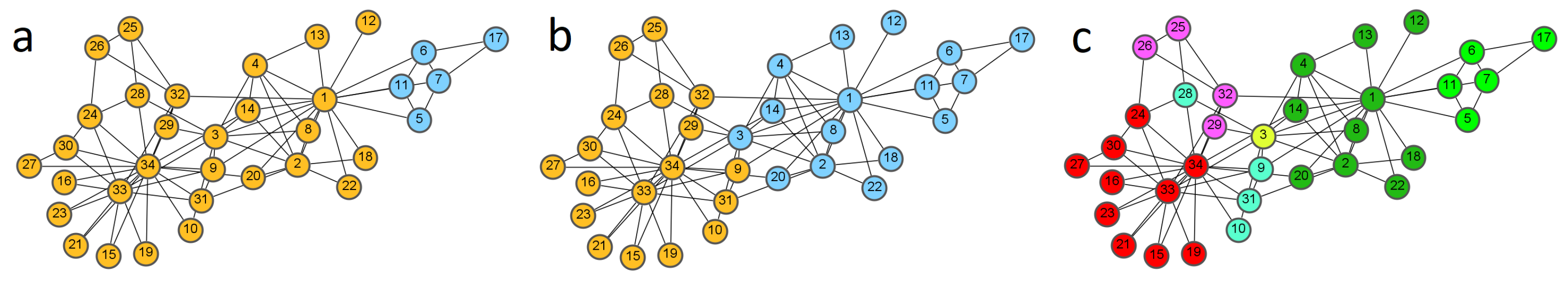
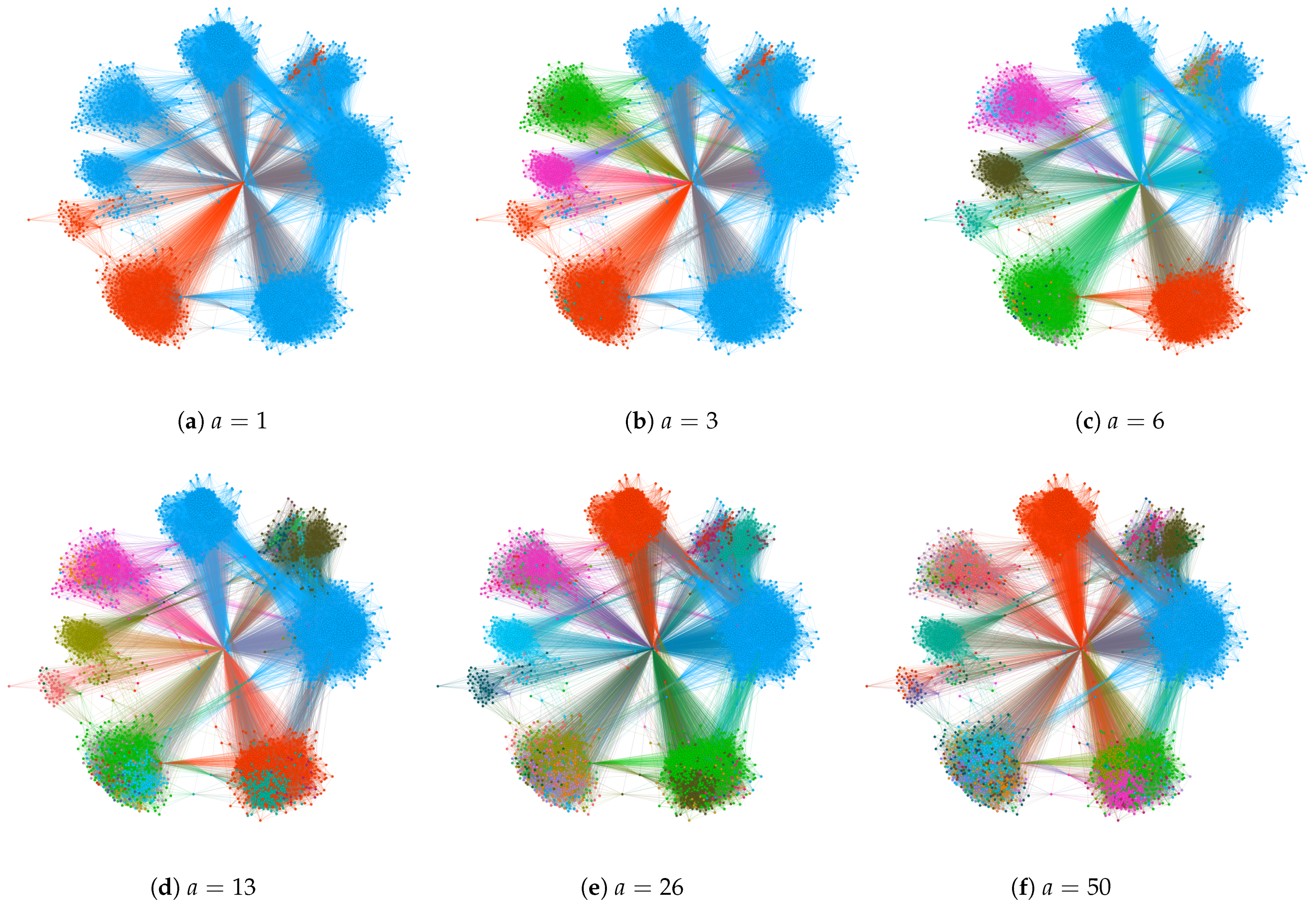
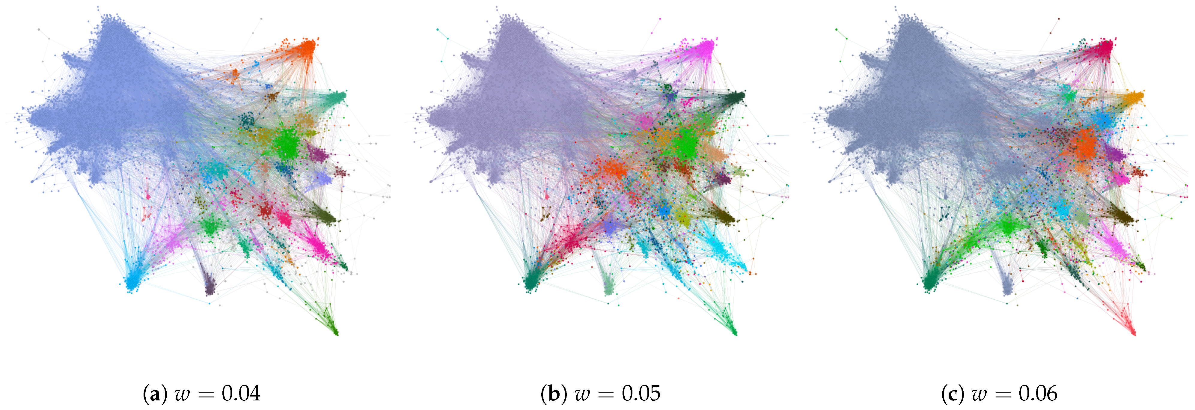
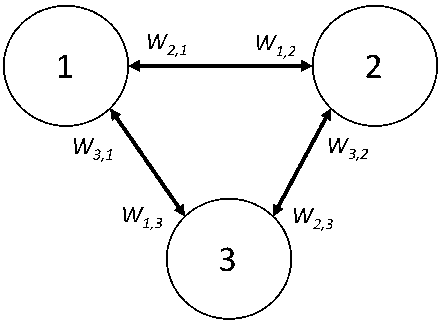
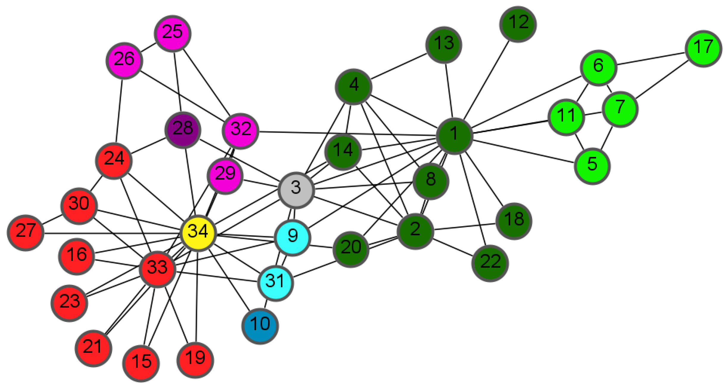
Table 1.
The values of the quality function q (un-normalised), Q (normalised by Equation (8)), and community formation measure f for the detected divisions with a link weight value in the Zachary’s Karate Club network. The last two columns show the number of nodes in the two factions in each division.
| q (%) | Q (%) | f (%) | #1 | #2 | |
|---|---|---|---|---|---|
| 1 | 10.6 | 14.1 | 10.3 | 29 | 5 |
| 2 | 9.4 | 18.7 | 12.9 | 16 | 18 |
| 3 | 8.9 | 17.3 | 2.6 | 20 | 14 |
| 4 | 8.9 | 15.2 | 5.2 | 24 | 10 |
| 5 | 8.8 | 15.0 | 1.6 | 10 | 24 |
| 6 | 8.2 | 16.2 | 0.3 | 15 | 19 |
| 7 | 8.1 | 16.0 | 0.4 | 19 | 15 |
Disclaimer/Publisher’s Note: The statements, opinions and data contained in all publications are solely those of the individual author(s) and contributor(s) and not of MDPI and/or the editor(s). MDPI and/or the editor(s) disclaim responsibility for any injury to people or property resulting from any ideas, methods, instructions or products referred to in the content. |
© 2024 by the author. Licensee MDPI, Basel, Switzerland. This article is an open access article distributed under the terms and conditions of the Creative Commons Attribution (CC BY) license (https://creativecommons.org/licenses/by/4.0/).
Share and Cite
MDPI and ACS Style
Kuikka, V. Detecting Overlapping Communities Based on Influence-Spreading Matrix and Local Maxima of a Quality Function. Computation 2024, 12, 85. https://doi.org/10.3390/computation12040085
AMA Style
Kuikka V. Detecting Overlapping Communities Based on Influence-Spreading Matrix and Local Maxima of a Quality Function. Computation. 2024; 12(4):85. https://doi.org/10.3390/computation12040085
Chicago/Turabian StyleKuikka, Vesa. 2024. "Detecting Overlapping Communities Based on Influence-Spreading Matrix and Local Maxima of a Quality Function" Computation 12, no. 4: 85. https://doi.org/10.3390/computation12040085
Note that from the first issue of 2016, this journal uses article numbers instead of page numbers. See further details here.