
BEM Modeling for Stress Sensitivity of Nonlocal Thermo-Elasto-Plastic Damage Problems

1
Department of Mathematics, Adham University College, Umm Al-Qura University, Adham, Makkah 28653, Saudi Arabia
2
Department of Basic Sciences, Faculty of Computers and Informatics, Suez Canal University, New Campus, Ismailia 41522, Egypt
Computation 2024, 12(5), 87; https://doi.org/10.3390/computation12050087
Submission received: 6 April 2024
/
Revised: 18 April 2024
/
Accepted: 19 April 2024
/
Published: 23 April 2024
(This article belongs to the Topic Advances in Computational Materials Sciences)
Abstract
:The main objective of this paper is to propose a new boundary element method (BEM) modeling for stress sensitivity of nonlocal thermo-elasto-plastic damage problems. The numerical solution of the heat conduction equation subjected to a non-local condition is described using a boundary element model. The total amount of heat energy contained inside the solid under consideration is specified by the non-local condition. The procedure of solving the heat equation will reveal an unknown control function that governs the temperature on a specific region of the solid’s boundary. The initial stress BEM for structures with strain-softening damage is employed in a boundary element program with iterations in each load increment to develop a plasticity model with yield limit deterioration. To avoid the difficulties associated with the numerical calculation of singular integrals, the regularization technique is applicable to integral operators. To validate the physical correctness and efficiency of the suggested formulation, a numerical case is solved.
1. Introduction
The non-classical heat conduction problem, which requires solving the parabolic heat equation under non-local conditions, is especially important here. A domain integral specifies the total amount of heat energy contained in the solid under consideration, resulting in the non-local state. The temperature is set in a specific section of the solid’s border using an unknown control function to be determined. Noye et al. [1], Gumel et al. [2], Dehghan [3], and many other authors have numerically addressed this problem using finite difference methods. In the non-local case, the domain integral was reduced to an integral that only included the heat flow on the solution domain’s border. The physical solution was obtained from the domain of the Laplace transformation using a computational technique for inverting Laplace transformation. Ang and Ooi [4] recently presented a boundary element technique for solving axisymmetric heat equation subject to nonlocal condition.
Continuum damage mechanics were created to fill the gap between classical continuum mechanics and fracture mechanics. Due to the presence of a fracture process zone with multiple microcracks at the fracture front, classical linear elastic fracture mechanics cannot be applied to heterogeneous quasi-brittle materials such as concrete, rocks, sea ice, fiber composites, and toughened ceramics unless very large structures are considered. Microcracking in materials eventually causes strain softening, which causes the elastic modulus matrix to become a non-positive definite, resulting in an ill-posed problem [5,6]. Finite element simulations with elasto-plastic models and yield limit deterioration in the traditional theory of plasticity produce varied findings depending on the discretization meshes [7]. The results ignore finite element mesh refinements and lead to a solution with no energy dissipation upon failure at infinite mesh refinement. To avoid this wrong behavior, localization limiters must be implemented, ensuring that the strain-softening zone has a minimum finite size [8,9,10,11,12,13]. The non-local continuum idea, which was first presented in elasticity for a different reason [14,15], is an effective localization restriction. The non-local continuum with local strain, as proposed in References [16,17], is a useful model that treats just the elements that cause strain softening as non-local while treating all other variables as local. This idea is applicable to all constitutive models [13]. Jirásek [18] investigated non-local models, whereas Baant and Jirásek [19] conducted considerable research. The boundary element technique (BEM) is an increasingly popular alternative to the finite element method (FEM). The key advantage over domain techniques is that there are fewer unknowns. It is a powerful linear elasticity technique that has also proven useful in inelastic material challenges. Swedlow and Cruse [20] developed BEM formulations for elasto-plasticity. Ricardella [21] pioneered the initial 2D study, whereas Chaudonneret [22] and Kumar and Mukherjee [23] reported the first 2D viscoplastic analyses. Banerjee et al. also contributed to this study [24]. Banerjee and Cathie provided the first axisymmetric elasto-plastic investigations, as well as the first 3D elasto-plastic applications [25]. Since then, inelastic formulations have advanced greatly [26,27,28,29]. To resolve inelastic material difficulties, the BEM solution algorithm requires precise stress rate estimation. Regularization or singularity reduction prior to numerical computation can accelerate and improve the BEM solution process.
In this study, a novel boundary element method (BEM) modeling is utilized to numerically compute the temperature field in a body containing a preset amount of heat energy. A plasticity model with yield limit deterioration based on the regularized initial stress boundary element formulation is used to deal with non-local softening damage. This formulation eliminates one source of numerical error by utilizing a regularized integral representation of stresses. The BEM approach finally reduces the problem to a system of linear algebraic equations that need to be solved at each time level. Because of the regularization or singularity reduction performed before to numerical calculation, the validity, accuracy, and efficiency of the proposed BEM formulation are demonstrated.
2. Formulation of the Problem
According to small strain theory in the Cartesian coordinate system, the thermo-elasto-plastic governing equation can be expressed as follows [30]:
where
and
Upon being subjected to the following initial, boundary, and non-local conditions,
where such that , and are suitable chosen functions.
3. BEM Modeling of the Temperature Field
Let us consider the two-dimensional region bounded by open curve with endpoints A and B on the -axis as shown in Figure 1.
By applying the divergence theorem to (12), we obtain [32]
Let begin and end at and , respectively, and select the following two points on as follows
If and are the values of temperature at and , respectively, then the boundary temperature is approximated using
where
Similarly, is approximated using
if and .
The domain integral in (24) is approximated by picking collocation points , , within the interior of . As collocation points on the element , the points and are also used. Thus, we obtain
where for , the coefficients are defined implicitly by [34]
and
Thus, we use the following approximations:
Then, from (29) and (24), we obtain
If the temperature is provided by either (10) or (11) at , then is not known. In the event where the temperature’s normal derivative is provided by (12) at , then is not known. At every inner collocation point, the temperature is unknown.
In other words, (35) represents a system of linear algebraic equations in unknown functions of if is taken to be known. (Remember that the control function , which is shown in (10), is an unidentified function that needs to be found). Therefore, the system requires one further equation to be completed.
Using (23), Equation (19) can be expressed as
where
The steps to solve the linear algebraic Equations (35) and (36) are as follows:
Step 1 Let in (35) and (36).
Step 2 Determine using the initial condition in .
Step 3 Solve the linear algebraic Equations (35) and (36) for the unknowns , and either or
Step 4 With now known and in (35) and (36),
Step 5 Solve linear algebraic Equations (35) and (36) for the unknowns and either or .
Step 6 By repeatedly letting at higher time levels, it is possible to solve for unknowns.
4. BEM Modeling of Thermo-Elasto-Plastic Deformation
The integral equation for the displacement rate is as follows [35]:
where the fundamental displacement must satisfy the following equation
As a result, we have the following boundary integral equation (BIE)
Upon substituting the displacement rate integral Equation (39) into (4) and applying regularization [36], we obtain the following stress rate integral equation
where
where is the unit vector tangent to at .
To treat a strong singularity of the kernel, the domain can be split into regular and singular parts, ; thus, we can write
With
where
The BIE (53) can be used to estimate the stress tensor rates as follows
By solving the regularized BIE [37], with using (51), we obtain
Thus, by using (51), we have the following relations
The incremental iterative solution approach will employ the regularized BIE (50) and (60) as well as the regularized BIE (53). Thus, the regular Gaussian quadrature rule has been used to calculate all the boundary and domain integrals.
The yield function can be expressed as
For the model in this study, the work-hardening function is used to characterize softening, where the hardening/softening parameter the plastic strain increment can be defined as
where .
From (62) and (64), the proportionality coefficient can be expressed as
We will consider the strain-softening von Mises plasticity model in this work because the nonlocal BEM solution will be easier and more obvious.
The stress intensity
in which
and
Thus, we obtain
where
and
The fundamental idea behind the non-local continuum is that only the constitutive equation variables that cause strain softening are non-local [7]. Spatial averaging is more computationally efficient than plastic strains
Then, the non-local scaling parameter can be defined as
where
where the non-local weight function can be expressed as [7]
where measures the material heterogeneity scale and .
After determining the non-local average , we can calculate the non-local plastic strain and stress increments as follows
The BIE (50) can be transformed into matrix form using the discretization in the BEM formulation as
The stress tensor rates can be expressed as
Thus, we can write (78) and (79) as follows
Then, the boundary unknowns are
where
By using (81) and (82), the plastic stress rate can be expressed as
where
The iteration process may be summarized as follows:
Step 1 Calculate from (84);
Step 2 Calculate ;
Step 3 Calculate from (73);
Step 4 Calculate ;
Step 5 Verify iteration convergence by comparing to the value of (84) in step 1;
Step 6 If the relative change between two subsequent iteration stages is less than the set tolerance (which is a value obtained by measuring a component’s capacity to perform its design function in the presence of a flaw or damage), return to step 1 and start a new load increment.
5. Numerical Results and Discussion
The proposed BEM strategy employed in this study can be used for a broad spectrum of thermal stress sensitivity of nonlocal thermo-elasto-plastic damage problems.
To solve the systems resulting from the BEM discretization in the current study, we employed Zan et al.’s stable communication avoidance S-step-generalized minimal residual approach (SCAS-GMRES) to reduce the number of iterations and computation time [39]. Table 1 compares the SCAS-GMRES [39], fast modified diagonal, and toeplitz splitting (FMDTS) of Xin and Chong [40] and the unconditionally convergent-scaled circulant and skew-circulant splitting (UC-RSCSCS) of Zi et al. [41] during our solution of the current problem. This table displays the number of iterations (Iter.), processor time (CPU time), relative residual (Rr), and error (Err.) calculated for various length scale parameter values (). According to Table 1, the SCAS-GMRES iterative approach uses the least amount of Iter. and CPU time, meaning that it outperforms the FMDTS and UC-RSCSCS iterative methods.
The thermal stresses , and sensitivities are compared for various softening damage parameters ( and ) concerning the differences between local and non-local theories
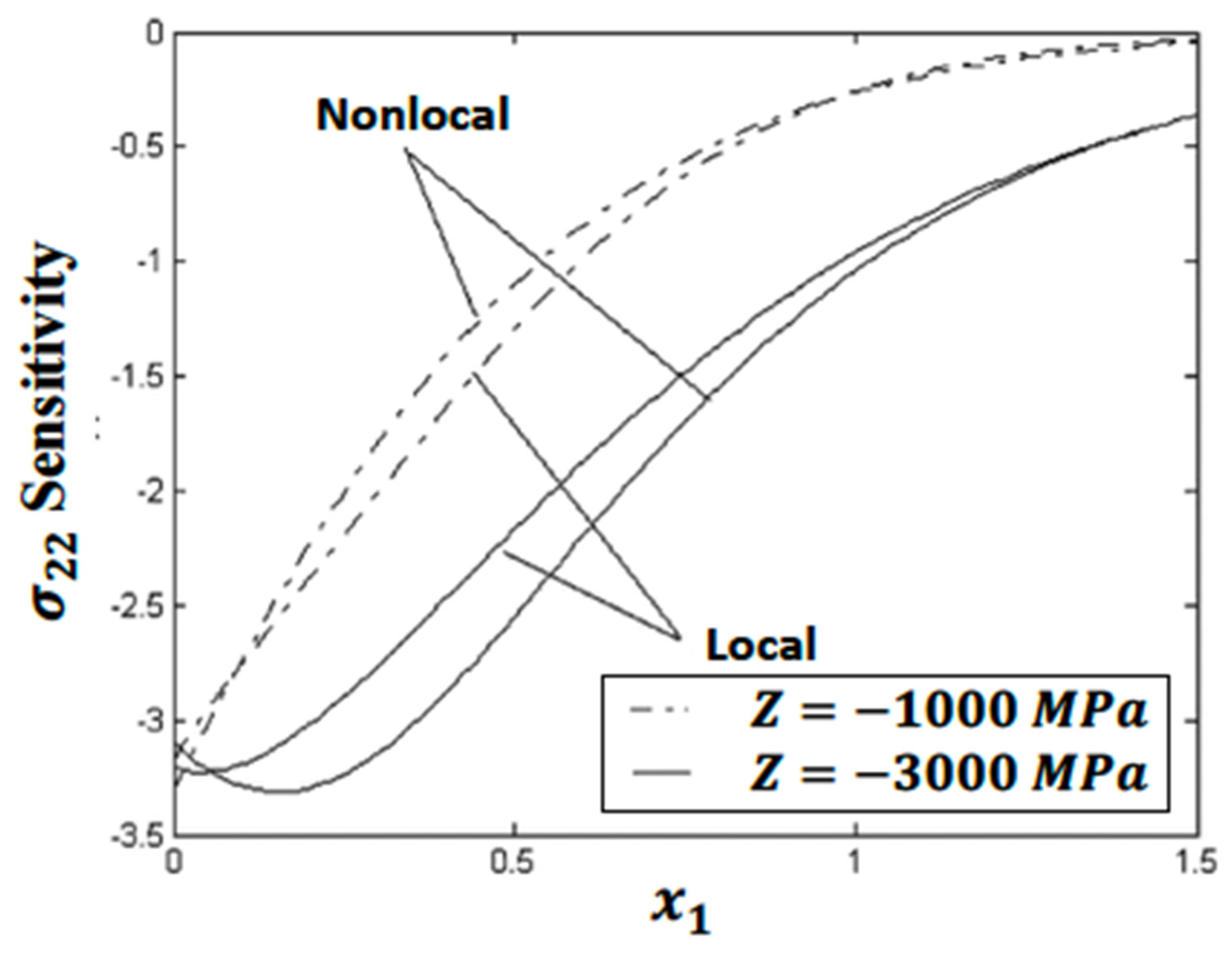
Figure 2 shows that the values of the thermal stress sensitivity based on the softening parameter are larger compared to the values based on the softening parameter for local and nonlocal theories. The values of the thermal stress sensitivity based on the softening parameters and decrease in the range and increase in the range . However, the values of the thermal stress sensitivity based on the softening parameters and converge to zero with increasing for .
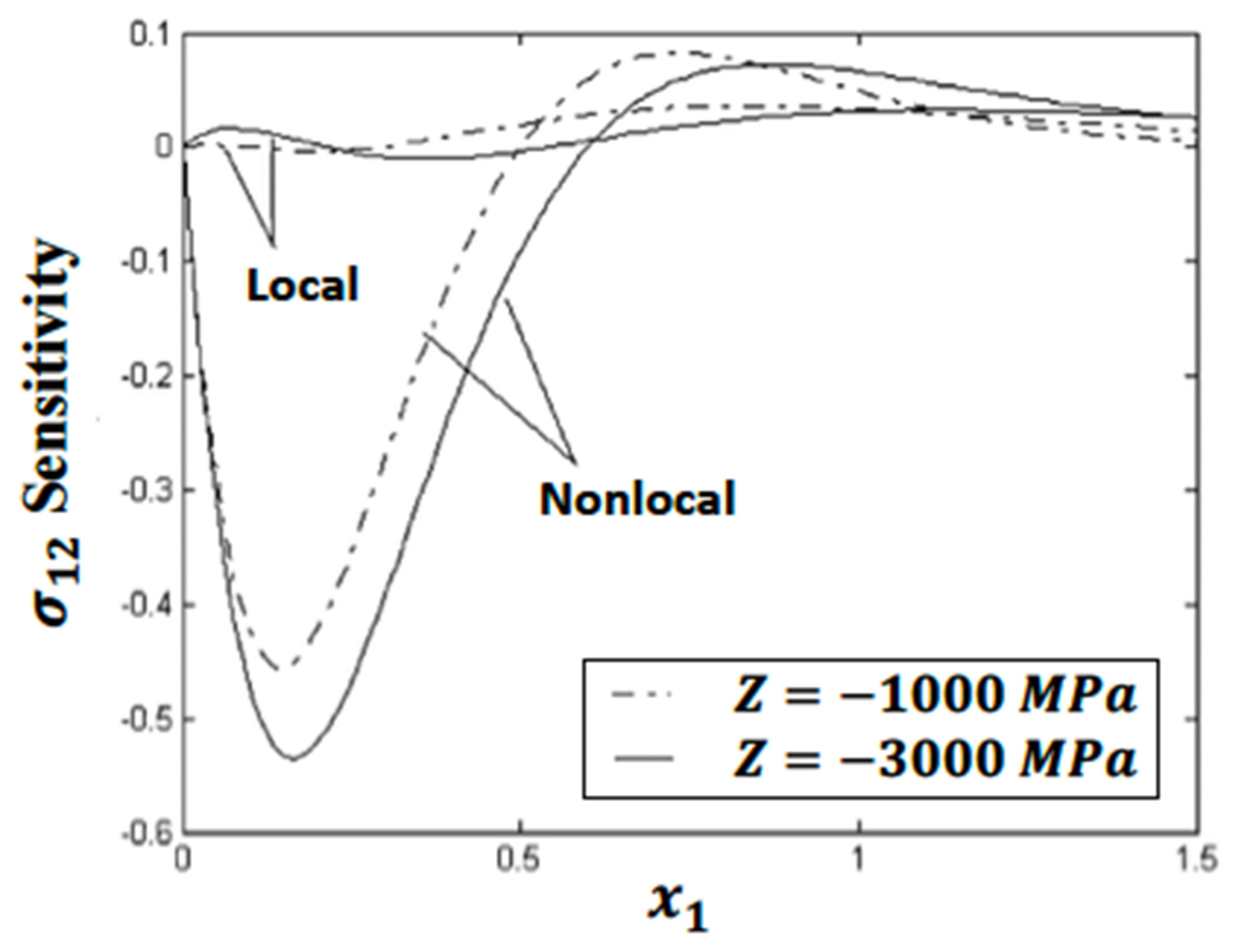
Figure 3 shows that the values of the stress sensitivity in both softening parameters and decrease in the ranges and , while increasing in the range . However, for nonlocal theory, the values of the stress sensitivity based on softening parameter increase in the range and decrease in the range , while, based on the softening parameter , decrease in the range and increase in the range . The values of the stress sensitivity based on the softening parameters and converge to zero with increasing for .
Figure 4 depicts the behavior of the values of the stress sensitivity based on the softening parameters and for local and nonlocal theories, which are similar. The values of the stress sensitivity based on the softening parameter increase in the range . However, the values of the stress sensitivity based on the softening parameter increase in the range . The values of softening parameters and converge to zero with increasing distance at .
There were no published results that supported the suggested technique’s conclusions. Some of the literature can be considered as part of the planned investigation [42,43,44,45,46]. As a result, we examined a specific instance in our research and compared our BEM results to the finite difference method (FDM) and finite element method (FEM).
Figure 5, Figure 6 and Figure 7 depict the distributions of the thermal stresses , and overtime for the current BEM, finite difference method (FDM) of Ricci and Brünig [47], and the finite element method (FEM) of Su et al. [48]. These statistics demonstrate that the BEM is in excellent agreement with the SRBNS and FEM, proving the validity and accuracy of our suggested approach. The computing results for the considered problem were obtained using Matlab R2022a on a MacBook Pro with a 2.9 GHz Core i9 processor. The boundary element technique described in this paper applies to a wide variety of nonlocal thermo-elasto-plastic damage scenarios.
6. Conclusions
The numerical solution of the stress sensitivity in nonlocal thermo-elasto-plastic damage problems is presented using a new boundary element method (BEM) model. A boundary element model is used to represent the numerical solution to the heat conduction equation under non-local conditions. The non-local condition specifies the overall quantity of thermal energy contained in the substance under examination. The approach for solving the heat equation will disclose an unknown control function that governs the temperature in a specific section of the solid’s boundary. The initial-stress BEM for structures with strain-softening damage is used in a boundary element program with iterations at each load increment to create a plasticity model with yield limit deterioration. To eliminate the challenges associated with the numerical calculation of singular integrals, the regularization technique is applicable to integral operators. A numerical scenario is used to validate the physical accuracy and efficiency of the proposed formulation.
Funding
The authors did not receive support from any organization for the submitted work.
Data Availability Statement
All data generated or analyzed during this study are included in this published article.
Conflicts of Interest
The authors declare no conflicts of interest.
Nomenclature
| Nonlocal weight function | Domain | ||
| Boundary | Work-hardening function | ||
| Dirac delta function of argument | CPV | Cauchy principal value | |
| Total heat energy | Solid specific heat capacity | ||
| Plastic strain intensity | Tensor depending on the stress tensor | ||
| Plastic strain rate | Area of an infinitesimal portion of | ||
| Plastic strain increment | Length of an infinitesimal part of | ||
| Temperature | Second kind elliptic integral | ||
| Absolute zero temperature | Effective stress | ||
| Outward normal derivative of on | Identity matrix | ||
| Solid thermal conductivity | First kind elliptic integral | ||
| Lamé elastic constants | hardening-softening parameter | ||
| Proportionality coefficient | Material characteristic length | ||
| Spatial non-local average | component unit vector normal to | ||
| Elastic stress intensity | Control function | ||
| Stress rate tensor | Solid Volume | ||
| Plastic stress rate | Cylindrical Coordinates | ||
| Elastic stress rate | S | Solid Surface | |
| Elastic stress increment | Deviator of stresses | ||
| Plastic stress increment | Traction rate | ||
| Unit vector tangent to boundary at | Fundamental displacement | ||
| Displacement rate |
References
- Noye, B.J.; Dehghan, M.; VanderHoek, J. Explicit finite difference methods for two-dimensional diffusion with a non-local boundary condition. Int. J. Eng. Sci. 1994, 32, 1829–1834. [Google Scholar] [CrossRef]
- Gumel, A.B.; Ang, W.T.; Twizell, E.H. Efficient parallel algorithm for the two-dimensional diffusion equation subject to specification of mass. Int. J. Comput. Math. 1997, 64, 153–163. [Google Scholar] [CrossRef]
- Dehghan, M. Numerical solution of a parabolic equation subject to specification of energy. Appl. Math. Comput. 2004, 149, 31–45. [Google Scholar] [CrossRef]
- Ang, W.T.; Ooi, E.H. A dual-reciprocity boundary element approach for solving axisymmetric heat equation subject to specification of energy. Eng. Anal. Bound. Elem. 2008, 32, 210–215. [Google Scholar] [CrossRef]
- Bažant, Z.P. Instability, ductility and size effect in strain softening concrete. J. Eng. Mech. Div. (ASCE) 1976, 12, 331–344. [Google Scholar] [CrossRef]
- Sandler, I.S. Strain-softening for static and dynamic problems. In Proceedings of the Symposium on Constitutive Equations: Micro, Macro and Computational Aspects; Willam, K.J., Ed.; ASME: New York, NY, USA, 1984; pp. 217–231. [Google Scholar]
- Bažant, Z.P.; Lin, F.-B. Non-local yield degradation. Int. J. Numer. Methods Eng. 1988, 26, 1805–1823. [Google Scholar] [CrossRef]
- Bažant, Z.P.; Belytschko, T.B.; Chang, T.P. Continuum theory for strain-softening. J. Eng. Mech. Div. (ASCE) 1984, 110, 1666–1692. [Google Scholar] [CrossRef]
- Bažant, Z.P. Crack band model for fracture of geomaterials. In Proceedings of the 4th International Conference on Numerical Methods in Geomechanics, Edmonton, AB, Canada, 31 May–4 June 1982; Eisenstein, Z., Ed.; pp. 1137–1152. [Google Scholar]
- Bažant, Z.P.; Ožbolt, J. Nonlocal microplane model for fracture, damage and size effect in structures. J. Eng. Mech. (ASCE) 1990, 116, 2485–2505. [Google Scholar] [CrossRef]
- Bažant, Z.P.; Ožbolt, J. Compression failure of quasibrittle material; Nonlocal microplane model. J. Eng. Mech. (ASCE) 1992, 118, 540–556. [Google Scholar] [CrossRef]
- Bažant, Z.P.; Cedolin, L. Stability of Structures; Oxford University Press: Oxford, UK, 1991. [Google Scholar]
- Bažant, Z.P.; Planas, J. Fracture and Size Effect in Concrete and Other Quasibrittle Materials; CRC Press: Boca Raton, FL, USA, 1998. [Google Scholar]
- Kröner, E. Elasticity theory of materials with long-range cohesive forces. Int. J. Solids Struct. 1967, 4, 731–742. [Google Scholar] [CrossRef]
- Eringen, A.C.; Edelen, D.G.B. On nonlocal elasticity. Int. J. Eng. Sci. 1972, 10, 233–248. [Google Scholar] [CrossRef]
- Bažant, Z.P.; Pijaudier-Cabot, G. Modeling of distributed damage by nonlocal continuum with local strain. In Proceedings of the 4th International Conference on Numerical Methods in Fracture Mechanics, San Antonio, TX, USA, 23–27 March 1987; pp. 411–432. [Google Scholar]
- Pijaudier-Cabot, G.; Bažant, Z.P. Nonlocal damage theory. J. Eng. Mech. (ASCE) 1987, 113, 1512–1533. [Google Scholar] [CrossRef]
- Jirásek, M. Nonlocal models for damage and fracture: Comparison of approaches. Int. J. Solids Struct. 1998, 35, 4133–4145. [Google Scholar] [CrossRef]
- Bažant, Z.P.; Jirásek, M. Nonlocal integral formulations of plasticity and damage: Survey of progress. J. Eng. Mech. (ASCE) 2002, 128, 1119–1149. [Google Scholar] [CrossRef]
- Swedlow, J.L.; Cruse, T.A. Formulation of boundary integral equations for three-dimensional flow. Int. J. Solids Struct. 1971, 7, 1673–1683. [Google Scholar] [CrossRef]
- Ricardella, P.C. An Implementation of the Boundary Integral Technique for Planar Problems of Elasticity and Elasto-Plasticity. Ph.D. Thesis, Carnegie-Mellon University, Pittsburgh, RI, USA, 1973. [Google Scholar]
- Chaudonneret, M. Boundary integral equation method for visco-plasticity analysis. J. Mécanique Appliquée 1977, 1, 113–131. [Google Scholar]
- Kumar, V.; Mukherjee, S. A boundary integral equation formulation for time dependent inelastic deformation in metals. Int. J. Mech. Sci. 1975, 19, 713–724. [Google Scholar] [CrossRef]
- Banerjee, P.K.; Cathie, D.N.; Davies, T.G. Two and three-dimensional problems of elastoplasticity. In Developments in Boundary Element Methods; Applied Science Publishers: London, UK, 1979; Volume 1, pp. 63–95. [Google Scholar]
- Banerjee, P.K.; Cathie, D.N. Boundary element methods for axisymmetric plasticity. In Innovative Numerical Methods for the Applied Engineering Science; Shaw, R.P., Pilkey, W., Pilkey, B., Wilson, R., Lakis, A., Chaudouet, A., Marino, C., Eds.; University of Virginia Press: Charlottesville, VA, USA, 1980. [Google Scholar]
- Telles, J.C.F.; Brebbia, C.A. Boundary elements in plasticity. Appl. Math. Model. 1981, 5, 275–281. [Google Scholar] [CrossRef]
- Henry, D.P.; Banerjee, P.K. A new BEM formulation for two and three-dimensional elastoplasticity using particular integrals. Int. J. Numer. Methods Eng. 1988, 26, 2079–2096. [Google Scholar] [CrossRef]
- Leitao, V.; Alabadi, M.H.; Rooke, D.P. The dual boundary element formulation for elastoplastic fracture mechanics. Int. J. Numer. Methods Eng. 1995, 38, 315–333. [Google Scholar] [CrossRef]
- Herding, U.; Kuhn, G. A field boundary element formulation for damage mechanics. Eng. Anal. Bound. Elem. 1996, 18, 137–147. [Google Scholar] [CrossRef]
- Balaš, J.; Sládek, J.; Sládek, V. Stress Analysis by Boundary Element Methods; Elsevier: Amsterdam, The Netherlands, 1989. [Google Scholar]
- Brebbia, C.A.; Telles, J.C.F.; Wrobel, L.C. Boundary Element Techniques, Theory and Applications in Engineering; Springer: Berlin/Heidelberg, Germany, 1984. [Google Scholar]
- Abramowitz, M.; Stegun, I. Handbook of Mathematical Functions; Dover: New York, NY, USA, 1970. [Google Scholar]
- París, F.; Cañas, J. Boundary Element Method: Fundamentals and Applications; Oxford University Press: Oxford, UK, 1997. [Google Scholar]
- Wang, K.; Mattheij, R.M.M.; ter Morsche, H.G. Alternative DRM formulations. Eng. Anal. Bound. Elem. 2003, 27, 175–181. [Google Scholar] [CrossRef]
- Sládek, J.; Sládek, V.; Bažant, Z.P. Non-local boundary integral formulation for softening damage. Int. J. Numer. Methods Eng. 2003, 57, 103–116. [Google Scholar] [CrossRef]
- Sládek, V.; Sládek, J. Non-singular boundary integral representation of stresses. Int. J. Numer. Methods Eng. 1992, 33, 1481–1499. [Google Scholar] [CrossRef]
- Sládek, V.; Sládek, J. Displacement gradients in BEM formulation for small strain plasticity. Eng. Anal. Bound. Elem. 1999, 23, 471–477. [Google Scholar] [CrossRef]
- Tanaka, M.; Sládek, V.; Sládek, J. Regularization techniques applied to boundary element methods. Appl. Mech. Rev. (ASME) 1994, 47, 457–499. [Google Scholar] [CrossRef]
- Xu, Z.; Alonso, J.J.; Darve, E. A numerically stable communication avoiding S-step GMRES algorithm. arXiv 2023, arXiv:2303.08953. [Google Scholar] [CrossRef]
- Shao, X.H.; Kang, C.B. Modified DTS iteration methods for spatial fractional diffusion equations. Mathematics 2023, 11, 931. [Google Scholar] [CrossRef]
- She, Z.H.; Qiu, L.M.; Qu, W. An unconditionally convergent RSCSCS iteration method for Riesz space fractional diffusion equations with variable coefficients. Math. Comput. Simul. 2023, 203, 633–646. [Google Scholar] [CrossRef]
- Fahmy, M.A. Shape design sensitivity and optimization for two-temperature generalized magneto-thermoelastic problems using time-domain DRBEM. J. Therm. Stress. 2018, 41, 119–138. [Google Scholar] [CrossRef]
- Fahmy, M.A. Shape design sensitivity and optimization of anisotropic functionally graded smart structures using bicubic B-splines DRBEM. Eng. Anal. Bound. Elem. 2018, 87, 27–35. [Google Scholar] [CrossRef]
- Fahmy, M.A.; Alsulami, M.O. Boundary Element and Sensitivity Analysis of Anisotropic Thermoelastic Metal and Alloy Discs with Holes. Materials 2022, 15, 1828. [Google Scholar] [CrossRef] [PubMed]
- Fahmy, M.A. Three-Dimensional Boundary Element Strategy for Stress Sensitivity of Fractional-Order Thermo-Elastoplastic Ultrasonic Wave Propagation Problems of Anisotropic Fiber-Reinforced Polymer Composite Material. Polymers 2022, 14, 2883. [Google Scholar] [CrossRef] [PubMed]
- Fahmy, M.A.; Alsulami, M.O.; Abouelregal, A.E. Sensitivity analysis and design optimization of 3T rotating thermoelastic structures using IGBEM. AIMS Math. 2022, 7, 19902–19921. [Google Scholar] [CrossRef]
- Ricci, S.; Brünig, M. Numerical Analysis of Nonlocal Anisotropic Continuum Damage. Int. J. Damage Mech. 2007, 16, 283–299. [Google Scholar] [CrossRef]
- Su, C.; Lu, D.; Zhou, X.; Wang, G.; Zhuang, X.; Du, X. An implicit stress update algorithm for the plastic nonlocal damage model of concrete. Comput. Methods Appl. Mech. Eng. 2023, 414, 116189. [Google Scholar] [CrossRef]
Figure 1.
Model of the considered problem.
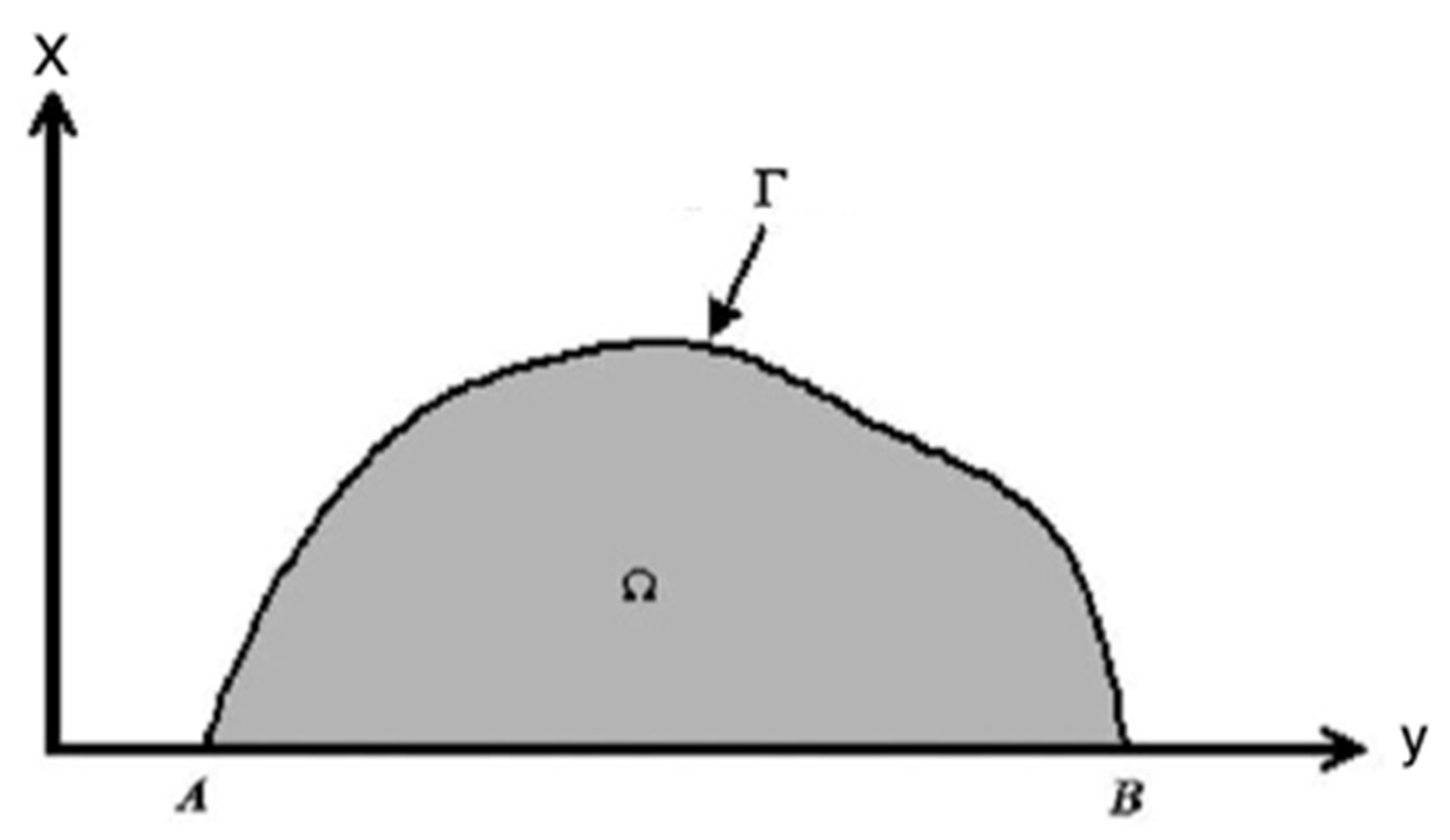
Figure 2.
Variation in the thermal stress sensitivity along the -axis for two different softening parameters of local and nonlocal theories.
Figure 2.
Variation in the thermal stress sensitivity along the -axis for two different softening parameters of local and nonlocal theories.
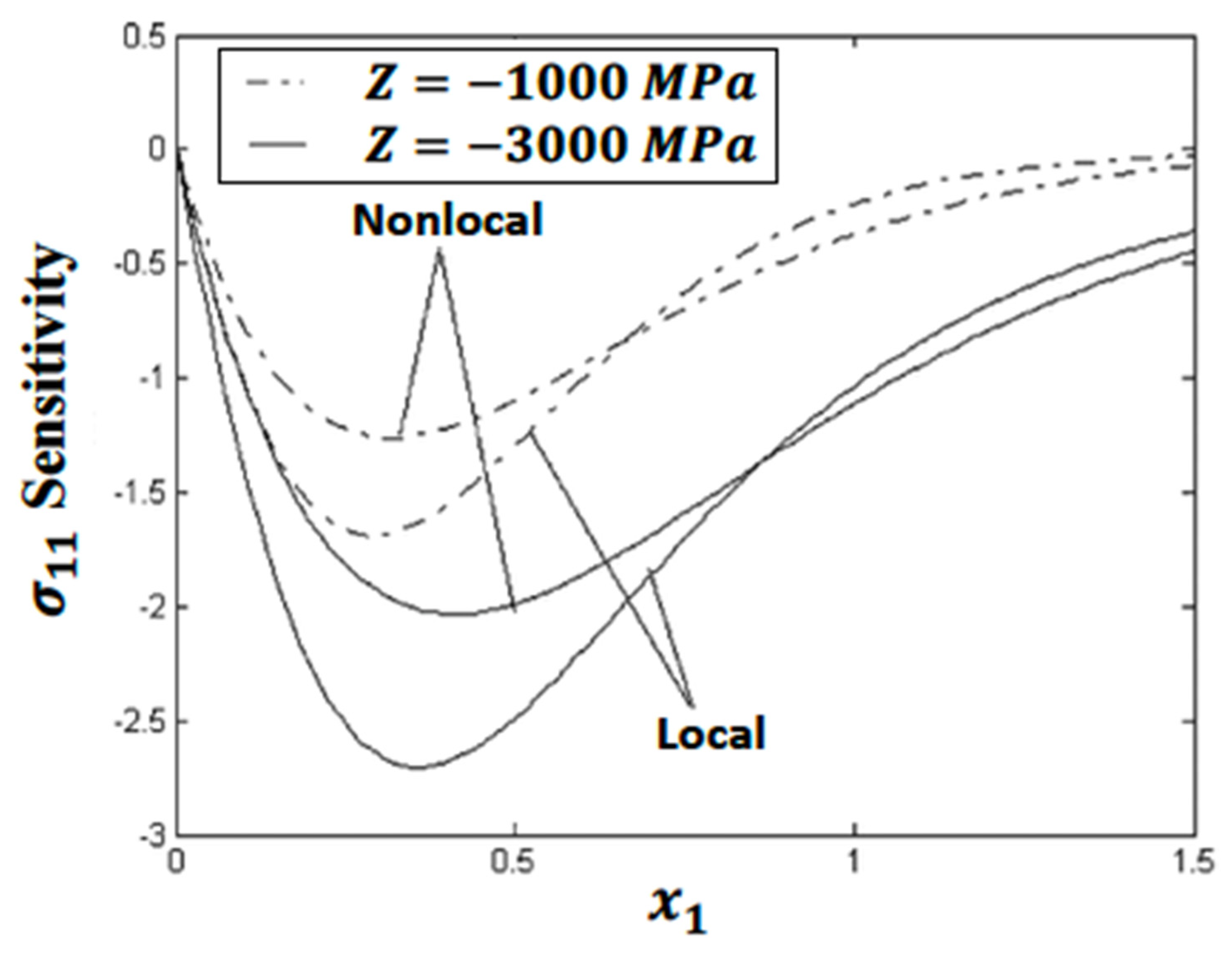
Figure 3.
Variation in the thermal stress sensitivity along the -axis for two different softening parameters of local and nonlocal theories.
Figure 3.
Variation in the thermal stress sensitivity along the -axis for two different softening parameters of local and nonlocal theories.

Figure 4.
Variation in the thermal stress sensitivity along the -axis for two different softening parameters of local and nonlocal theories.
Figure 4.
Variation in the thermal stress sensitivity along the -axis for two different softening parameters of local and nonlocal theories.

Figure 5.
Variation in the thermal stress with time for different methods.
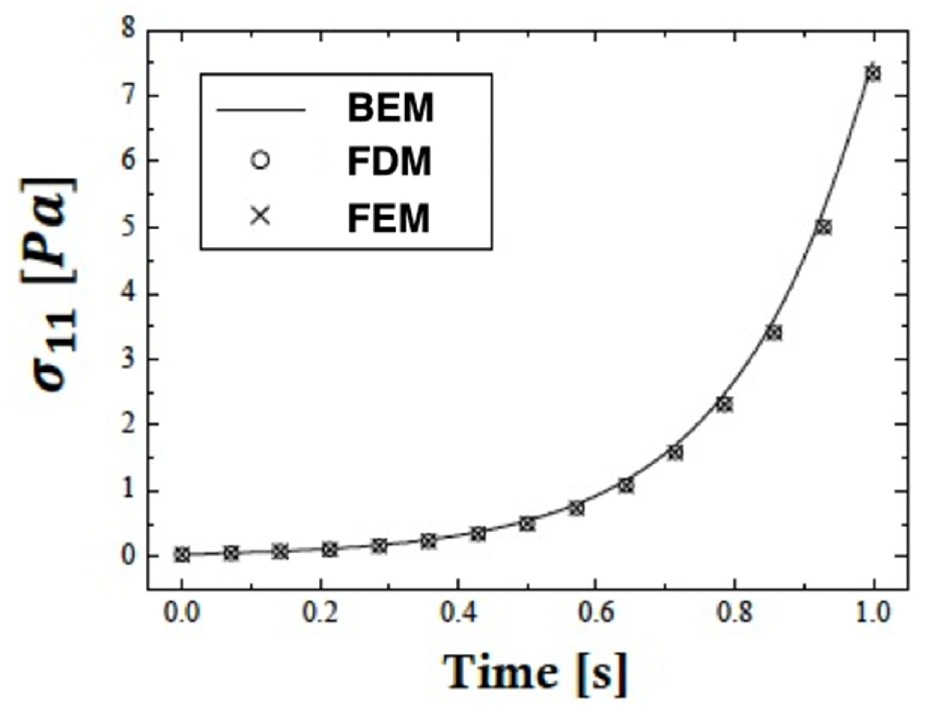
Figure 6.
Variation in the thermal stress with time for different methods.
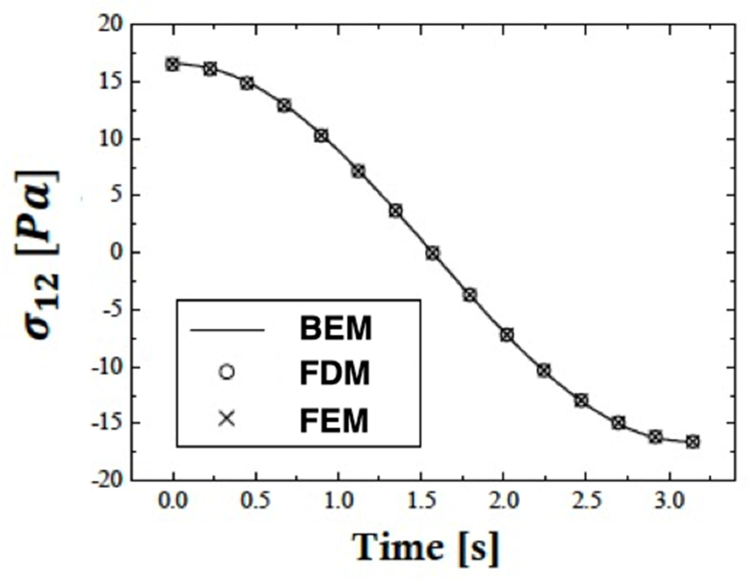
Figure 7.
Variation in the thermal stress with time for different methods.


Table 1.
Numerical results for the considered iteration methods.
| Method | Iter. | CPU Time | Rr | Err. | |
|---|---|---|---|---|---|
| SCAS-GMRES | 40 | 0.0123 | 1.84e−07 | 1.62e−09 | |
| FMDTS | 70 | 0.0567 | 6.62e−07 | 1.84e−07 | |
| UC-RSCSCS | 80 | 0.0795 | 8.42e−07 | 2.56e−06 | |
| SCAS-GMRES | 50 | 0.0594 | 0.16e−06 | 2.12e−08 | |
| FMDTS | 100 | 0.2278 | 1.68e−05 | 4.25e−06 | |
| UC-RSCSCS | 140 | 0.3784 | 1.09e−04 | 0.48e−05 | |
| SCAS-GMRES | 60 | 0.1768 | 2.45e−05 | 1.74e−07 | |
| FMDTS | 280 | 0.7948 | 1.76e−04 | 3.82e−05 | |
| UC-RSCSCS | 300 | 0.8964 | 1.34e−03 | 4.54e−04 |
Table 2.
A comparison of the computer resources required to model stress sensitivity of nonlocal thermo-elasto-plastic damage problems.
Table 2.
A comparison of the computer resources required to model stress sensitivity of nonlocal thermo-elasto-plastic damage problems.
| BEM | FDM | FEM | |
|---|---|---|---|
| Number of nodes | 50 | 50,000 | 45,000 |
| Number of elements | 25 | 15,000 | 13,000 |
| CPU time [min.] | 3 | 150 | 130 |
| Memory [Mbyte] | 1 | 130 | 110 |
| Disc space [Mbyte] | 0 | 190 | 170 |
| Accuracy of results [%] | 1.0 | 2.6 | 2.4 |
Disclaimer/Publisher’s Note: The statements, opinions and data contained in all publications are solely those of the individual author(s) and contributor(s) and not of MDPI and/or the editor(s). MDPI and/or the editor(s) disclaim responsibility for any injury to people or property resulting from any ideas, methods, instructions or products referred to in the content. |
© 2024 by the author. Licensee MDPI, Basel, Switzerland. This article is an open access article distributed under the terms and conditions of the Creative Commons Attribution (CC BY) license (https://creativecommons.org/licenses/by/4.0/).
Share and Cite
MDPI and ACS Style
Fahmy, M.A. BEM Modeling for Stress Sensitivity of Nonlocal Thermo-Elasto-Plastic Damage Problems. Computation 2024, 12, 87. https://doi.org/10.3390/computation12050087
AMA Style
Fahmy MA. BEM Modeling for Stress Sensitivity of Nonlocal Thermo-Elasto-Plastic Damage Problems. Computation. 2024; 12(5):87. https://doi.org/10.3390/computation12050087
Chicago/Turabian StyleFahmy, Mohamed Abdelsabour. 2024. "BEM Modeling for Stress Sensitivity of Nonlocal Thermo-Elasto-Plastic Damage Problems" Computation 12, no. 5: 87. https://doi.org/10.3390/computation12050087
Note that from the first issue of 2016, this journal uses article numbers instead of page numbers. See further details here.