
Manufacture of Microstructured Optical Fibers: Problem of Optimal Control of Silica Capillary Drawing Process


1
Applied Mathematics Department, Perm National Research Polytechnic University, Komsomolsky Avenue 29, 614990 Perm, Russia
2
Perm Federal Research Center, Ural Branch, Russian Academy of Sciences, 13a Lenin Street, 614990 Perm, Russia
*
Author to whom correspondence should be addressed.
Computation 2024, 12(5), 86; https://doi.org/10.3390/computation12050086
Submission received: 11 March 2024
/
Revised: 19 April 2024
/
Accepted: 20 April 2024
/
Published: 23 April 2024
(This article belongs to the Special Issue Mathematical Modeling and Study of Nonlinear Dynamic Processes)
Abstract
:The effective control of any technological process is essential in ensuring high-quality finished products. This is particularly true in manufacturing knowledge-intensive and high-tech products, including microstructured photonic crystal fibers (PCF). This paper addresses the issues of stabilizing the optimal control of the silica capillary drawing process. The silica capillaries are the main components of PCF. A modified mathematical model proposed by the authors is used as the basic model of capillary drawing. The uniqueness of this model is that it takes into account the main forces acting during drawing (gravity, inertia, viscosity, surface tension, pressure inside the drawn capillary), as well as all types of heat transfer (heat conduction, convection, radiation). In the first stage, the system of partial differential equations describing heat and mass transfer was linearized. Then, the problem of the optimal control of the drawing process was formulated, and optimization systems for the isothermal and non-isothermal cases were obtained. In the isothermal case, optimal adjustments of the drawing speed were obtained for different objective functionals. Thus, the proposed approach allows for the constant monitoring and adjustment of the observed state parameters (for example, the outer radius of the capillary). This is possible due to the optimal control of the drawing speed to obtain high-quality preforms. The ability to control and promptly eliminate geometric defects in the capillary was confirmed by the analysis of the numerical calculations, according to which even 15% deviations in the outer radius of the capillary during the drawing process can be reduced to 4–5% by controlling only the capillary drawing speed.
1. Introduction
Fiber optics has been one of the most promising and rapidly developing high-tech industries for the last couple of decades [1,2,3]. This is due to the ever-increasing application of fiber optic technologies in various sectors of the economy: communications [4,5], navigation [6], medicine [7], new materials [8,9], fiber sensorics [10,11,12,13], etc. [14,15]. Instrument engineering is very indicative in this regard, as fiber optics has caused a true revolution, resulting in a generation of instruments and devices based on new physical principles [16,17,18,19,20,21]. As mentioned above, the manufacture of optical fibers is a rather expensive and complex process [18]. Therefore, despite the extensive research on fiber optics, many unsolved problems remain. In our opinion, there are two main reasons for such a situation: first, the lack of study of many issues and, therefore, the lack of information; second, the fact that the practical implementation of modern technologies is often performed ahead of full scientific description and research. All of the above applies fully to the problem of control, including the optimal control of the silica capillary drawing processes for microstructured optical fibers. These are often referred to as photonic crystal fibers (PCF), hollow fibers or holey fibers [22,23,24]. They are used in optical telecommunications [25], optical metrology [26], sensorics [27] and other fields.
There are two fundamentally different technologies for PCF manufacture. The first of them, called “stack and draw”, consists of lining the core with several layers of thin glass capillaries, each of which typically has a round or six-sided cross-section [28]. The second manufacturing method is based on the multiple drilling of parallel holes in a solid cylindrical silica preform [29]. The main quality criterion during the drawing stage is the preservation of all geometric proportions and cross-sectional shapes of the preform and the fiber.
The industrial manufacture of capillaries or glass tubes for PCF (for the “stack and draw” process) is achieved by one of the known methods, such as the Danner process or the Vello process (Danner and Vello), as well as drawing tubes vertically up or down [30,31,32]. All these processes involve drawing an “infinitely long” glass tube from the melt, from which pieces longer than 1 m are cut off. The Danner process is a horizontal drawing process, the Vello process is a vertical drawing process with deflection, and the drawing process is the Vello process but without deflection. The main optical and mechanical properties of silica fibers depend on many factors [31]. The first is the quality of the initial preform. Here, the evaluation of its taper and the presence of small internal defects and bonds play an important role. However, equally important factors are the chosen technological modes of the manufacturing process. Critical among them is the so-called drawing ratio (the correlation of the fiber drawing speed and the silica preform feeding speed), as well as the parameters of the furnace that heats the preform [33]. An important aspect of the drawing manufacturing process is the shape control of the drawn tube [34]. There are several modeling approaches to estimate the capillary shape. For axisymmetric tubes, models for the calculation of the tube cross-sectional area and capillary wall thickness are well known [35]. The shape of the tube can also be estimated by observing the value constancy of the outer and inner radii of the glass tube [36,37]. Previous works show that the constancy of the geometrical characteristics of the tubes is influenced by the drawing speed, the pressure inside the tube, the temperature of the furnace and the silica melt. However, it is the drawing speed that has a significant effect on the shape variation of the cylindrical tube [38]. Therefore, the drawing speed is used as a control action to achieve constant geometric characteristics in tubes in several works [35,38,39].
The problem of drawing a whole silica fiber was studied in [40], but, here, the profile formation of the drawn fiber was carried out based on the balance of the surface forces and agreement with experimental data. As shown for a particular drawing machine, there is an upper limit to the drawing speed at which the fiber can be drawn without breaking, and the practical ranges of the drawing speed and furnace temperature are determined to make the drawing process feasible. Results regarding the stability ranges of the process parameters were obtained in [37], where the critical ratios of the drawing process were calculated and a study was conducted concerning the influence of the furnace design on the stability of the drawing. Considering that the drawing speed is mainly chosen as a control parameter in optimization problems, the results obtained in these works can be considered important in the context of this study. In [41,42], the process of whole fiber drawing was also studied, and it also proposed a variational method to calculate the optimal parameters of its drawing process. Note that the process described in these works can be considered as an asymptotic approximation of the case described in this paper. It should be noted that there are significant differences in the formulation of optimization problems for the processes of drawing solid preforms and capillaries. In the first case, the control of the drawing process is reduced to the observation of the geometric shape of the outer surface of the silica cylinder. In the second case, it is important to observe the inner surface to avoid the implosion or inflation of the capillary [34,36]. The issues regarding the optimal control of the silica capillary drawing process in the variational formulation are studied in [35,39]; first-order optimality conditions are obtained, and a gradient method to find the optimal state of the system is proposed.
The control system that exists in practice is usually based on the well-known theory of PID controllers [43]. According to this theory, the outer radius of the tube is constantly monitored during the drawing process. Based on the measurement results, a corresponding control action is generated, which dampens the perturbations (radius deviations). Furthermore, measurements are taken at only one point located far enough from the furnace outlet. Therefore, if the deviations are larger than allowed, a part of the capillary will be substandard.
A slightly different approach is proposed in this paper:
- (1)
- radius deviations are measured in a certain area, i.e., at several points;
- (2)
- the measuring area and the radius control point are spaced along the length of the flow, with the measuring area as close as possible to the furnace outlet;
- (3)
- the control action (change in drawing speed) is determined from the solution of the optimal control problem of the distributed system.
This formulation of the problem allows us to obtain more complete information about the system perturbations and to completely or partially level out the perturbations (measurement and control areas are separated) and also allows the control action to be optimal.
Let us explain the essence of the proposed approach in more detail. The study is based on a nonlinear dynamic model that describes the process of drawing a silica capillary. The model is represented by a system of differential equations of motion, continuity and energy for the functions of the melt velocity, outer and inner radii and capillary temperature. The model takes into account all types of heat exchange with the environment, the influence of inertial forces, etc. By comparing the calculated data with experimental data, the model is checked for its adequacy. Acceptable congruence between these results is shown, which makes it possible to use the proposed model when solving the problem of the optimal stabilizing control of a distributed system. Next, the original system of differential equations is linearized. For a linearized system, the problem of the optimal control of the drawing speed is formulated and solved. One of the variants of the Lagrange method is used, which makes it possible to reduce the optimization problem to solving a boundary value problem. In this case, an explicit representation of the optimal drawing speed as a function of time is obtained. For the numerical implementation of the optimization system, the finite element method of the Comsol Multiphysics package is used. The influence of the effect of optimal stabilizing control on the evolution of the geometric defect of the preform is analyzed.
The overall objective of this work is to systematize and solve the optimal control problem of capillary drawing processes, and, finally, to provide recommendations for the selection of process regimes leading to a stable drawing process.
2. Mathematical Modeling of the Capillary Drawing Process
2.1. General Mathematical Model of Silica Capillary Drawing
Several works [31,32,33] are devoted to the mathematical modeling of capillary drawing technological processes, in which an analysis of the mathematical aspects and features of the models is given, and numerical results are presented. The mathematical model of such a process is described by a system of partial derivative equations, namely the equations of motion, continuity and energy.
It should be noted that the first works in this direction referred to the drawing of continuous fibers, and now there is a wide range of such models that allow us to consider the problems in different formulations and calculate different types of heat transfer [33]. As for the mathematical models of capillary drawing (Figure 1), they were proposed somewhat later, specifically in the early 2000s. At that time, a paper [31] was published presenting a quasi-one-dimensional model of capillary drawing. This model takes into account the effects of the inertial forces, viscous friction forces, surface tension and pressure inside the capillary, as well as all types of heat exchange.
In the proposed work, a modified model of tube drawing is presented. Compared to the above model, it differs in that the radiative heat transfer is considered more strictly. First, it considers that the thermal conductivity of silica is due to two mechanisms: molecular and radiative conductivity [44]:
where is the molecular (conductive) component, is the Stefan–Boltzmann constant, is the refractive index of light, is the Rosseland mean extinction coefficient of the silica and is the temperature of the silica. Second, in deriving the energy equation, the contribution of radiation to the temperature distribution in the capillary is evaluated more rigorously. The Planck, Stefan–Boltzmann and Lambert laws are used for this purpose [45]. It is known that the radiation spectrum of a black body at temperature is determined by Planck’s law:
where c is the speed of light, is the frequency, is the Boltzmann constant and is the Planck constant. For the integral flux density, according to the Stefan–Boltzmann law, we have
Radiant heat exchange between bodies is determined by Lambert’s law: the amount of energy radiated by a surface element dA2 in the direction of element dA1 (Figure 2) is proportional to the energy radiated along the normal EndA2, multiplied by the value of the elementary solid angle and , i.e.,
Real technical materials do not absorb radiation completely. To characterize them, the concept of the degree of blackness () is used, and Planck’s and Stefan–Boltzmann’s laws are applied with this correction coefficient. For example, for the flux density, instead of (3), we use the expression Let us denote by the normal to the point of the silica fiber surface, and by the segment connecting points and (Figure 2). The resulting radiation flux at the surface point is the sum of the flux of its own radiation and the absorbed flux. Consequently, the following relation expresses the law of conservation of energy (in the approach of a black body, ):
Here, the integration is over the area , which is the part of the thermocouple boundary, which is visible from the point . The variable is used to specify the distance along the thermocouple. Then, the distance between the point on the silica and the point on the thermocouple is . Here, is the radius of the thermocouple, and is the outer radius of the cylindrical surface of the silica.
Based on the heat fluxes for the elementary volume bounded by sections , and the surface element dA1, the energy equation is obtained. Then, the system of equations describing the motion and heat exchange during capillary drawing, supplemented with initial and boundary conditions, has the form
where are the velocity of the substance, the inner and outer radii of the capillary and the melt temperature, respectively; x is the longitudinal coordinate, t is the time and L is the length of the drawing area; is the difference between the internal and external pressures, is the specific heat capacity of the melt, is the melt density, is the absorption coefficient of the fiber surface, is the degree of blackness of the heating element, is the degree of blackness of the melt, is the gas temperature inside the tube, is the ambient temperature, is the radiation coefficient from the preform surface outside the furnace, is the surface tension coefficient, is the dynamic viscosity of the melt, , are the heat transfer coefficients from the inner and outer surfaces of the furnace, respectively, is the length of the heating zone, is the furnace temperature and is the weighting coefficient,
The system (6) is supplemented by initial and boundary conditions of the form
Here, is the law of the preform feed rate, is the drawing speed, and , are the functions for the determination of the initial and boundary values of the inner and outer radius of the capillary; is the law of the preform temperature change at and at the initial moment in time.
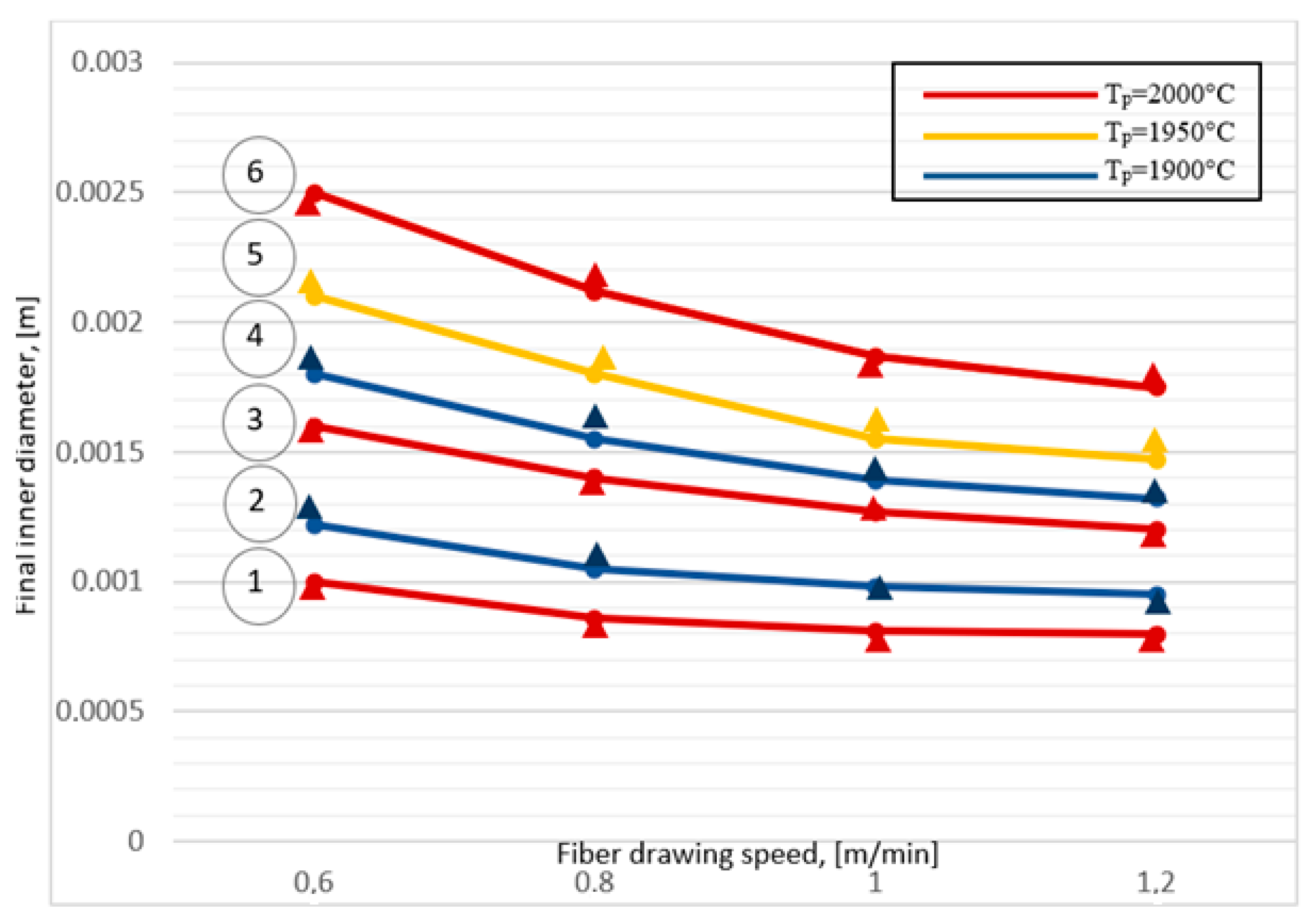
To verify the adequacy of the modified mathematical model (6), the numerical calculations were compared with the experimental data presented in [46]. In the cited work, the results of 24 measurements of the finished product’s radii during capillary drawing were presented. The preform was made of Suprasil F300 glass with an outer radius = 1.4 × 10⁻⁴ m and an inner radius = 1.2 × 10⁻⁴ m. The preform was fed into the furnace at a constant rate and the top of the tube was left open to the atmosphere. The feed rate was varied from 2 × 10⁻³ m/min to 8 × 10⁻³ m/min, and the drawing speed was varied from 0.6 m/min to 1.2 m/min at furnace temperatures Tp in the range of 1900 °C, 1950 °C and 2000 °C. Both the outer and inner diameters were measured during the experiment.
Numerical studies were carried out in the Comsol Multiphysics software, and the results for the inner radius are shown in Figure 3. As can be seen from the figure, the numerical results obtained in this work coincide quite well with the experimental data. A similar pattern was observed for the outer radius.
Thus, the modified model (6) used in this work describes the process of silica tube drawing with sufficiently high accuracy, taking into account the main acting forces and all types of heat transfer occurring inside the furnace. It should be noted that the above model was used by the authors to study the stability of the capillary drawing process [37].
2.2. Mathematical Model of Stabilizing Optimal Control of Silica Capillary Drawing
Let us assume that the physical process of capillary drawing, whose mathematical model is represented by the system (6), is controllable. The typical control action in this process is the drawing speed of the silica capillaries . The control objective is to keep the inner and outer diameter of the silica tube in the scope of a given state. Let the selected control correspond to the functions , , , , which are solutions of the system of Equation (6). Let us call the combination of these five functions the program process of capillary drawing.
In real conditions, the actual distributions of the values , , , will differ from the program distributions of , , , by some deviations (perturbations), which are known to be rather small values compared to the program values. The property of perturbation smallness serves as a basis for the neglect of the products of the perturbations of the sought functions in the process of research. In other words, the analysis of a system linearized at the area of its stationary state can replace the analysis of the original nonlinear system [33,34,37,38,41,47]. There are different means of linearization; here, we use the method described in [38].
Thus, in the first stage, linearization was performed, in which the parameters that determined the state of the system were divided into the main and perturbance parameters , such that
The stationary solutions of the system (6) act as the main parameters. The result is a system describing the evolution of perturbations. To simplify the notation, we use .
Considering this remark, the linearized system of Equations (6) takes the form
The coefficients in (8) have the form
where is the right part of the continuity equations in (6), calculated for the stationary state drawing mode; is the viscosity in the stationary state drawing mode, is the kinematic viscosity and .
3. Optimal Control of the Capillary Drawing Process
3.1. Isothermal Case
Let us first address the problem of controlling the capillary drawing process under isothermal conditions. The general mathematical model described in Section 2 has the following form in the isothermal case:
The model (9) is supplemented with initial and boundary conditions of the form
The model (9), (10) is a one-dimensional nonstationary isothermal model in the form of an initial boundary value problem with a differential operator of the parabolic type. It is important to note that the actual capillary production process for PCF is of very high precision. This is due to the fact that the geometric dimensions of the silica undergo multiple changes during the drawing process. The same colossal differences can be observed in the changes in the velocity and viscosity regimes. This requires the highly precise adjustment of the drawing tower, precise program support and the skill of the process control engineer. The slightest adjustments to the program values of the control parameters can lead to the complete destabilization of the process. However, such corrections are necessary and it is important to quickly and correctly calculate the measure of the control actions on the system. This need may arise, for example, in the case of a geometric defect in the preform. This may be a top material lack due to the presence of an air bubble in the silica at the preform manufacturing stage, or the global violation of the cylindricity of the preform, manifested in its taper or the presence of bonds (Figure 4).
Since isothermal drawing is a special case of the process described in Section 2, the linearization of the isothermal model is a trivial task. As before, the stationary state is chosen as the initial (program) state of the system. The model describing the evolution of small perturbations , is written in the form
The initial and boundary conditions take the form
Here, the functions in the numerators of the fractions are the actual values of the radii and velocities. The denominators contain the program stationary values. Therefore, if the actual values exactly match the program values, we have a differential problem with homogeneous initial and boundary conditions, which have a single zero solution. In practice, this would mean the complete absence of deviations in the silica capillary geometries and particle transport velocity from the reference values. However, this is often not the case in real manufacturing conditions. We further assume that one of the initial or boundary conditions in (12) is not zero, while the other conditions are zero. For example, suppose that a defect has the outer radius of the preform and that this defect is described by the condition
In order to eliminate the defect, we select the drawing speed as the control function:
The objective of the control in this case is to stabilize the geometric shape of the drawn tube, i.e., to eliminate the defect on the finished capillary. It is standard procedure in the silica tube manufacturing process to control the geometric shape of the finished product. The drawing tower usually includes a laser scanner to perform such control, which is usually installed near the outlet area of the finished product. Let us describe the objective of the optimal control problem with an integral type functional.
Thus, the optimal stabilization control problem (11)–(15) is formulated. This includes a boundary trade-off control problem and a boundary monitoring problem [48]. We will not investigate the existence of a solution to the minimization problem (11)–(15) in this paper. Note that the study of the existence of a solution to the minimization problem is reduced to the proof of semi-continuity from below and the coercivity and convexity of the objective functional and has been carried out by the authors in earlier papers [41]. It is also known that since the real capillary wall dimensions are counted in fractions of a millimeter, a defect in the outer radius will certainly have a negative effect on the formation of the inner radius profile. In a real manufacturing process, the scanner cannot monitor the geometry of the hidden inner radius. Therefore, it may be appropriate to monitor the values of both the outer and inner radii using a constructed mathematical model, trying to minimize all possible defects at the same time:
If the problem of controlling the constancy of the geometric properties of the inner wall of the capillary is not necessary, we can limit ourselves, as suggested earlier, to the objective function of the form (15). Here, is the control time, and is the regularization parameter, known in the literature as the “control cost” [48]. Thus, the differential problem (11), (12), supplemented with conditions (13), (14) describing the defect of the preform geometry and the type of control action on the system, as well as one of the objective functionals (15) or (16), form a general formulation of the problem of the optimal control of capillary drawing for PCF production.
Let us obtain the necessary optimality conditions for the formulated minimization problem. The necessary optimality conditions are obtained in the form of an initial boundary value problem for the components of the state vector (consisting of three components) and their dual states (functions ). By imposing several constraints on the region of admissible control, it becomes possible to pass from the variational inequality to the variational equality [26], where is the minimizer, is the Gato differentiation operator and is the element variation of . Thus, the optimality conditions follow in the form of the so-called optimization system. Furthermore, it becomes possible to obtain the analytical dependence of the optimal control function on the dual radii and the velocity. By omitting several technical transformations similar to those performed in [41,42,47] for the case of a solid (incomplete) preform, we obtain the general form of the optimality system. Thus, for the objective functional (15), the optimality system has the form
The optimal control function satisfies the relation
The optimization system is a boundary value problem consisting of six partial differential equations, some of which are given conditions at the initial time (initial conditions), and the rest are given conditions at the final time . Such inconsistency in the system equations in time is a distinctive feature of the optimization systems for problems in such formulations. Optimality conditions (17) in the form of a differential problem are convenient to use because, in this case, the optimal control function is determined from its solution by the explicit law (18).
The optimality system for the problem with the objective functional (16) has the form
The optimal control function in this case satisfies the relation
3.2. Non-Isothermal Case
To describe the flow of a silica melt in the non-isothermal case, let us return to the modified quasi-one-dimensional mathematical model of silica capillary drawing (6), (7), which takes into account all types of heat exchange: heat conduction, convective heat exchange with the environment and radiation. The full justification of the model is given in Section 2 of this paper.
The problem of the optimal control of the drawing process is formulated (as in the isothermal case) in the language of small perturbations. The model (6), (7) is linearized in the area of its stationary state. Of interest for the observation is the development of small possible perturbations in the linearized model in the form of inhomogeneities in the initial and/or boundary conditions. To control the stabilization process, it is proposed to vary the small deviations in the drawing speed. The control objective is to balance the effects of small perturbations in the observable region of the problem solution.
A linearized model and formulation of the optimal stabilization control problem with boundary control (drawing speed) and boundary observation (of the shape of the outer surface of the finished fiber) is presented:
The objective function has the form:
The relation (22) determines the smallness of the deviations in the outer radius of the capillary in the draw control zone at . The problem is posed as a trade-off control problem, and is the control cost. Here, is the function defining the geometry of the preform surface defect, and is the control function (capillary drawing speed).
For the linear control problem, similarly to Section 3.1, we obtain the necessary optimality conditions in the form of a boundary differential problem for the deviation functions of the actual values from the program values, and states conjugated to these deviations are obtained. The optimization system of the control problem (21), (22) has the form
As in the isothermal case, the equations of the system (23) have several peculiarities. One of them is a different course of the variable “time”, which causes certain difficulties in the realization of its solution. However, the weak coupling of the blocks of equations (only through the boundary conditions for the functions and at the point x = L) allows us to use special iterative methods to find solutions quickly. An undoubted advantage of this approach is the existence of an explicit expression of the values of the optimal control function. Thus, if the solution (23) is known, in particular, if the functions of the conjugate states are found, it is possible to adjust the drawing speed according to the following law:
4. Results and Discussion
Let us present the results of the numerical calculations of optimization systems for the isothermal case. The numerical implementation was carried out using the finite element method. The program was implemented in Comsol Multiphysics. Special attention was paid to the fact that some of the equations of the optimization system have a direct solution in the “time” coordinate, and some of the equations are solved with a backward solution in this coordinate. The time inconsistency of the system equations caused certain difficulties in the joint solution of the equations. To overcome them, additional iterative methods were used.
Thus, it is evident that in (17), (19) and (23), the equations for perturbations of the radii, speed and temperature are supplemented with initial conditions—that is, conditions at time t = 0. However, for the functions of conjugate states, conditions are specified at the final moment of time t = τ. The scenario for the solution of the optimality system in Comsol Multiphysics implied the creation of six (eight) independent physical PDE blocks. The first three (four) of them were solved together forward in time, with the resulting values transferred to the remaining equations. A negative step was assigned to the “time” variable, and the calculation was carried out from t = τ to t = 0. The resulting values of the conjugate states were again transferred to the first blocks of equations, solved forward in time and so on until the solution process converged.
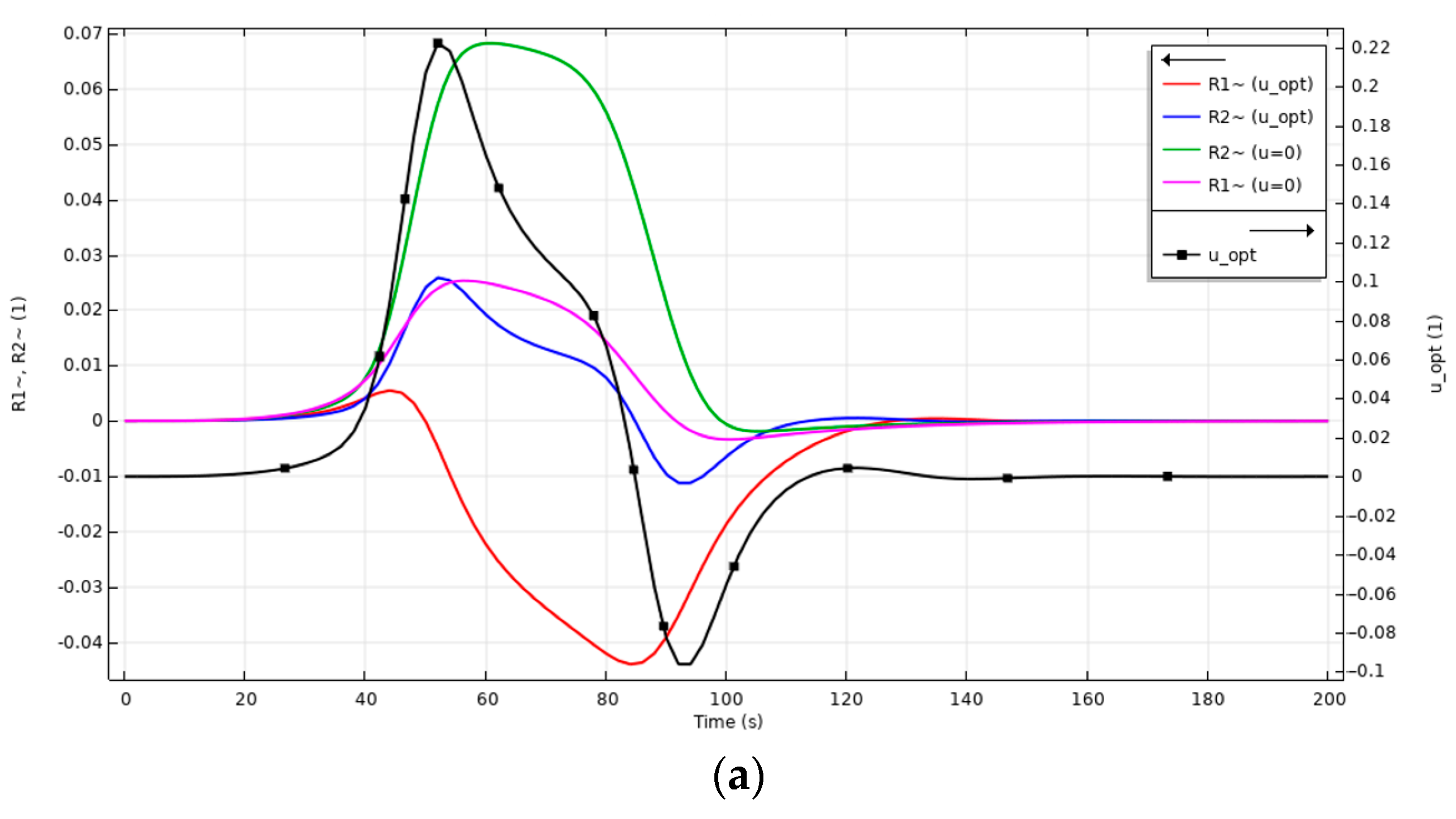
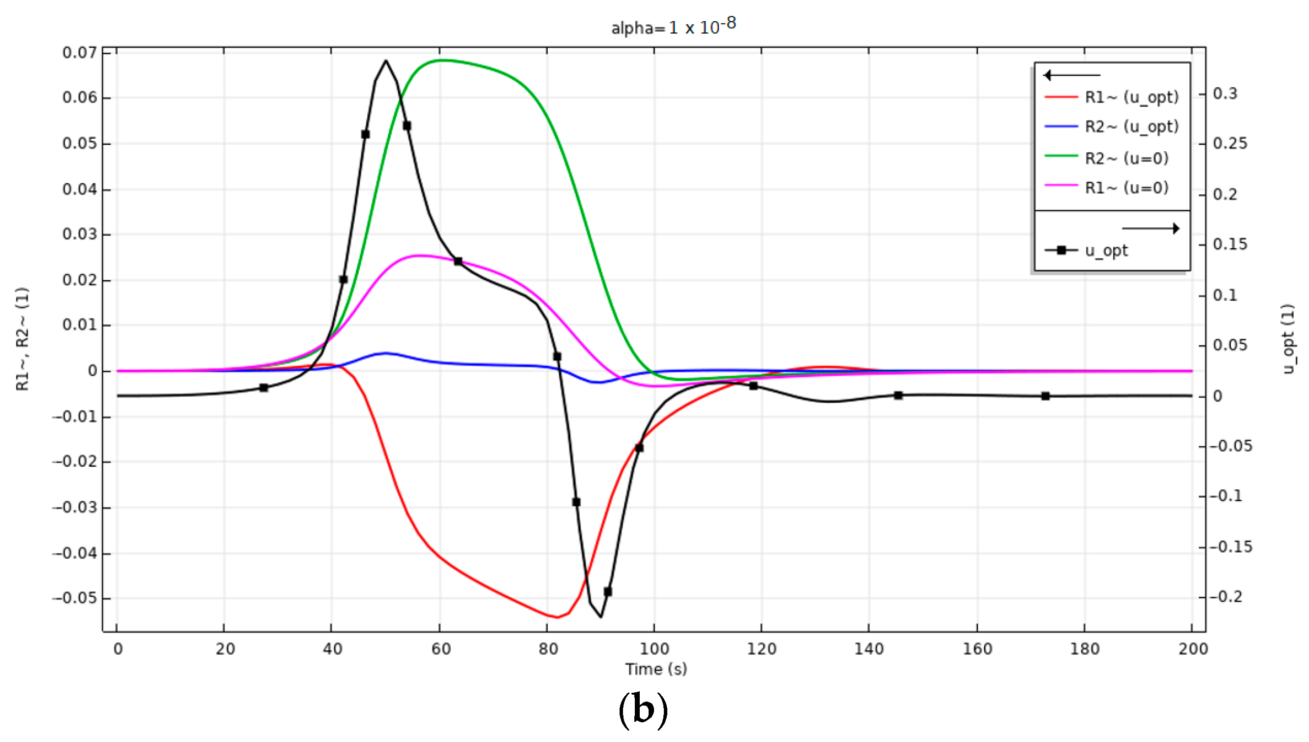
The results of the numerical simulation for the objective functional (15) are shown in Figure 5.
Calculations were performed for a defect value of 5% in the geometric shape of the preform (function ). This choice of defect value is justified by the fact that this value is critical for manufacture and that preforms with defects exceeding this value are usually rejected. The figure shows the deflection profiles of the outer and inner radii at the observation point , i.e., at the elongated capillary. It is shown (Figure 5a) that the deviations from the program value in the uncontrolled drawing mode are about 7% and 2% (green and purple color, respectively). The propagation of the defect towards the inside of the capillary and its very noticeable effect on the inner surface of the capillary are evident. In the controlled mode, the same initial defect can be significantly transformed if the drawing speed is adjusted according to the law (17). In this case, we reduce the value of the defect on the outer surface of the capillary from 7% to 1.5% on average. Of course, the transformation affects the inner surface of the capillary as well. The model calculation shows that the almost complete suppression of the “bulge” defect on the outer wall leads to a slight “retraction” effect on the inner wall (blue and red colors). The law of drawing speed adjustment (black color) is also shown. According to this, during the first 120 s of the process after defect detection, a smooth transition is required to increase the program speed mode by 20%, to then decrease it by 10% and finally to lead it to a smooth transition to a zero value between 100 s and 120 s, which will result in defect suppression. Figure 5b shows the evolution of the deviation profiles of the outer and inner radii of the capillary and at a different value of the control cost parameter. It can be seen that it is possible to almost completely neutralize the defect of the outer radius (blue vs. green), but, since there is no simultaneous control of the inner radius as well, the retraction of the inner wall is quite significant (red). The adjustment of the control in this case ranges from −5.5% to 7%. Thus, the influence of the parameter is quite significant. Here, we also present an analysis of the influence of the values of the regularization parameter on the general picture of the suppression of the capillary geometry defect (Figure 6).
The calculation shows that the effective values of the regularization parameter for this model are from 5 × 10⁻⁹ to 1 × 10⁻⁶. It is shown that increasing the values of to values exceeding 1 × 10⁻⁶ is equivalent to the absence of control. Reducing the values below the level of 5 × 10⁻⁹ is also inefficient since the solutions obtained in this case are infinitely close to each other (yellow and purple color). The compromise option in this calculation is values close to 1 × 10⁻⁷. The results calculated exactly for this value of are shown in Figure 5. In this case, it is possible to significantly reduce the defect on the outer wall of the capillary, while obtaining a less significant “retraction” effect on the inner wall.
The results of the numerical modeling of the optimality system (19) for the objective functional (16) are shown in Figure 7. It shows the evolution of the deviation profiles of the outer and inner radii of the capillary and in the observation zone x = L (elongated capillary). For comparison, two cases are calculated: the result without control (green and purple color) with a 5% defect on the outer surface of the preform and the result with control (blue and red color) with the same defect present. Note that the objective functional (16) in this calculation has the effect of controlling both the outer and inner radii of the capillary. It can be seen that a 7% defect at the outer radius can be suppressed at least three times (blue color vs. green). However, with this suppression, the inner radius is particularly sensitive—there is a tendency for the inner capillary wall to retract (red color vs. purple). Nevertheless, the control result is effective—deviations in the geometry remain but are within the tolerance of 5%. The black color in the same figure shows the profile of the optimal control function—the time correction of the programmed fiber drawing speed. Thus, the results of the numerical studies confirm the possibility of suppressing the existing defects in the preform, while carrying out calculations for different objective functionals allows us to understand this problem at a qualitative level.
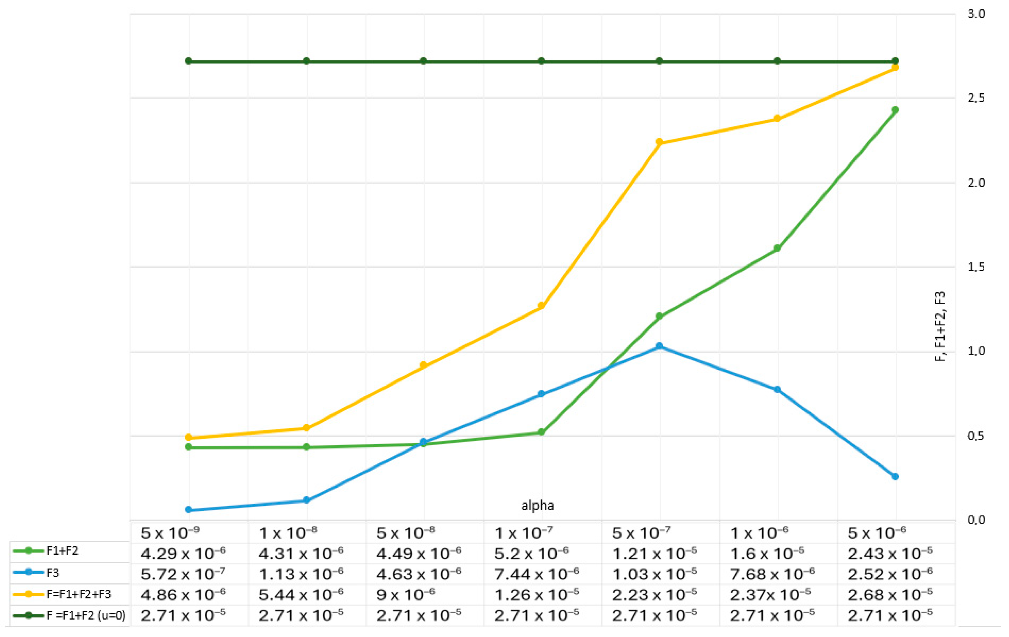
Additionally, for the problem with the objective functional (16), the values of the minimizable functional F and its constituent summands depending on the regularization parameter were evaluated. Let F1, F2, F3 be the first, second and third components of the sum in (16). Figure 8 shows the dependence of the values of these components on the regularization parameter. Calculations show that for values of such as 5.00 × 10⁻⁹–5.00 × 10⁻⁸, the values of the objective functional and all of its components are minimal, which corresponds to capillary drawing in the optimal control mode.
Further, we provide the values of the parameters adopted in the model: the length of the studied section of the drawing, L, [m]—0.5; the inner radius of the preform, , [m]—0.007; the outer radius of the preform, , [m]—0.01; the silica density, [kg/(m3)]—2200; the silica preform feed rate, , [m/s]—5 × 10−4; the drawing speed, , [m/s]—0.1; the free fall acceleration, g, [m/s2]—9.8; the specific heat capacity of the melt, cp, [J/(kg⋅K)]—1500; the typical temperature, T0, [K]—2000; the pressure difference acting on the inner and outer surfaces of the capillary, p0, [Pa]—0; the kinematic viscosity, , [m2/s]—17.871; and the control time, , [s]—200.
5. Model Verification Proposal
Any analytical model or proposed method requires experimental verification. The simulation results obtained in this study are no exception. However, such a complex process as the fabrication of microstructured optical fibers is not available to every university laboratory. In addition, part of the verification process is the lengthy acquisition of statistical data, which makes the process of checking the model’s adequacy quite expensive. In this section of the paper, we give several suggestions for the possible verification of the model in the conditions of real optical fiber production and optical research laboratories.
The first crucial stage of the verification process is the meticulous implementation of technological operations, adhering to all recommendations for process control outlined in this work. It is of paramount importance to ensure that the production area is kept clean [49], that all safety precautions are in place and that the operating instructions for the drawing tower and all additional equipment are followed.
The second stage is to assess the variation in the optical–geometric parameters of the fiber along its length. At the early stages, it is necessary to evaluate the geometric parameters of the fiber by dividing it into separate fragments and studying all the fiber tips (cross-sections) under a microscope. After the basic geometric parameters begin to vary from section to section, i.e., the number and location of capillaries is observed, it is advisable to resort to non-destructive research, which is widely practiced for other types of fibers [50,51,52,53]. The optimal way to study these types of samples is optical frequency domain reflectometry (OFDR) [54,55,56,57]. This approach is based on the injection of continuous frequency-scanning high-coherence optical radiation into the fiber under study and the interference of its backscattered part with the same probing signal. Due to the fact that the typical optical signal attenuation coefficients in microstructured fibers are quite high [58], the OFDR method seems to be quite convenient, since continuous radiation allows one to obtain a clearly visible backscattering pattern. Another important advantage of the method is the ability to select the frequency scanning range, which makes it possible to adjust to the operating wavelengths of the fiber under test. The proof of the suitability of the method for the study of the characteristics of microstructured fibers is the widespread use of these fibers as the sensor elements of OFDR-based systems [59,60]. When studying short lengths of optical fibers, it is advisable to exploit the possibility of measurement with an ultra-high resolution, which is fundamentally limited in the region of several tens of microns; when studying long fragments obtained immediately after drawing from the preform, it is advisable to use settings that provide measurements with a coarser resolution. In the case of measuring optical fibers with an extremely high optical attenuation coefficient, the use of two-stage erbium amplification in the OFDR circuit is recommended [61]. Of no small importance for microstructured fibers are the parameters of the evolution of the radiation polarization state along their length. Most optical frequency domain reflectometers are equipped with two detectors that detect two states of polarization [62]. Studying the backscattered power for each polarization state will provide basic information about the anisotropy properties of the fiber, as well as its modal birefringence, as occurs with different anisotropic fibers [63,64].
In the general case, applicable for many types of microstructured fibers, the main criterion for the optimal control of the drawing process will be the constancy of the attenuation coefficient of the optical signal at the operating wavelength along the length of the fiber. The signal from an optical frequency domain reflectometer is quite heavily distorted by noise, so it is necessary to apply special processing methods. Our practice has shown that the elimination of noise of this kind is optimally implemented using the activation function dynamic averaging and frequency domain dynamic averaging methods, which give good results in both the time and frequency domains [65]. These measures will help to increase the signal-to-noise ratio by 10 dB; thus, the OFDR trace will become a smooth line along which it will be possible to evaluate the uniformity of the attenuation coefficient and/or the evolution of the polarization state of the radiation. We hope that this brief methodology will allow one to verify the data in this work in industrial production conditions.
6. Conclusions
This paper studies the issue of the optimal control of silica capillary drawing processes. The study is based on a nonlinear mathematical model of the nonstationary process of silica tube drawing based on the equations of continuity, motion and energy. The proposed mathematical model is tested for its adequacy. Optimal control problems are formulated for a linearized system of differential equations in the area of a particular state. The objective functions in these formulations have the purpose of minimizing geometric defects on the capillary. Using a generalization of the Lagrange principle, necessary optimality conditions are obtained in the form of boundary value problems for the melt velocity, outer and inner radii of the capillary and silica temperature, as well as four functions of conjugate states. Numerical results are obtained in the isothermal case, and the cases of controlling the constancy of only the outer radius and the outer and inner radii of the capillary are studied. The speed of the drawing process is chosen as the control. The influence of the regularization parameter on the magnitude of the control actions and, as a consequence, on the possibility of suppressing the existing geometrical surface defect is also studied. In addition, an approach to the experimental verification of the mathematical model of the optimal control of the drawing process is proposed. This approach is based on optical reflectometry of the frequency range of the finished optical fibers. Note that the method developed by the authors differs significantly from the currently widely used approach based on PID controllers. The advantage of the proposed method is the ability to control and promptly eliminate geometric defects in the capillary. This is confirmed by the analysis of the above numerical calculations, according to which even 15% deviations in the outer radius of the capillary during the drawing process can be reduced to 4–5% by controlling only the capillary drawing speed.
Author Contributions
Funding
The work in Section 5 was carried out within the framework of State Assignment No. 124020600009-2.
Data Availability Statement
The experimental data presented in this study are available upon reasonable request from the corresponding author.
Conflicts of Interest
The authors declare no conflicts of interest.
References
- Agrell, E.; Karlsson, M.; Chraplyvy, A.R.; Richardson, D.J.; Krummrich, P.M.; Winzer, P.; Roberts, K.; Fischer, J.K.; Savory, S.J.; Eggleton, B.J.; et al. Roadmap of optical communications. J. Opt. 2016, 18, 063002. [Google Scholar] [CrossRef]
- Liang, X.; Jiao, K.; Wang, X.; Wang, Y.; Wang, Y.; Bai, S.; Wang, R.; Zhao, Z.; Wang, X. Progresses of Mid-Infrared Glass Fiber for Laser Power Delivery. Photonics 2024, 11, 19. [Google Scholar] [CrossRef]
- Hartog, A.; Liokumovich, L.; Ushakov, N.; Kotov, O.; Dean, T.; Cuny, T.; Constantinou, A.; Englich, F. The use of multi-frequency acquisition to significantly improve the quality of fibre-optic-distributed vibration sensing. Geophys. Prospect. 2017, 66, 192–202. [Google Scholar] [CrossRef]
- Varshney, A.; Goya, V. Fiber Optics Communication: Evolution of Guided Media. Int. J. Res. Appl. Sci. Eng. Technol. (IJRASET) 2024, 12, 2321–9653. [Google Scholar] [CrossRef]
- Gorlov, N.I.; Bogachkov, I.V. The Principles of Information Safety for Physical Channels of Optical Access Networks. Instrum. Exp. Tech. 2020, 63, 591–594. [Google Scholar] [CrossRef]
- Zhang, Y.; Wang, Z.; Wang, G.; Yu, F.; Zhang, B.; Yang, F. Polarization Stability of Spun Fiber Resonator for Resonant Fiber Optic Gyro. IEEE Sens. J. 2023, 23, 15644–15651. [Google Scholar] [CrossRef]
- Mizeva, I.A.; Potapova, E.V.; Dremin, V.V.; Zherebtsov, E.A.; Mezentsev, M.A.; Shuleptsov, V.V.; Dunaev, A.V. Optical probe pressure effects on cutaneous blood flow. Clin. Hemorheol. Microcirc. 2019, 72, 259–267. [Google Scholar] [CrossRef]
- Chung, D.D.L. A Review of Self-Sensing in Carbon Fiber Structural Composite Materials. World Sci. Annu. Rev. Funct. Mater. 2023, 1, 2230004. [Google Scholar] [CrossRef]
- Matveenko, V.; Serovaev, G. Distributed Strain Measurements Based on Rayleigh Scattering in the Presence of Fiber Bragg Gratings in an Optical Fiber. Photonics 2023, 10, 868. [Google Scholar] [CrossRef]
- Chernutsky, A.O.; Khan, R.I.; Gritsenko, T.V.; Koshelev, K.I.; Zhirnov, A.A.; Pnev, A.B. Active Thermostatting of the Reference Optical Fiber Section Method in a Distributed Fiber-Optical Temperature Sensor. Instrum. Exp. Tech. 2023, 66, 824–831. [Google Scholar] [CrossRef]
- Bogachkov, I.V.; Gorlov, N.I.; Monastyrskaya, T.I. Types and Applications of Fiber-Optic Sensors Based on the Mandelstam—Brillouin Scattering Principle. In Proceedings of the 2022 International Conference on Information, Control, and Communication Technologies (ICCT), Astrakhan, Russia, 3–7 October 2022; pp. 1–4. [Google Scholar] [CrossRef]
- Gritsenko, T.V.; Dyakova, N.V.; Zhirnov, A.A.; Stepanov, K.V.; Khan, R.I.; Koshelev, K.I.; Pnev, A.B.; Karasik, V.E. Study of Sensitivity Distribution Along the Contour of a Fiber-Optic Sensor Based on a Sagnac Interferometer. Instrum. Exp. Tech. 2023, 66, 788–794. [Google Scholar] [CrossRef]
- López-Mercado, C.; Itrin, P.; Korobko, D.A.; Zolotovskii, I.O.; Fotiadi, A.A. Brillouin optical time domain analysis with dual-frequency self-injection locked DFB laser. In Proceedings of the Proc. SPIE 12139, Optical Sensing and Detection VII, 121391D, Strasbourg, France, 17 May 2022. [Google Scholar] [CrossRef]
- Ferreira, M.F.S. Optical Fibers: Technology, Communications and Recent Advances; Nova Science Publishers: Hauppauge, NY, USA, 2017; ISBN 9781536109917. [Google Scholar]
- Kharakhordin, A.; Rybaltovsky, A.; Popov, S.; Ryakhovskiy, D.; Afanasiev, F.; Alyshev, S.; Khegai, A.; Melkumov, M.; Firstova, E.; Chamorovsky, Y.; et al. Random Laser Operating at Near 1.67 µM Based on Bismuth-Doped Artificial Rayleigh Fiber. J. Light. Technol. 2023, 41, 6362–6368. [Google Scholar] [CrossRef]
- Fotiadi, A.A.; Korobko, D.A.; Zolotovskii, I.O. Brillouin Lasers and Sensors: Trends and Possibilities. Optoelectron. Instrum. Proc. 2023, 59, 66–76. [Google Scholar] [CrossRef]
- Gangwar, R.K.; Kumari, S.; Pathak, A.K.; Gutlapalli, S.D.; Meena, M.C. Optical Fiber Based Temperature Sensors: A Review. Optics 2023, 4, 171–197. [Google Scholar] [CrossRef]
- Pioz, M.J.; Espinosa, R.L.; Laguna, M.F.; Santamaria, B.; Murillo, A.M.M.; Hueros, Á.L.; Quintero, S.; Tramarin, L.; Valle, L.G.; Herreros, P.; et al. A review of Optical Point-of-Care devices to Estimate the Technology Transfer of These Cutting-Edge Technologies. Biosensors 2022, 12, 1091. [Google Scholar] [CrossRef]
- Guzmán-Sepúlveda, J.R.; Guzmán-Cabrera, R.; Castillo-Guzmán, A.A. Optical Sensing Using Fiber-Optic Multimode Interference Devices: A Review of Nonconventional Sensing Schemes. Sensors 2021, 21, 1862. [Google Scholar] [CrossRef]
- Pallarés-Aldeiturriaga, D.; Roldán-Varona, P.; Rodríguez-Cobo, L.; López-Higuera, J.M. Optical Fiber Sensors by Direct Laser Processing: A Review. Sensors 2020, 20, 6971. [Google Scholar] [CrossRef] [PubMed]
- Bourdine, A.V.; Demidov, V.V.; Kuznetsov, A.A.; Vasilets, A.A.; Ter-Nersesyants, E.V.; Khokhlov, A.V.; Matrosova, A.S.; Pchelkin, G.A.; Dashkov, M.V.; Zaitseva, E.S.; et al. Twisted Few-Mode Optical Fiber with Improved Height of Quasi-Step Refractive Index Profile. Sensors 2022, 22, 3124. [Google Scholar] [CrossRef] [PubMed]
- Portosi, V.; Laneve, D.; Falconi, M.C.; Prudenzano, F. Advances on Photonic Crystal Fiber Sensors and Applications. Sensors 2019, 19, 1892. [Google Scholar] [CrossRef]
- Mittal, S.; Saharia, A.; Ismail, Y.; Petruccione, F.; Bourdine, A.V.; Morozov, O.G.; Demidov, V.V.; Yin, J.; Singh, G.; Tiwari, M. Spiral Shaped Photonic Crystal Fiber-Based Surface Plasmon Resonance Biosensor for Cancer Cell Detection. Photonics 2023, 10, 230. [Google Scholar] [CrossRef]
- Bourdine, A.V.; Barashkin, A.Y.; Burdin, V.A.; Dashkov, M.V.; Demidov, V.V.; Dukelskii, K.V.; Evtushenko, A.S.; Ismail, Y.; Khokhlov, A.V.; Kuznetsov, A.A.; et al. Twisted Silica Microstructured Optical Fiber with Equiangular Spiral Six-Ray Geometry. Fibers 2021, 9, 27. [Google Scholar] [CrossRef]
- Li, J.; Wang, R.; Wang, J.; Xu, Z.; Su, Y. Novel large negative dispersion photonic crystal fiber for dispersion compensation. In Proceedings of the 2011 Second International Conference on Mechanic Automation and Control Engineering, Inner Mongolia, China, 15–17 July 2011; pp. 1443–1446. [Google Scholar] [CrossRef]
- Cui, M.; Wang, Z.; Yu, C. Refractive Index Sensing Using Helical Broken-Circular-Symmetry Core Microstructured Optical Fiber. Sensors 2022, 22, 9523. [Google Scholar] [CrossRef] [PubMed]
- Wei, L. Advanced Fiber Sensing Technologies; Springer: Berlin, Germany, 2020; Volume 9, ISBN 978-981-15-5506-0. [Google Scholar] [CrossRef]
- Pysz, D.; Kujawa, I.; Stępień, R.; Klimczak, M.; Filipkowski, A.; Franczyk, M.; Kociszewski, L.; Buźniak, J.; Haraśny, K.; Buczyński, R. Stack and draw fabrication of soft glass microstructured fiber optics. Bull. Pol. Acad. Sci. Tech. Sci. 2014, 62, 667–682. [Google Scholar] [CrossRef]
- Yajima, T.; Yamamoto, J.; Ishii, F.; Hirooka, T.; Yoshida, M.; Nakazawa, M. Low-loss photonic crystal fiber fabricated by a slurry casting method. Opt. Express 2013, 21, 30500. [Google Scholar] [CrossRef] [PubMed]
- Bernard, T.; Blanco, I.H.; Peters, M. Model predictive control of a complex rheological forming process based in a finite element model. In Proceedings of the Comsol Multiphysics Conference, Frankfurt, Germany, 19 January 2005; Proceedings and User Presentations CD. 2006. [Google Scholar]
- Fitt, A.D.; Furusawa, K.; Monro, T.M.; Please, C.P.; Richardson, D.J. The mathematical modelling of capillary drawing for holey fiber manufacture. J. Eng. Math. 2002, 43, 201–227. [Google Scholar] [CrossRef]
- Griffiths, I.M.; Howell, P.D. Mathematical modelling of non-axisymmetric capillary tube drawing. J. Fluid Mech. 2008, 605, 181–206. [Google Scholar] [CrossRef]
- Vasil’ev, V.N.; Dul’nev, G.N.; Naumchik, V.D. Nestatsionarnye protsessy pri formirovanii opticheskogo volokna. Ustoichivost’ protsessa vytiazhki. In Non-Stationary Processes in the Formation of the Optical Fiber. Stability of Drawing Process; Energoperenos v Konvektivnykh Potokakh: Minsk, Belarus, 1985; pp. 64–76. [Google Scholar]
- Vladimirova, D.B. Optimal Control of the Silica Capillaries Drawing Process. In Proceedings of the 2020 2nd International Conference on Control Systems, Mathematical Modeling, Automation and Energy Efficiency (SUMMA): Lipetsk State Techn. Univ., Lipetsk, Russia, 10–13 November 2020; pp. 517–520. [Google Scholar]
- Butt, A.I.K.; Pinnau, R. Pinnau Optimal control of a non-isothermal tube drawing process. J. Eng. Math. 2012, 76, 1–17. [Google Scholar] [CrossRef]
- Vladimirova, D.B. Control of the Silica Photonic Crystal Fiber Production. IOP Conf. Ser. Earth Environ. Sci. 2021, 720, 012137. [Google Scholar] [CrossRef]
- Pervadchuk, V.; Vladimirova, D.; Derevyankina, A. Mathematical Modeling of Capillary Drawing Stability for Hollow Optical Fibers. Algorithms 2023, 16, 83. [Google Scholar] [CrossRef]
- Pervadchuk, V.; Vladimirova, D.; Gordeeva, I.; Kuchumov, A.G.; Dektyarev, D. Fabrication of Silica Optical Fibers: Optimal Control Problem Solution. Fibers 2021, 9, 77. [Google Scholar] [CrossRef]
- Butt, A.; Abbas, M.; Ahmad, W. A mathematical analysis of an isothermal tube drawing process. Alex. Eng. J. 2020, 59, 3419–3429. [Google Scholar] [CrossRef]
- Choudhury, S.R.; Jaluria, Y. Practical aspects in the drawing of an optical fiber. J. Mater. Res. 1998, 13, 483–493. [Google Scholar] [CrossRef]
- Pervadchuk, V.P.; Vladimirova, D.B.; Gordeeva, I.V. Optimal control of distributed systems in problems of quartz optical fiber production. In Proceedings of the 6th International Eurasian Conference on Mathematical Sciences and Applications (IECMSA 2017), Budapest, Hungary, 15–18 August 2017. [Google Scholar]
- Pervadchuk, V.P.; Vladimirova, D.B.; Gordeeva, I.V. The boundary control problem of optical fiber drawing. J. Phys. Conf. Ser. 2019, 1172, 012047. [Google Scholar] [CrossRef]
- Talataisong, W.; Ismaeel, R.; Beresna, M.; Brambilla, G. Suspended-Core Microstructured Polymer Optical Fibers and Potential Applications in Sensing. Sensors 2019, 19, 3449. [Google Scholar] [CrossRef] [PubMed]
- Choi, M.; Park, K.S.; Cho, J. Modelling of chemical vapour deposition for optical fibre manufacture. Opt. Quantum Electron. 1995, 27, 327–335. [Google Scholar] [CrossRef]
- Lienard, I.V.; John, H. A Heat Transfer Textbook; Phlogiston Press: Cambridge, MA, USA, 2017. [Google Scholar]
- Fitt, A.D.; Furusawa, K.; Monro, T.M.; Please, C.P. Modeling the fabrication of hollow fibers: Capillary drawing. J. Light. Technol. 2001, 19, 1924–1931. [Google Scholar] [CrossRef]
- Pervadchuk, V.P.; Vladimirova, D.B.; Gordeeva, I.V. Granichnoe upravlenie raspredelennoj sistemoj v zadachah vytyazhki kvarcevyh opticheskih volokon. Comput. Contin. Mech. 2018, 11, 388–396. [Google Scholar] [CrossRef]
- Fursikov, A.V. Optimal Control of Distributed Systems. In Theory and Applications; Moscow State University: Moscow, Russia; p. 320.
- Rizwan, M.; Ahmad, S.; Shah, S.N.; Ali, M.; Shah, M.U.H.; Zaman, M.; Suleman, H.; Habib, M.; Tariq, R.; Krzywanski, J. Optimizing the Air Conditioning Layouts of an Indoor Built Environment: Towards the Energy and Environmental Benefits of a Clean Room. Buildings 2022, 12, 2158. [Google Scholar] [CrossRef]
- Dong, Y.; Teng, L.; Zhang, H.; Jiang, T.; Zhou, D. Characterization of Distributed Birefringence in Optical Fibers. In Handbook of Optical Fibers; Peng, G.D., Ed.; Springer: Singapore, 2018. [Google Scholar] [CrossRef]
- Lee, H.; Noda, K.; Nakamura, K.; Mizuno, Y. Fiber-optic distributed measurement of polarization beat length using slope-assisted Brillouin optical correlation-domain reflectometry. Opt. Rev. 2020, 27, 542–547. [Google Scholar] [CrossRef]
- Bogachkov, I.V.; Gorlov, N.I. Experimental investigations into characteristics of Mandelshtam–Brillouin scattering in single-mode optical fiber of various types. Instrum. Exp. Tech. 2023, 66, 775–781. [Google Scholar] [CrossRef]
- Wen, G.; Zhang, H.; Li, T.; Qu, J.; Jia, D.; Liu, T. A 10-km Polarization Maintaining Fiber Distributed Polarization Coupling Measurement Method with Dispersion Compensation Function Based on White Light Interferometer. IEEE Sens. J. 2023, 23, 21293–21300. [Google Scholar] [CrossRef]
- Tkachenko, A.Y.; Lobach, I.A.; Kablukov, S.I. Coherent Optical Frequency Reflectometry Based on a Fiber Self-Scanning Laser: Current Status and Development Prospects (Review). Instrum. Exp. Tech. 2023, 66, 730–736. [Google Scholar] [CrossRef]
- Poddubrovskii, N.R.; Lobach, I.A.; Kablukov, S.I. Signal Processing in Optical Frequency Domain Reflectometry Systems Based on Self-Sweeping Fiber Laser with Continuous-Wave Intensity Dynamics. Algorithms 2023, 16, 260. [Google Scholar] [CrossRef]
- Yang, Q.; Xie, W.; Yang, J.; Yan, R.; Wang, C.; Zheng, X.; Wei, W.; Dong, Y. Interval-locked dual-frequency φ-OFDR with an enhanced strain dynamic range and a long-term stability. Opt. Lett. 2023, 48, 5523–5526. [Google Scholar] [CrossRef]
- Han, G.; Guo, Z.; Wang, S.; Du, H.; Marco, J.; Greenwood, D.; Yu, Y.; Yan, J. Integrated Silicon Photonics OFDR System for High-Resolution Distributed Measurements Based on Rayleigh Backscattering. J. Light. Technol. 2024, 42, 3482–3493. [Google Scholar] [CrossRef]
- Dhar, A.; Dutta, D.; Choudhury, N.; Ghosh, D. A Novel Approach to Reduce Attenuation Loss in Silica-based Microstructured Optical Fibers. In Conference on Lasers and Electro-Optics; Kang, J., Tomasulo, S., Ilev, I., Müller, D., Litchinitser, N., Polyakov, S., Podolskiy, V., Nunn, J., Dorrer, C., Fortier, T., et al., Eds.; OSA Technical Digest; Optica Publishing Group: San Jose, CA, USA, 2021. [Google Scholar] [CrossRef]
- Gerosa, R.M.; Osório, J.H.; Lopez-Cortes, D.; Cordeiro, C.M.B.; De Matos, C.J.S. Distributed Pressure Sensing Using an Embedded-Core Capillary Fiber and Optical Frequency Domain Reflectometry. IEEE Sens. J. 2021, 21, 360–365. [Google Scholar] [CrossRef]
- Rizzolo, S.; Boukenter, A.; Perisse, J.; Bouwmans, G.; El Hamzaoui, H.; Bigot, L.; Ouerdane, Y.; Cannas, M.; Bouazaoui, M.; Mace, J.-R.; et al. Radiation Response of OFDR Distributed Sensors Based on Microstructured Pure Silica Optical Fibers. In Proceedings of the 2015 15th European Conference on Radiation and Its Effects on Components and Systems (RADECS), Moscow, Russia, 14–18 September 2015; pp. 1–3. [Google Scholar] [CrossRef]
- Belokrylov, M.E.; Claude, D.; Konstantinov, Y.A.; Karnaushkin, P.V.; Ovchinnikov, K.A.; Krishtop, V.V.; Gilev, D.G.; Barkov, F.L.; Ponomarev, R.S. Method for Increasing the Signal-to-Noise Ratio of Rayleigh Back-Scattered Radiation Registered by a Frequency Domain Optical Reflectometer Using Two-Stage Erbium Amplification. Instrum. Exp. Tech. 2023, 66, 761–768. [Google Scholar] [CrossRef]
- Pedraza, A.; del Río, D.; Bautista-Juzgado, V.; Fernández-López, A.; Sanz-Andrés, Á. Study of the Feasibility of Decoupling Temperature and Strain from a ϕ-PA-OFDR over an SMF Using Neural Networks. Sensors 2023, 23, 5515. [Google Scholar] [CrossRef]
- Meng, X.; Luo, M.; Liu, J.; Zhao, S.; Zhou, R. Birefringence characterization in a dual-hole microstructured optical fiber using an OFDR method. Appl. Opt. 2024, 63, 772–776. [Google Scholar] [CrossRef]
- Konstantinov, Y.A.; Kryukov, I.I.; Pervadchuk, V.P.; Toroshin, A.Y. Polarisation reflectometry of anisotropic optical fibres. Quantum Electron. 2009, 39, 11. [Google Scholar] [CrossRef]
- Turov, A.T.; Barkov, F.L.; Konstantinov, Y.A.; Korobko, D.A.; Lopez-Mercado, C.A.; Fotiadi, A.A. Activation Function Dynamic Averaging as a Technique for Nonlinear 2D Data Denoising in Distributed Acoustic Sensors. Algorithms 2023, 16, 440. [Google Scholar] [CrossRef]
Figure 1.
Configuration of measurement area.
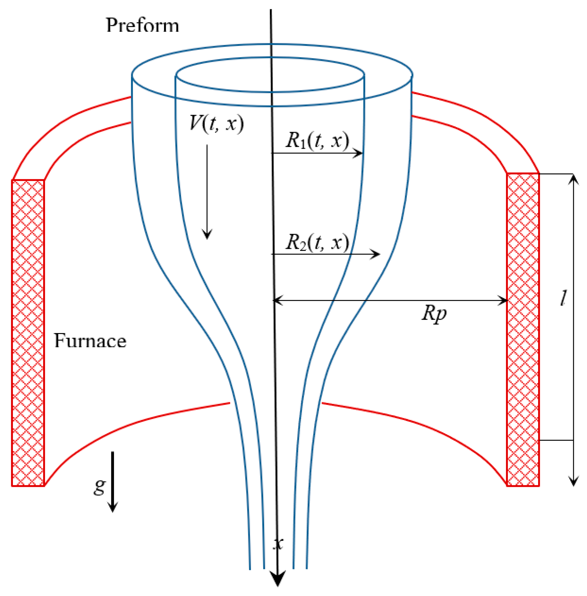
Figure 2.
Radiant heat transfer during capillary drawing.
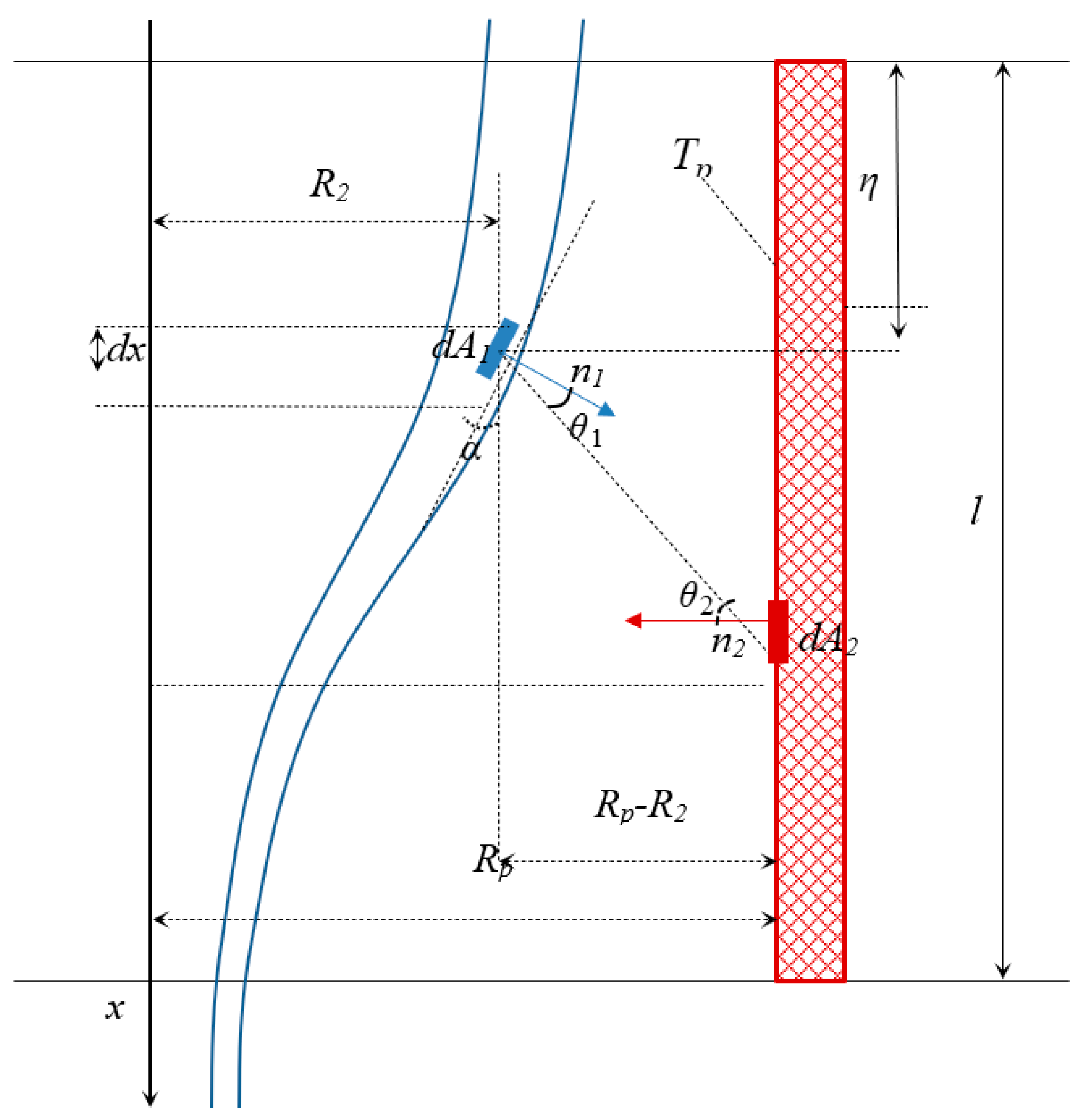
Figure 3.
Dependence of the inner radius of the capillary on the feed and draw rates and the furnace temperature: curves 1, 2 (feed rate 2 × 10⁻³ m/min), curves 3, 4 (feed rate 4 × 10⁻³ m/min), curves 5, 6 (feed rate 8 × 10⁻³ m/min); ▲ (experiment), solid line (calculated values according to the proposed model).

Figure 4.
Examples of typical surface defects in preforms (highlighted in red): (a) air bubbles, (b) streaks, (c) inclusions and contaminations, (d) top material lack.
Figure 4.
Examples of typical surface defects in preforms (highlighted in red): (a) air bubbles, (b) streaks, (c) inclusions and contaminations, (d) top material lack.

Figure 5.
Calculated values of deviations in outer and inner radii in optimal control mode and without it, with optimal control function (in the case of the objective functional (15)): (a) regularization parameter (control cost) ; (b) .
Figure 5.
Calculated values of deviations in outer and inner radii in optimal control mode and without it, with optimal control function (in the case of the objective functional (15)): (a) regularization parameter (control cost) ; (b) .


Figure 6.
Analysis of the values of the regularization parameter (in the case of the objective functional (15)).
Figure 6.
Analysis of the values of the regularization parameter (in the case of the objective functional (15)).
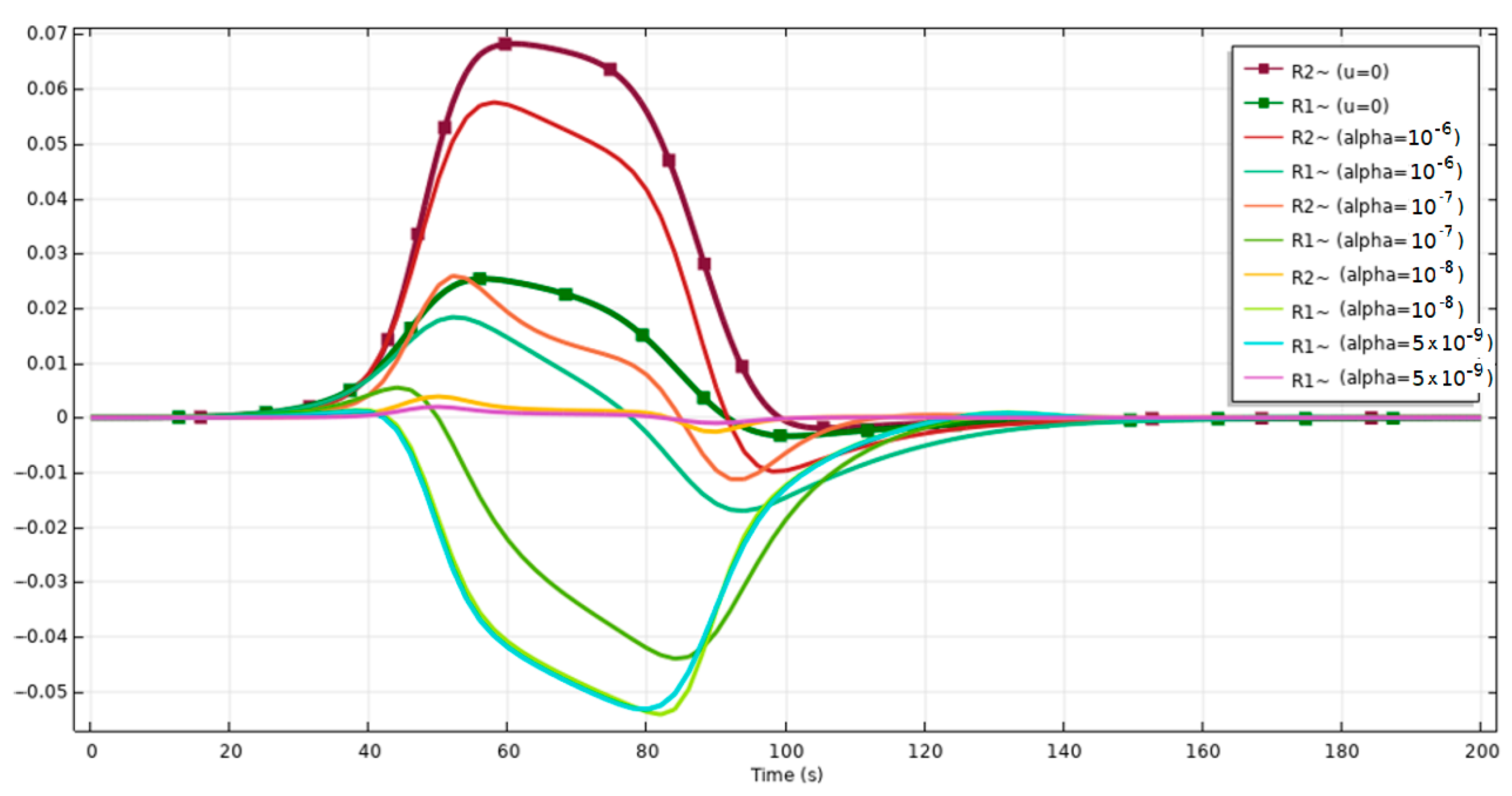
Figure 7.
Geometry of the drawn fiber and optimal control of the capillary drawing speed (in the case of the objective functional (16), ).
Figure 7.
Geometry of the drawn fiber and optimal control of the capillary drawing speed (in the case of the objective functional (16), ).

Figure 8.
Dependence of the component objective functional values (×10−5) on the regularization parameter.
Figure 8.
Dependence of the component objective functional values (×10−5) on the regularization parameter.
Disclaimer/Publisher’s Note: The statements, opinions and data contained in all publications are solely those of the individual author(s) and contributor(s) and not of MDPI and/or the editor(s). MDPI and/or the editor(s) disclaim responsibility for any injury to people or property resulting from any ideas, methods, instructions or products referred to in the content. |
© 2024 by the authors. Licensee MDPI, Basel, Switzerland. This article is an open access article distributed under the terms and conditions of the Creative Commons Attribution (CC BY) license (https://creativecommons.org/licenses/by/4.0/).
Share and Cite
MDPI and ACS Style
Vladimirova, D.; Pervadchuk, V.; Konstantinov, Y. Manufacture of Microstructured Optical Fibers: Problem of Optimal Control of Silica Capillary Drawing Process. Computation 2024, 12, 86. https://doi.org/10.3390/computation12050086
AMA Style
Vladimirova D, Pervadchuk V, Konstantinov Y. Manufacture of Microstructured Optical Fibers: Problem of Optimal Control of Silica Capillary Drawing Process. Computation. 2024; 12(5):86. https://doi.org/10.3390/computation12050086
Chicago/Turabian StyleVladimirova, Daria, Vladimir Pervadchuk, and Yuri Konstantinov. 2024. "Manufacture of Microstructured Optical Fibers: Problem of Optimal Control of Silica Capillary Drawing Process" Computation 12, no. 5: 86. https://doi.org/10.3390/computation12050086
Note that from the first issue of 2016, this journal uses article numbers instead of page numbers. See further details here.