On the Use of Benchmarks for Multiple Properties ^†

Abstract

Benchmark calculations provide a large amount of information that can be very useful in assessing the performance of density functional approximations, and for choosing the one to use. In order to condense the information some indicators are provided. However, these indicators might be insufficient and a more careful analysis is needed, as shown by some examples from an existing data set for cubic crystals.

1. Introduction

An increase in computing power has allowed the replacement of personal experience with databases (see for instance [1,2,3,4,5,6]). In the realm of density functional theory, these have become a valuable tool for both tuning and tailoring new methods (see [7,8,9,10] for recent examples) and, in particular, to assess the performance of density functional approximations [5,11,12]. Ultimately, benchmarks should help computational chemists in choosing the best method to be adopted in a new study. However, the large amount of available data requires synthetic and reliable indicators [13,14,15] capable of providing a ranking based on the quality of the approach. Unfortunately, these indicators do not always give the necessary information, so one has to go back to the database and analyze the data according to the objectives of the study.

Some examples are given below, where indicators might lead to erroneous conclusions:

• choosing the method giving the best results for two properties, A and B;
• choosing the method giving the best results for property B, knowing that property A is well described.

Benchmark calculations for density functionals on some cubic crystals, provided in [16], will be used as a concrete example.

It is not the purpose of this paper to rank density functionals, or to advise for or against any of the density functionals cited here: the questions raised are not connected to any specific functional. Their names appear only in order to facilitate reading and enable reproducibility.

2. When Condensed Information Is Not Sufficient

2.1. Setting the Problem

Consider two methods, X and Y: method X is “better” than method Y for each of the properties A and B taken separately. Should method X be chosen

• when good results are needed for both property A and property B?
• when it is guaranteed (it can be checked) that A is well described, but good results for property B are also needed?

The rapid answer would be to use the method X for both (1) and (2). However, after a brief reflection, it becomes evident that the information provided by the indication that X is better for A and B separately is not sufficient.

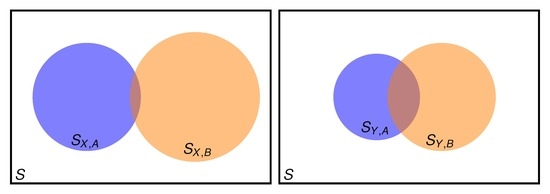
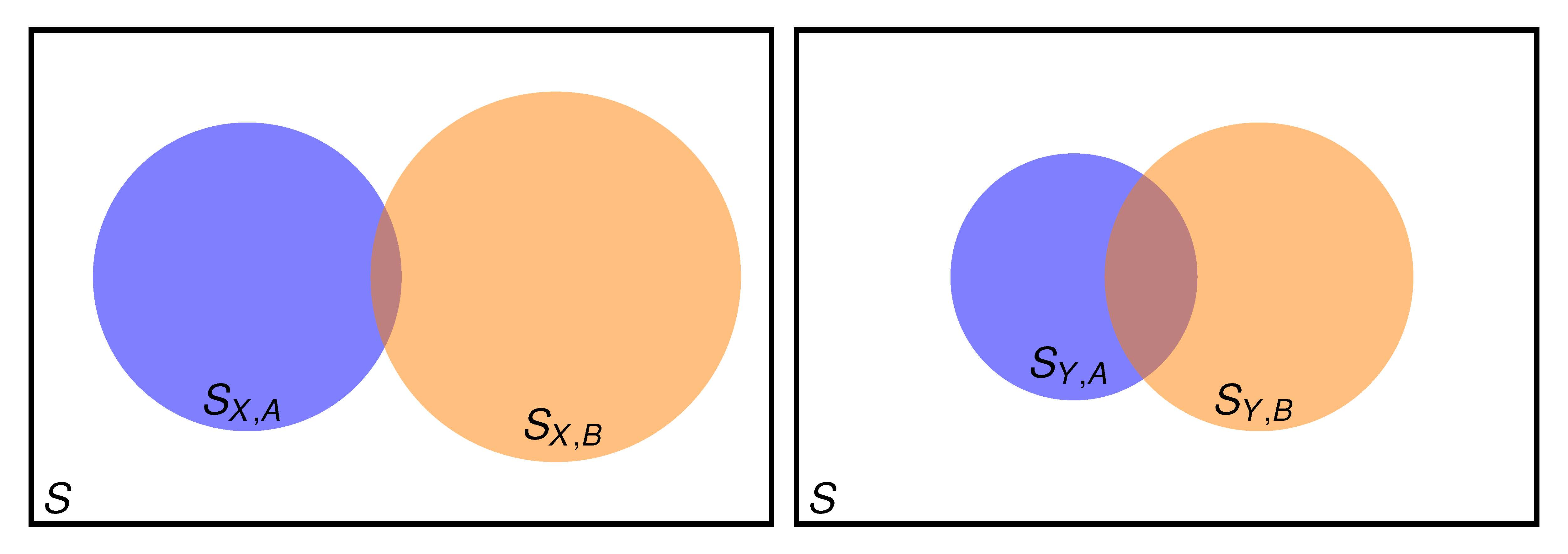
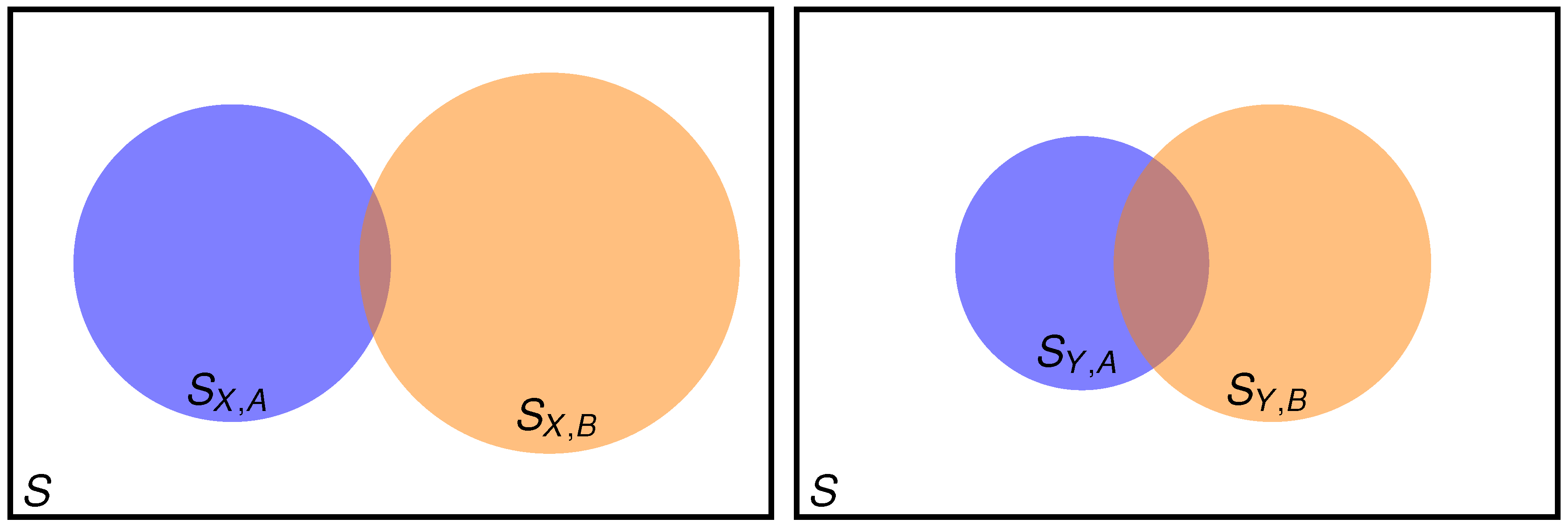
2.2. Two Properties Simultaneously Needed

In order to formalize the problem, let us call the set of systems in the benchmark database, S. The total number of systems is $N\left(S\right)$. A subset $S_{M,P}$ gives “good” results with method $M\in (X,Y)$ for property $P\in (A,B)$. The number of elements in $S_{M,P}$ is $N\left(S_{M,P}\right)$. The probability of obtaining a “good” result with method M for property P is given by $p_{M,P}=N\left(S_{M,P}\right)/N\left(S\right)$. We say that method X is “better” than Y for property P when $N\left(S_{X,P}\right)>N\left(S_{Y,P}\right)$, or $p_{X,P}>p_{Y,P}$.

We now consider the case where $M=X$ is better than $M=Y$ both for $P=A$, and $P=B$. This is schematically represented in Figure 1 by disks corresponding to the subsets $S_{M,P}$. The color of the disks correspond to the properties (blue for property A, orange for property B). The disks in the left panel, corresponding to $M=X$, are larger than in the right panel, corresponding to $M=Y$, indicating that $N\left(S_{X,P}\right)>N\left(S_{Y,P}\right)$. However, we do not have any information about the intersection $S(M,A)\cap S(M,B)$, the number of cases when properties A and B are both well described using method M. We cannot exclude that method X gives “better” results for a larger number of systems $N\left(S_{X,P}\right)>N\left(S_{Y,P}\right)$ and for A and B separately, but that the number of systems for which the results are better both for A and B is smaller for X than for Y: $N(S_{X,A}\cap S_{X,B})<N(S_{Y,A}\cap S_{Y,B})$. A similar result is obtained for the probabilities

$$p_{X,A\cap B}=\frac{N(S_{X,A}\cap S_{X,B})}{N\left(S\right)}<\frac{N(S_{Y,A}\cap S_{Y,B})}{N\left(S\right)}=p_{Y,A\cap B}$$

This is schematically represented in Figure 1 where the overlap of the disks, corresponding to the sets $S_{X,A}\cap S_{X,B}$ (left panel) is smaller than that corresponding to $S_{Y,A}\cap S_{Y,B}$ (right panel). In such a case, when “good” results are desired for both properties, A and B, it is better choose method Y, although method X was better when analyzing each property separately.

To be more specific, let us consider data for cubic crystals given in [16], and choose as A the lattice constants (LC) , and as B the bulk moduli (BM). We consider a method to be “good”, if it reproduces the lattice constants within 3 pm, and bulk moduli within 3 GPa. The probabilities of obtaining “good” results with three different density functional approximations (i.e., LDA [17,18], PBEsol [19] and HISS [20,21]) are given in

Table 1. Probability that a given method gives “good” results for the lattice constants $p_{M,LC}$, for the bulk moduli $p_{M,BM}$, and for both of them $p_{M,LC\cap BM}$. The uncertainty on all reported values, estimated by the Agresti–Coull formula [22], is about $0.1$ for a data set of size 28.

Method	${\mathit{p}}_{\mathit{M}\mathbf{,}\mathit{LC}}$	${\mathit{p}}_{\mathit{M}\mathbf{,}\mathit{BM}}$	${\mathit{p}}_{\mathit{M}\mathbf{,}\mathit{LC}\mathbf{\cap }\mathit{BM}}$	${\mathit{p}}_{\mathit{M}\mathbf{,}\mathit{BM}\mathbf{|}\mathit{LC}}$
LDA	$0.54$	$0.29$	$0.21$	$0.40$
PBEsol	$0.61$	$0.36$	$0.21$	$0.35$
HISS	$0.79$	$0.39$	$0.21$	$0.27$

.

HISS gives the best results both for LC and BM. PBEsol comes next and the local density approximation is the worst. However, when we consider the performance for both LC and BM, LDA, PBEsol, and HISS perform equally. Note that the success probability is rather low.

We would like to stress that the numbers presented in the tables are only to indicate that the effects discussed here can show up. The size of the data set is too small to allow conclusions about the quality of the functionals.

The probability of obtaining a reliable result with method M is not $p_{M,A\cap B}$ as indicated above, but is the probability of obtaining a good result for B given that the result for A is good

$$p_{M,B|A}=\frac{N(S_{M,A}\cap S_{M,B})}{N\left(S_{M,A}\right)}$$

Now the reference set is not the full set of data, S, but the subset of results reliable for A, $S_{M,A}$. Using the same example as above, we find now that $p_{M,BM|LC}$ increases from HISS to PBEsol, and to LDA (Table 1), in reverse order of the probability obtained for $LC$ and $BM$ individually.

Remark 1. 

The problem presented in this paper is related to the lack of positive correlation between the errors made when computing different properties [23]. In the example given in Table 1, the rank correlation coefficients between the errors for lattice constants and bulk moduli are: −0.51 (LDA), −0.24 (PBEsol) and −0.65 (HISS).

3. Improving the Quality of the Approximations Reduces the Risk of Unreliable Selection

The risk of such unpleasant surprises as presented above comes from the low quality of the approximations: in the limiting case when one of the method gives perfect agreement for both properties and the other does not, there is no doubt about which method to choose. In the following we will use a simple approach to improve the performance of the approximations and repeat the analysis made above.

The previous section uses the results directly provided by density functional approximations. A careful analysis of the data reveals that the parametrizations were not good enough to eliminate systematic errors. Having an exact density functional would obviously solve the problems presented above. An efficient way to correct, at least partially, errors of the actual density functionals is to apply a statistical correction, e.g., as a linear transformation [16,24,25]. This correction is a technique to eliminate the main part of the systematic errors, a necessary step to evaluate prediction uncertainty [16].

We now use corrected methods and evaluate their performance on the basis of prediction uncertainty, as reported in [16]. For the same methods as above, one can estimate the success probabilities reported in

Table 2. Probability that a given method gives “good” results for lattice constants $p_{M,LC}$, for bulk moduli $p_{M,BM}$, and for both of them $p_{M,LC\cap BM}$. The uncertainty on all reported values, estimated by the Agresti–Coull formula [22], is about $0.1$ for a data set of size 28. Results are obtained using corrected methods.

Corrected Method	${\mathit{p}}_{\mathit{M}\mathbf{,}\mathit{LC}}$	${\mathit{p}}_{\mathit{M}\mathbf{,}\mathit{BM}}$	${\mathit{p}}_{\mathit{M}\mathbf{,}\mathit{LC}\mathbf{\cap }\mathit{BM}}$	${\mathit{p}}_{\mathit{M}\mathbf{,}\mathit{BM}\mathbf{|}\mathit{LC}}$
LDA	$0.79$	$0.32$	$0.25$	$0.32$
PBEsol	$1.00$	$0.46$	$0.46$	$0.46$
HISS	$0.89$	$0.54$	$0.46$	$0.52$

. One sees that the success probability has notably increased for $LC$ and is slightly less for $BM$. In this group, HISS is not the best method for $LC$ anymore, although it still is for $BM.$

Comparing PBEsol and HISS with LDA individually we notice that the joint and conditional probabilities preserve the supremacy of both “best” methods for individual properties. With PBEsol, as $LC$ is perfect the error only comes from $BM$. Joint and conditional probabilities become equal to $p_{BM}$. With one property perfect, the error of the other determines everything. For HISS, $LC$ is not so good, but $BM$ is better, so the joint probabilities are not worse than for PBEsol and the conditional probabilities are even better than for PBEsol.

4. Conclusions

The wealth of methods available, e.g., density functional approximations, require a selection to be made prior to undertaking a study. This can be made based on benchmark data sets. However, the information condensed from such data sets can be misleading and should be adapted to the study for which the method is chosen.

If a benchmark provides the information that a method X is better than a method Y for some properties $A,B,\dots$ it does not necessarily mean that the method X is better when these properties are all needed for a given study. In other words, the probability of obtaining a “good” result for each of the properties is not the same as the probability of obtaining a “good” result for all the properties. Similarly, when a property can be tested and only systems that pass this test are considered, the statement that a given method is superior to the other methods for each of the properties is insufficient for choosing a functional for the remaining properties. Numerical results from existing benchmarks show that such situations can appear.

The solution to these problems is relatively simple, but one has to go back to the full set of data used in the benchmark and construct the measure relevant to the project. Unfortunately, this is not always possible: benchmarks are not always constructed using the same set of molecules for different properties.

A final remark: although we used “probabilities” to obtain a “good” result in this paper, confusions such as those indicated here can show up also for other measures rating the quality of an approximation.

References

1. Curtiss, L.A.; Raghavachari, K.; Redfern, P.C.; Pople, J.A. Assessment of Gaussian-3 and density functional theories for a larger experimental test set. J. Chem. Phys. 2000, 112, 7374–7383. [Google Scholar] [CrossRef]
2. Curtiss, L.A.; Redfern, P.C.; Raghavachari, K. Assessment of Gaussian-3 and density-functional theories on the G3/05 test set of experimental energies. J. Chem. Phys. 2005, 123. [Google Scholar] [CrossRef]
3. Karton, A.; Daon, S.; Martin, J.M.L. W4-11: A high-confidence benchmark dataset for computational thermochemistry derived from first-principles {W4} Data. Chem. Phys. Lett. 2011, 510, 165–178. [Google Scholar] [CrossRef]
4. Goerigk, L.; Grimme, S. Efficient and accurate double-hybrid-meta-GGA density functionals evaluation with the extended GMTKN30 database for general main group thermochemistry, kinetics, and noncovalent interactions. J. Chem. Theory Comput. 2010, 7, 291–309. [Google Scholar] [CrossRef] [PubMed]
5. Peverati, R.; Truhlar, D.G. Quest for a universal density functional: The accuracy of density functionals across a broad spectrum of databases in chemistry and physics. Philos. Trans. R. Soc. Lond. A 2014, 372. [Google Scholar] [CrossRef] [PubMed]
6. Lejaeghere, K.; Van Speybroeck, V.; Van Oost, G.; Cottenier, S. Error estimates for solid-state density-functional theory predictions: An overview by means of the ground-state elemental crystals. Crit. Rev. Solid State Mater. Sci. 2014, 39, 1–24. [Google Scholar] [CrossRef] [Green Version]
7. Wellendorff, J.; Lundgaard, K.T.; Møgelhøj, A.; Petzold, V.; Landis, D.D.; Nørskov, J.K.; Bligaard, T.; Jacobsen, K.W. Density functionals for surface science: Exchange-correlation model development with Bayesian error estimation. Phys. Rev. B 2012, 85. [Google Scholar] [CrossRef]
8. Wellendorff, J.; Lundgaard, K.T.; Jacobsen, K.W.; Bligaard, T. mBEEF: An accurate semi-local Bayesian error estimation density functional. J. Chem. Phys. 2014, 140. [Google Scholar] [CrossRef] [PubMed] [Green Version]
9. Mardirossian, N.; Head-Gordon, M. xB97X-V: A 10-parameter, range-separated hybrid, generalized gradient approximation density functional with nonlocal correlation, designed by a survival-of-the-fittest strategy. Phys. Chem. Chem. Phys. 2014, 16, 9904–9924. [Google Scholar]
10. Yu, H.S.; Zhang, W.; Verma, P.; Xiao Heac, X.; Truhlar, D.G. Nonseparable exchange–correlation functional for molecules, including homogeneous catalysis involving transition metals. Phys. Chem. Chem. Phys. 2015, 17, 12146–12160. [Google Scholar] [CrossRef] [PubMed]
11. Goerigk, L.; Grimme, S. A thorough benchmark of density functional methods for general main group thermochemistry, kinetics, and noncovalent interactions. Phys. Chem. Chem. Phys. 2011, 13, 6670–6688. [Google Scholar] [CrossRef] [PubMed]
12. Hao, P.; Sun, J.; Xiao, B.; Ruzsinszky, A.; Csonka, G.I.; Tao, J.; Glindmeyer, S.; Perdew, J.P. Performance of meta-GGA functionals on general main group thermochemistry, kinetics, and noncovalent interactions. J. Chem. Theory Comput. 2013, 9, 355–363. [Google Scholar] [CrossRef] [PubMed]
13. Civalleri, B.; Presti, D.; Dovesi, R.; Savin, A. On choosing the best density functional approximation. In Chemical Modelling: Applications and Theory; Royal Society of Chemistry: London, UK, 2012; Volume 9, pp. 168–185. [Google Scholar]
14. Savin, A.; Johnson, E.R. Judging density functional approximations: Some pitfalls of statistics. Top. Curr. Chem. 2015, 365, 81–95. [Google Scholar]
15. Perdew, J.P.; Sun, J.; Garza, A.J.; Scuseria, G. Intensive atomization energy: Re-thinking a metric for electronic-structure-theory methods. Z. Phys. Chem. 2016, in press. [Google Scholar] [CrossRef]
16. Pernot, P.; Civalleri, B.; Presti, D.; Savin, A. Prediction uncertainty of density functional approximations for properties of crystals with cubic symmetry. J. Phys. Chem. A 2015, 119, 5288–5304. [Google Scholar] [CrossRef] [PubMed]
17. Slater, J.C. A simplification of the hartree-fock method. Phys. Rev. 1951, 81, 385–390. [Google Scholar] [CrossRef]
18. Vosko, S.H.; Wilk, L.; Nusair, M. Accurate spin-dependent electron liquid correlation energies for local spin density calculations: A critical analysis. Can. J. Phys. 1980, 58, 1200–1211. [Google Scholar] [CrossRef]
19. Perdew, J.P.; Ruzsinszky, A.; Csonka, G.I.; Vydrov, O.A.; Scuseria, G.E.; Constantin, L.A.; Zhou, X.; Burke, K. Restoring the density-gradient expansion for exchange in solids and surfaces. Phys. Rev. Lett. 2008, 100. [Google Scholar] [CrossRef] [PubMed]
20. Henderson, T.M.; Izmaylov, A.F.; Scuseria, G.E.; Savin, A. The importance of middle-range hartree-fock-type exchange for hybrid density functionals. J. Chem. Phys. 2007, 127. [Google Scholar] [CrossRef] [PubMed]
21. Henderson, T.M.; Izmaylov, A.F.; Scuseria, G.E.; Savin, A. Assessment of a middle-range hybrid functional. J. Chem. Theory Comput. 2008, 4, 1254–1262. [Google Scholar] [CrossRef] [PubMed]
22. Brown, L.D.; Cai, T.T.; DasGupta, A. Interval estimation for a binomial proportion. Stat. Sci. 2001, 16, 101–133. [Google Scholar]
23. Lejaeghere, K.; Vanduyfhuys, L.; Verstraelen, T.; Speybroeck, V.V.; Cottenier, S. Is the error on first-principles volume predictions absolute or relative? Comput. Mater. Sci. 2016, 117, 390–396. [Google Scholar] [CrossRef]
24. Duan, X.M.; Song, G.L.; Li, Z.H.; Wang, X.J.; Chen, G.H.; Fan, K.N. Accurate prediction of heat of formation by combining Hartree-Fock/density functional theory calculation with linear regression correction approach. J. Chem. Phys. 2004, 121. [Google Scholar] [CrossRef] [PubMed] [Green Version]
25. Lejaeghere, K.; Jaeken, J.; Speybroeck, V.V.; Cottenier, S. Ab initio based thermal property predictions at a low cost: An error analysis. Phys. Rev. B 2014, 89. [Google Scholar] [CrossRef]
Figure 1. Diagrammatic explanation that method X can be better than method Y for property A and property B when taken separately, but method Y is better when both A and B are needed. Blue disks: cases when the method works well for property A; orange disks: cases when the method works well for property B; (left) method X; (right) method Y.
Computation 04 00020 g001